Bayesian variable selection for parametric survival model with applications to cancer omics data

P R I M A R Y R E S E A R C H

Open Access

Bayesian variable selection for parametric

survival model with applications to cancer

omics data

Weiwei Duan

, Ruyang Zhang

, Yang Zhao

, Sipeng Shen

, Yongyue Wei

,

Feng Chen

and David C. Christiani

Abstract

Background:Modeling thousands of markers simultaneously has been of great interest in testing association between genetic biomarkers and disease or disease-related quantitative traits. Recently, an expectation-maximization (EM) approach to Bayesian variable selection (EMVS) facilitating the Bayesian computation was developed for continuous or binary outcome using a fast EM algorithm. However, it is not suitable to the analyses of time-to-event outcome in many public databases such as The Cancer Genome Atlas (TCGA).

Results:We extended the EMVS to high-dimensional parametric survival regression framework (SurvEMVS). A variant of cyclic coordinate descent (CCD) algorithm was used for efficient iteration in M-step, and the extended Bayesian information criteria (EBIC) was employed to make choice on hyperparameter tuning. We evaluated the performance of SurvEMVS using numeric simulations and illustrated the effectiveness on two real datasets. The results of numerical simulations and two real data analyses show the well performance of SurvEMVS in aspects of accuracy and computation. Some potential markers associated with survival of lung or stomach cancer were identified.

Conclusions:These results suggest that our model is effective and can cope with high-dimensional omics data.

Keywords:Survival analysis, Bayesian variable selection, EM algorithm, Omics, Non-small cell lung cancer, Stomach adenocarcinoma

Introduction

With the development of high-throughput sequence tech-nology, large-scale omics data are generated rapidly for discovering new biomarkers [1, 2]. The public databases such as The Cancer Genome Atlas (TCGA) and Gene Expression Omnibus (GEO) provide great opportunities to understand complex diseases comprehensively on a molecular level [3,4] and subsequently facilitate growing demanding statistical approaches designed to cope with these large-scale data [5]. Analyzing biomarkers one at a time is the most common strategy to detect the

underlying causal markers [6, 7]. However, this

one-by-one method ignores the correlation between bio-markers and needs multiple corrections for controlling false positives. Furthermore, multiple regression is per-formed increasingly because it is powerful to identify causal markers after the strongest associations have been accounted for [8–10]. It can also avoid multiple correction and enable accurate effect estimation [11, 12]. Neverthe-less, omics data generally have the property of high

di-mensionality, which makes the classical multiple

regression yield unstable parameter estimations with high standard errors. Due to this limitation, least absolute shrinkage and selection operator (LASSO) regression and its variants shrink the effects of noise toward zero while adding a penalty term to the likelihood function. The ap-proach can easily be conducted on a large-scale variable selection analysis [13, 14]. The LASSO can also be ex-plained from Bayesian perspectives, namely Bayesian * Correspondence:[email protected]

†_{Weiwei Duan and Ruyang Zhang contributed equally to this work.}

1_{Department of Biostatistics, School of Public Health, Nanjing Medical}

University, 101 Longmian Avenue, Nanjing 211166, Jiangsu, China

2_{China International Cooperation Center for Environment and Human Health,}

Nanjing Medical University, 101 Longmian Avenue, Nanjing 211166, Jiangsu, China

Full list of author information is available at the end of the article

© The Author(s). 2018Open AccessThis article is distributed under the terms of the Creative Commons Attribution 4.0

International License (http://creativecommons.org/licenses/by/4.0/), which permits unrestricted use, distribution, and

LASSO (BL) [15]. That is, we can generate the LASSO es-timators by imposing a Laplace prior on coefficients of ex-planatory variables. Compared with a frequentist penalty, Bayesian regression is more flexible to induce different shrinkage by specifying various priors.

George and McCulloch [16] proposed a two-component

“spike-and-slab”mixture prior, consisting of the“spike” to

be either a point mass at zero or a normal distribution with a very narrow variance while a“slab”be a normal distribu-tion with a large variance. Indicator variables are utilized to denote which component each marker belongs to, which is known as Bayesian variable selection (BVS). BVS and its ex-pansions are widely used in genomic studies, including marker detection and disease risk prediction [11, 12, 17]. But, most Bayesian studies have used a Markov Chain Monte Carlo (MCMC) algorithm to explore the posterior distribution of unknown parameters via numerical approxi-mations in high-dimensional models, which is quite time consuming for getting a stable chain. For example, the BayesR model required ~ 18 h to complete an analysis of a bipolar disorder genome-wide association data with ~ 3800 individuals (80% of whole samples) and ~ 300,000 genotype markers [12]. In order to facilitate Bayesian computation, variational inference [18–20] and expectation-maximization (EM) algorithm are commonly used for Bayesian posterior inference [21]. Ročková and George [22] proposed EM vari-able selection (EMVS) for continuous outcomes to rapidly identify promising high posterior models and parameter esti-mates. The continuous conjugate spike-and-slab prior adopted by EMVS leads to fast closed form expression for the EM algorithm. Nevertheless, there has been considerable interest in discovering associations between biomarkers and prognosis.

Analyzing time-to-event data, namely survival analysis, plays a very important role in statistics, which arises in many fields, such as medicine, genetics, industrial engin-eering, sociology, and economics [23–25]. Modeling sur-vival data using Cox proportional hazards regression is popular for its robust to the unknown baseline hazard [26]. Alternatively, being well known for parametric sur-vival analysis, accelerated failure time (AFT) model tends to give more precise estimates of interest parame-ters if the distribution of survival time is chosen cor-rectly, in addition, the parameter estimates from AFT are robust to omitted covariates [27]. Under the scenario of high-dimensional survival analysis, a lot of works have been done usually by adding a penalty term to likeli-hood. In a Bayesian framework, we usually need to as-sign a semi-parametric or nonparametric prior processes to the (cumulative) baseline hazard function in a Cox

model [28, 29], which does not allow us to naturally

choose a fully parametric survival model for the subse-quent analyses. As a parametric model, the Weibull re-gression induces a very flexible model since it is a

unique parametric model which has both AFT and the proportional hazards properties [30].

In this study, we extended EMVS to parametric sur-vival model (SurvEMVS) with Weibull distribution as-sumption. A fast EM algorithm was used to obtain posterior modes of interested parameters, in which a variant of the fast cyclic coordinate descent (CCD) method is nested. We used simulation trials to explore performance in comparison with an alternative frequen-tist variable selection strategy, namely Cox LASSO re-gression. After that, we applied SurvEMVS to a lung cancer genotype data and a stomach cancer gene expres-sion data. Further details of this work were given below.

Methods

Statistical framework

Survival times ofnindividuals in sample are designed by

Ti= min(ti,ci),i= 1,…,n, wheretiandciare lifetime and

fixed censoring time for a specific individual i, respect-ively. The survival outcome from a follow-up study can be conveniently represented by pair of random variables (Ti,

δi), whereδiindicates whether the lifetimeticorresponds

to an event (δi= 1) or is censored (δi= 0). In this study, we

consider right censoring scheme and non-informative censoring mechanism for each individual without note elsewhere. Under parametric framework,f(Ti|θ) andS(Ti|

θ) are defined as probability density and survival function of survival timeTi, respectively, parametrized byθ. Let L

¼Qn

i¼1fðTijθÞδiSðTijθÞð1−δiÞbe the likelihood of the

para-metric model with an i.i.d assumption. Weibull

distribu-tion can be fully parametrized by the parameter pair θ

= (λ,α), whereλandαare scale and shape parameter, re-spectively. The density and survival function of Weibull distribution Tare f(T|λ,α) =αTα−1λexp(−λTα) and S(T|

λ,α) = exp(−λTα), respectively. Typically in a regression model, the scale parameter is defined as λ= 1/ exp(Zu+

Xβ), where Xn×p represents a column-scaled matrix of

tumor biomarkers such as gene expression, genotype or

DNA methylation, β is a p× 1vector of marker effects,

Zn× (1 +q)is a covariates matrix of intercept and q clinical

variables such as gender, age, and tumor histological grade,uis a (q+ 1)-dimensional effect vector ofZn× (1 +q).

With the condition of p>n(i.e., high dimension), a penalize term is necessary for inducing a sparse solution ofβ. Under the Bayesian framework, we want to impose a well-known spike-and-slab prior on each βj to facilitate

Bayesian variable selection [16]. A vector of binary latent variablesγ= (γ1,…,γp)T, γj∈{0, 1} are introduced as

indi-cator variables, where γj= 1 donates that jth explanatory

variable is to be included in the model. Conditional onγ, the continuous prior being assigned toβis,

πβjσ2_;γ¼N

p 0;Dσ2_;γ

where Dσ2_;γ ¼σ2 diagða1;…;apÞand a_j= (1−γ_j)υ₀+γ_jυ₁. As suggested by [22], we set these hyperparameters υ0 andυ1to be small and large positive values, respectively.

σ2

is a common variance parameter with an inverse gamma prior π(σ2) =IG(ν/2,νη/2). The binomial prior is chosen for the indicator variable γ, i.e., πðγjθÞ ¼Qp_j¼1

θγjð₁−θÞ1−γj_{, where} θ _{is a hyperparameter and we} im-pose a Beta(a, b) prior on it. The constant prior is chosen forαandu, i.e.,π(α)∝1 andπ(u)∝1.

Generally speaking, MCMC is usually used for simu-lating the posterior distribution of unknown parameters

β, γ, θ, σ2, α, and u. But here we employ an EM algo-rithm to seek the posterior mode of each parameter be-cause this algorithm provides substantial computational advantage, especially for high-dimensional data analysis.

Concerning about the unknown status γ for variables,

we replace this “missing data”by its conditional expect-ation given the current estimates for other parameters

and observed data (E-step) [31]. Then, an M-step is

followed by maximizing the expected complete-data log-posterior with respect to β, θ, σ2, α, and u. As a re-sult of iterations between the E-step and M-step, each estimator will converge toward a local maximum of the posterior distribution. More specifically, the objective function can be expressed as:

Qðβ;θ;σ2;α;ujT;δÞ ¼Eγj½logπðβ;γ;θ;σ2;α;ujT;δÞ

¼CþlogLþEγj½logπðβjσ2;γÞ

þEγj½logπðγjθÞ;

þlogπðθÞ þlogπðσ2Þ þlogπðαÞ þlogπðuÞ

ð2Þ

where E_{γ∣ ⋅}(⋅) denotes the expectation with regard

to γ given estimations in current iteration.

Further-more, Eγj½logπðβjσ2;γÞ ¼C1−p₂ logσ2−₂1_σ2

Pp j¼1β2jEγj

½ð1−γjÞυ0þγjυ1

−1

, and Eγj½logπðγjθÞ ¼Ppj¼1Eγj½γj

logð₁θ_−θÞ þplogð1−θÞ, both C and C1 are constants. Next, our EM algorithm for Bayesian Weibull regres-sion proceeds as follows.

(1) Initialize the unknown parameters:β(0),θ(0),σ2(0),

α(0)

,u(0). (2) E-step:

As can be seen from the formula (2) above, there are two parts that need further evaluation, namely Eγ∣ ⋅[γj]

and Eγ∣ ⋅[(1−γj)υ0+γjυ1]−

1

. In particular, Eγ∣ ⋅[γj] is a

conditional expectation of γj and depends on observed

data (T,δ) only by means of current parameter estimates

β(k)

,θ(k), σ2(k)because of the hierarchical structure of γ; therefore, we have

Eγj γj

h i

¼P γ_j¼1jβð Þk;θð Þk;σ2ð Þk

¼p_j; ð3Þ

where p_j ¼ πðβ

ðkÞ

j jσ2ðkÞ;γj¼1ÞPðγj¼1jθð kÞ_Þ

πðβðkÞ

j jσ2ðkÞ;γj¼1ÞPðγj¼1jθð kÞ_ÞþπðβðkÞ

j jσ2ðkÞ;γj¼0ÞPðγj¼0jθð kÞ_Þ ;

meanwhile, the second part will be easily derived as

Eγj 1−γj

υ0þγjυ1

h i−1

¼1−pj

υ0 þ

p_j υ1¼

d_j: ð4Þ

(3) M-step:

Next, we derive the M-step for the objective function

Q(β,θ,σ2,α,u|T,δ).

1) DifferentiatingQ(⋅|T,δ) with regard toβneeds to solve the following expression

βðkþ1Þ_{¼ arg min}

β −logLþ 1 2σ2 D

1=2_β

2

; ð5Þ

2) DifferentiatingQ(⋅|T,δ) with regard touj,j= 1,…, q+ 1one-by-one using one-dimensional

optimization reveals the following form

uð_jkþ1Þ _βðkþ1Þ_;α;σ2_;θ;uðkþ1Þ j− ;ujþ

¼uj−∂

logL

∂uj

∂2_logL ∂u2

j

!−1

;

ð6Þ

with all other parameters being fixed at current estimates.

3) DifferentiatingQ(⋅|T,δ) with regard toαderives the following form

αðkþ1Þ

βðkþ1Þ_;uðkþ1Þ_;σ2_;θ

_¼α−∂logL

∂α

∂2 _logL ∂α2

−1

: ð7Þ

4) Forσ2, we have

σ2ðkþ1Þ_¼

Pp

j¼1β kþ1

ð Þ2 j djþνη

pþνþ2 : ð8Þ

5) Forθ, we have

θðkþ1Þ_¼

Pp

jpjþa−1

aþbþp−2: ð9Þ

(4) Iterations between the E-step and M-step are in progress. SurvEMVS will be terminated if the con-vergence criterion is satisfied as follows:Pn_i¼1jXT

i ð

βðkÞ_−βðk−1Þ_Þj=ð1þPn

i¼1jXTiβðkÞjÞ<ξ, whereXβ

(k)

is predictive vector atkth iteration, andξis a small value (say 10−4). Summarizing, Additional file1: Figure S1 presents pseudocode for our implementa-tion of SurvEMVS.

Simulation studies

In this section, we used simulations to validate the per-formance of proposed SurvEMVS. Cox LASSO model

[35] was considered as a benchmark for comparison.

The effect sizes and directions of Cox LASSO estimates

were adjusted for consistency with our parametric model, which made the direct comparison between two methods. For each simulation scenario, we replicated the simulation 50 times and then summarized these results.

Marker values were simulated from a multivariate nor-mal distribution N50(0,∑), where∑is a variance-covariance symmetric matrix with ∑jj= 1 and ∑ij= 0.6|i−j|, i≠j. For

largepmarkers, we repeatedly sampled from the above dis-tribution and then combined them by column. Thus, we obtained ann×pmatrix with multiple independent blocks and 50 makers in each block were correlated. Assuming

λi¼ expð−

Pp

jxijβjÞ, we simulated survival time ti for

each subject from an exponential distributionti

~exponen-tial(λi) , and random censoring timecifrom a uniform

dis-tribution ci~U(0, K), and chose K such that on average

40% subjects were right censored. The observed censored survival timeTiwas generated by min(ti,ci). Furthermore,

additional simulations where survival times are generated from Weibull distribution (withα= 2) were used to show effectiveness of our method. As is well-known, the true distribution of survival time in a real data is unclear and does not coincide with the Weibull assumption exactly. Therefore, we simulated a vector of Gamma-distributed survival time on purpose, thus assigning weakness setting to SurvEMVS. The shape and rate parameters of gamma distribution were set to be 0.8 and 1/λi, respectively. We

randomly sampled six causal markers and set coefficients

to be {0.2, −0.2, 0.3, −0.3, 0.4, −0.4}. Sample size

(n) was set to be 500, and number of makers is set to be 1000 or 5000. Moreover, we generated 100 samples as a test dataset in each replication to appreciate the predictive performance of two approaches. The detailed simulation scenarios were summarized in Table1.

Hyperparameters tuning and performance metric

The performance of SurvEMVS depended on the hyper-parametersυ0andυ1, which made us be interested in a run-ning model based on more than one combination ofυ0and

υ1. The speed of the EM algorithm made it feasible to con-sider a sequence of models as (υ0,υ1) varied over many

can-didates, from which we could select an optimal

combination based on some criteria. According to [22], largeυ1and smallυ0could accommodate all plausibleβj. In

order to acquire sparse solution in largepdata, we set a se-quence of candidates {1/10p, 1/5p, 1/2p, 1/p, 2/p, 5/p, 10/p, 0.05} (0.05 was reserved if p> 500) to υ0unless otherwise

noted, which was dynamic with p. Three candidates from

{10, 100, 500} were assigned toυ1. Therefore, there were 24 combinations for hyperparameter tuning. The procedure

of fitting Cox LASSO by widely used R package glmnet

gave the similar parameter tuning as we did here.

On account of making parameter selection from the

measure the performance of the fitted models. Cross-validation partial likelihood (CVPL) was generally

used for parameter selection in Cox model [35, 36],

while some employed cross-validation score in paramet-ric survival model [36]. Subsequently, one candidate of hyperparameters was chosen to minimize one of these metrics. However, these metrics involving random cross-validation (CV) make the hyperparameter selec-tion not stable as well as time demanding, and depend on the folds. Other criteria without CV like the Akaike information criterion (AIC), the Bayesian information criterion (BIC), and the generalized cross-validation (GCV) tend to select many spurious variables especially in high-dimensional problem [37, 38]. In this paper, we considered a metric, namely extended Bayesian Informa-tion Criteria (EBIC), which was utilized for model

selec-tion at first [39]. The constant prior behind the BIC

assigns high probabilities to the models with a larger number of markers, which was apparently unreasonable and strongly against the principle of parsimony. The EBIC was proposed to take away this disadvantage of the BIC. The EBIC is defined as,

EBICγ ¼−2 logLþpm logn

þ2τ p

p_m

;0≤τ≤1; ð10Þ

where pm is the number of selected variables in a fitted model. The EBIC withτ= 0 reduces to the original BIC. Minimizing the EBIC with largerτwill get a much more parsimonious model. Thus, EBIC1, EBIC2, and EBIC3 were served as metrics for hyperparameter tuning with regard toτ= 0, 0.5, 1, respectively.

In simulation studies, the optimal SurvEMVS model selected by the EBIC was compared with Cox LASSO in aspects with variable selection, effect estimation, and model prediction. We utilized false positive rate (FPR), true positive rate (TPR), and false discovery rate (FDR) as evaluation indicators for variable selection. Note that

Pðγ_j¼1j^β_j;^θ;σ^2Þ≥0:5 meant the jth maker was

se-lected. Mean square error (MSE) denoted by Pp_j¼1

ð^βj−βjÞ

2

=p was used to appreciate effect estimations for makers. The predictive accuracy of the fitted model be applied to test dataset was evaluated by Harrell’sc

statis-tic [40], as known as the area under the ROC curve

(AUC).

Implementation

We considereda=b= 1 in beta prior forθwhich yielded a uniform distribution. As noted in [22], we had inverse

gamma prior for σ2 with ν=η= 1 to make this prior

relatively non-influential. We ran all analyses using R software (v3.41) on a machine with Intel® Xeon® X5690 3.46-GHz processors. Cox LASSO model was

imple-mented with the glmnet package in R. Tenfold

cross-validation was used to choose an optimal penaliza-tion parameterλlassoinglmnet, which determined an

op-timal Cox LASSO model. Two LASSO models selected

by“minimum cvm”and “1 standard error” ofλlassowere

considered as LASSO.min and LASSO.se, respectively. We employed the PLINK tool for quality control of genotype data [41].

Results

Simulation studies

Iteration and tuning plot

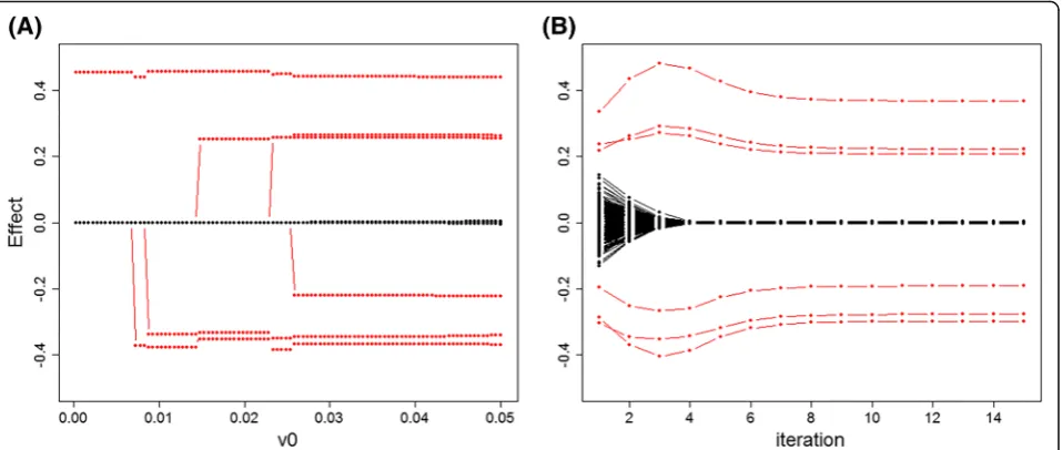
By analogy with LASSO solution path plot that shows the estimates change with an increasing penalty param-eter, here we want to investigate the impact of parame-ters tuning for υ0. Figure 1a displays a solution path of

SurvEMVS under Scenario 1 with υ1=10. Large effects

(red dots) will be firstly incorporated into the fitting

model with υ0 increasing, and a remarkable separation

between the positive and negative effects appears when

υ0is larger than 0.03. However, the estimated effects for zeros inflate because of less shrinkage at large υ0. We also present the iteration plot to detect the convergence

property of our approach. From Fig. 1b, SurvEMVS

makes a fast convergence to posterior estimates only in several steps. Moreover, neutral effects (black dot line) get close to zero in the fourth iteration, which means that we can concentrate iterations on large effects after a

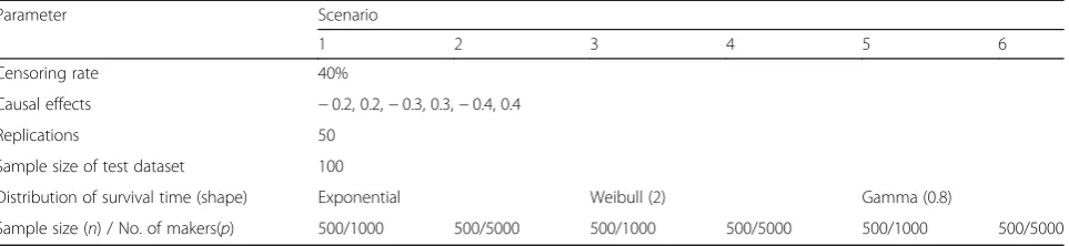
Table 1Parameters settings for simulation studies

Parameter Scenario

1 2 3 4 5 6

Censoring rate 40%

Causal effects −0.2, 0.2,−0.3, 0.3,−0.4, 0.4

Replications 50

Sample size of test dataset 100

Distribution of survival time (shape) Exponential Weibull (2) Gamma (0.8)

number of full iterations for all makers and further ac-celerate the posterior computation.

Variable selection

In SurvEMVS, conditional posterior probabilities are used to guide variable selection. Table2shows compari-son results between SurvEMVS and Cox LASSO in vari-able selection for Scenarios 1 and 2. For Scenario 1 with

p= 1,000, all models except LASSO.min can reduce

noise markers with low FDRs, and all of three models with regard to SurvEMVS acquire high TPRs. When

simulated p increases to 5000 (Scenario 2), FPR and

FDR of BIC (i.e., EBIC1) inflate seriously. These indicate that proper extra penalty on the BIC of SurvEMVS brings to a moderate result of variable selection. We summarize the results of Scenarios 3 and 4 with Weibull distribution in Additional file1: Table S1, and the results of Scenarios 5 and 6 with gamma distribution in Add-itional file 1: Table S2. Each of them presents a similar trend with scenarios of exponential distribution.

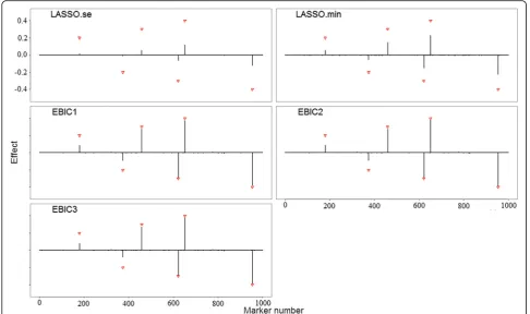
Parametric estimation

Figure2and Additional file1: Figures S2-S6 show the par-ameter estimations of five models for all scenarios. Aver-aged estimated effects (black vertical lines) of estimated effects for all makers are calculated over 50 trials. Trian-gles in all figures label the locations and effect sizes of the pre-specified causal makers. In all scenarios, SurvEMVS gives a lower bias than Cox LASSO. Biases of all models increase with number of variants. Two models of Sur-vEMVS (i.e., EBIC2 and EBIC3) present a similar estima-tor, while the estimated effects in EBIC1 for zeros inflate

under scenarios with p= 5,000 (rough X-axis in

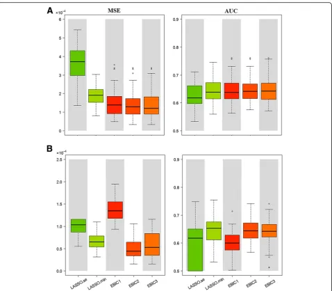
Add-itional file1: Figures S2, S4 and S6). In order to make a comprehensive evaluation of bias and variance, we use the MSE metric and present the results in the left panels of Fig. 3 and Additional file 1: Figures S7 and S8. Both the EBIC2 and EBIC3 are well performed under all scenarios,

whereas the EBIC1 model get a high MSE withp= 5,000.

There is no apparent difference between the results of ex-ponential, Weibull, and gamma distribution.

Prediction accuracy

In order to appreciate prediction accuracy of the fitted models, we summarize AUC results by box plot in the right panels of Fig.3and Additional file1: Figures S7 and S8. Generally speaking, the EBIC2 model performs best under our simulation settings, while the LASSO.min pre-sents similar prediction but with larger variance. In ac-cordance with the conclusion of “Parametric estimation”,

prediction accuracy of the BIC model descends with p

varying from 1000 to 5000. Moreover, SurvEMVS with ex-ponential or Weibull settings gain slightly larger AUC than those with the gamma settings. Furthermore, the Fig. 1Solution path and iteration path of the proposed SurvEMVS under Scenario 1. Red dots represent the changes of estimated effects for the

true signals.aSolution path.bIteration path (υ0= 0.05)

Table 2TPR, FPR, and FDR in variable selection with 50 replications (exponential distribution)

Method Scenario 1 (p= 1000) Scenario 2 (p= 5000)

TPR FPR FDR TPR FPR FDR

LASSO.se 0.657 1.25E−03 0.239 0.327 1.36E−04 0.258

LASSO.min 0.920 2.11E−02 0.792 0.713 4.60E−03 0.843

EBIC (τ= 0) 0.743 1.19E−03 0.209 0.703 5.78E−03 0.872

EBIC (τ= 0.5) 0.730 7.85E−04 0.151 0.480 1.48E−04 0.204

EBIC (τ= 1.0) 0.710 6.24E−04 0.127 0.377 2.00E−05 0.042

LASSO.se model almost provides the lowest AUC among simulation scenarios. All the above results indicate that the BIC is not suitable for largepscenario.

In summary, the EBIC2 model works best under almost all scenarios in terms of variable selection, parameter esti-mation, and prediction accuracy. Besides, Additional file1: Table S3 shows the time consumption in different scenar-ios. In comparison with Cox LASSO, SurvEMVS takes more computational time but is still fast enough. Note that time used in Additional file1: Table S3 is for refer-ence only, as it varies depending on context, such as con-vergence criterion, programming language, computer performance, and algorithm optimization.

Real data analysis

Harvard lung cancer data

This dataset from The Harvard Lung Cancer Susceptibility Study GWAS includes 526 late-stage (III and IV) patients with non-small cell lung cancer (NSCLC) recruited from Massachusetts General Hospital (Boston, MA). More de-tails about participants’ recruitment have been described previously [42]. We note that it is appropriate to assess an association study restricted to late-stage cancer because some gene functions work primarily in the late stage and are not present in preinvasive stages of cancer [43]. DNA was genotyped using Illumina 610K Quad chip. After

quality control protocol described by [44], there were 512,885 SNPs remaining. Those patients with more than 5 years of overall survival were considered as right cen-sored, and finally, the censor rate was equal to 20.27%. We assumed an additive genetic model and imputed missing genotypes by mean of each SNP. We adjusted for age, sex, smoking status, cell type, stage, surgery (yes vs. no), and the top four principal components in the subsequent analysis. Considering that the number of SNPs related to NSCLC survival was not expected to be too large, we filtered the SNPs by a commonly used single locus Cox model. This fil-ter yielded a de-noising of outcome so that the subsequent analyses became more efficient. By setting a threshold ofP

value less than 5E−3, 3911 SNPs were left for the subse-quent analysis.

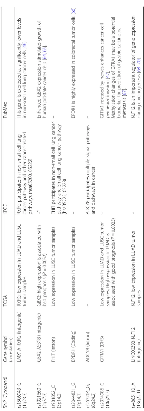
The EBIC2 was used to choose an optimal model from the candidates we noted above. Finally, 14 SNPs were detected

by the proposed EBIC2 model with υ1= 100 and

υ0=2.56E-03. We further analyzed and annotated these SNPs

by TCGA (with an online tool UALCAN [45]), KEGG

and TCGA-LUSC (lung squamous cell carcinoma) tumor samples and samples of other research [46]. Additionally, it also participates in non-small cell lung cancer path-ways and other cancer-related pathpath-ways. rs2074986 is located at DNase I hypersensitive site (DHS) of GFRA1 on Chromosome 10. GFRA1 released by

nerves enhances cancer cell perineural invasion [47],

whose expression is reduced in tumor samples of TCGA-LUAD and TCGA-LUSC compared with nor-mal samples. In addition, the high expression level in TCGA-LUAD tumor samples may contribute to good

prognosis (P= 0.0025). We also provided the

esti-mated effects of 14 SNPs by SurvEMVS in

Add-itional file 1: Table S4 along with classical Weibull

regression estimations for them (that is, only 14 SNPs and clinical variables are fitted by Weibull regression). In this way, SurvEMVS applied in high-dimensional

data can also generate approximate estimates with Weibull regression. We plotted Kaplan-Meier (KM) survival curve of patients with high, moderate, and low risk defined by tertiles of risk scores −Pp_jxijβj

(Additional file1: Figure S9). The log-rank test was used to compare the survival estimates among the three groups, and the results show that higher prognostic risk score is significantly associated with shorter survival (P< 1E−16). However, Cox LASSO models did not identify any SNP.

TCGA stomach adenocarcinoma (TCGA-STAD) expression data

We accessed this RNA-seq transcriptomic data from

TCGA database by R/Bioconductor package

TCGAbio-links[48], which was used to do subsequent quality

con-trol, normalization, differential expression analysis

(DEA), and visualization. The clinical information is summarized in Additional file1: Table S5. Similar to the first real data analysis, we built final models only using filtered expression markers by DEA rather than all markers. There were 2711 markers left passing a selec-tion threshold defined at fold change (FC) > 2 and test-ing FDR < 0.01. Due to the relative high misstest-ing rate, we made use of multivariate imputation by chained equa-tions (MICE) to deal with missing clinical covariates [49]. After removing the patients with missing or zero survival time, we apply SurvEMVS and Cox LASSO to a matrix with 390 rows and 2716 columns (including 5 clinical covariates listed in Additional file1: Table S5).

We used the EBIC2 to select best model from the candi-dates above. Three markers were identified by the

pro-posed model (υ0= 3.69E-03 and υ1= 500) including

CTLA4, NACAD, and SERPINE1, mapped to 2q33.2, 7p13, and 7q22.1, respectively. Meanwhile, the LASSO.-min detected ALG11, GAMT, and PLCXD3 in addition to the overlap genes CTLA4 and SERPINE1. Estimated ef-fects of the selected markers in both two models are pro-vided (Additional file 1: Table S6) along with classical Weibull regression and Cox model estimations for them (like the first application). We can see that many effects estimated by Cox LASSO are small while SurvEMVS

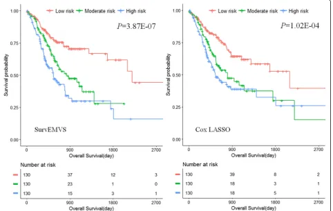
presents similar estimations with its counterpart in the low-dimensional Weibull regression. According to tertiles of risk scores, we equally divided the patients into high-, moderate-, and low-risk groups. Figure4presents the KM curves of SurvEMVS (left panel) and Cox LASSO (right panel), respectively, and both of them show a higher risk score which is significantly associated with shorter survival (Log-rank testP= 3.87E−07 for SurvEMVS andP= 1.02E

−04 for Cox LASSO).

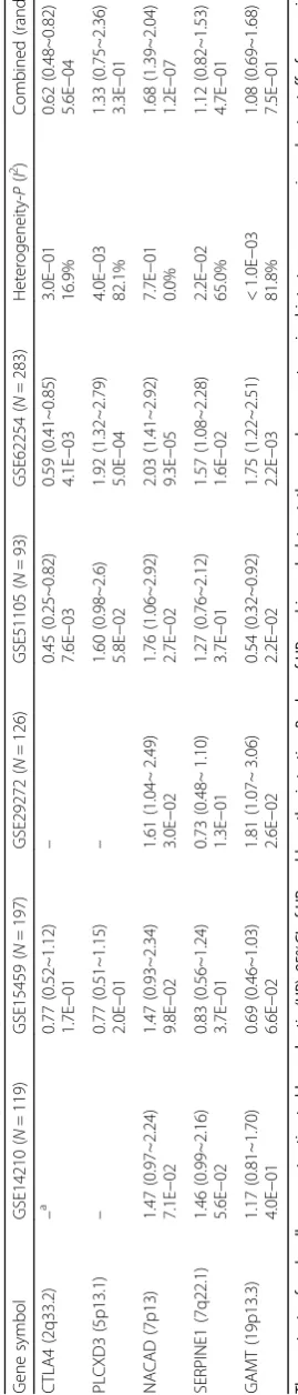
Furthermore, in order to validate the results, we used

external data from GEO database. Five datasets

(GSE14210, GSE15459, GES29272, GSE51105, and

GSE62254) are included for their proper sample sizes.

Table 4 presents the estimated hazard ratios along with

95% confidence intervals (CI) and P value extracted

from an online tool (KM plotter,Web resource). We also show the combined results using meta-analysis. As a re-sult, CTLA4 and NACAD were successfully validated and have the same direction of the effects on prognosis with those estimated by SurvEMVS in TCGA-STAD data. Interestingly, CTLA4 encodes CTLA-4 (cytotoxic T-lymphocyte-associated protein 4) which inhibits T cell activation and downregulates immune response. Antag-onistic antibody against CTLA has become a targeted drug (Ipilimumab, approved by FDA for melanoma in

2011), which is the first approved and popular immune

checkpoint blockade therapy [50, 51]. Some research

also indicates CTLA4 may have influence on gastric

can-cer germination and progression [52, 53]. GAMT and

PLCXD3 detected by Cox LASSO display strong hetero-geneity on effects (81.8% and 82.1%, respectively) with five datasets and no significant association in the com-bined analysis. Note that ALG11 is not identified in the five data. Although we acquire a negative consequence of SERPINE1 (also known as plasminogen activator inhibitor-1, PAI-1) in validation analysis; interestingly, it has been widely studied and is well known for participat-ing p53 signalparticipat-ing pathway and playparticipat-ing a crucial role in tumor progression and angiogenesis [54,55].

Discussion

High-throughput sequencing technology, which has be-come cheaper, promotes the development of precision medicine [56]. Picking up underlying markers affecting disease prognosis from thousands of candidates calls for high-dimensional survival model besides generally used one-by-one Cox proportional hazards model. In this paper, we propose a parametric survival counterpart of EMVS, namely SurvEMVS, which employs a fast EM al-gorithm to fit all candidate biomarkers simultaneously and to explore posterior distribution of the unknown pa-rameters, consequently to identify important signals and make effect estimations.

Much work has concentrated on developing new Bayes-ian methods on high-dimensional parametric survival model in application to medical or genetic data. For ex-ample, Sha et al. built AFT models with less common dis-tribution (i.e., log-normal and log-t) for microarray data using a discrete spike-and-slab prior, where a time-con-suming MCMC procedure was employed to simulate pos-terior distribution [57]. Mittal et al. developed four parametric models, i.e., exponential, Weibull, log-logistic, and log-normal distribution, by assigning Gaussian and Laplace prior to effects, where maximum a posterior (MAP) was used to acquire posterior modes of effects; however, this work lacked numerical study to evaluate their models, as well as discussion on variables selected in real data analysis from medical reasonability [58]. New-combe et al. imposed a discrete spike-and-slab prior on coefficients of Weibull regression, where reversible jump MCMC being used for the posterior computation is inef-fective. Moreover, it is unrepresentative of their applica-tion to a low-dimensional breast cancer data [59].

SurvEMVS imposes a continuous spike-and-slab mix-ture prior on effects to facilitate the separation of differ-ent effect sizes. This two-compondiffer-ent prior can provide an indicator vector to guide variable selection whereby using a local version of the median probability model [22, 60]. In contrast, the EM algorithm or variational

approximation employing one-component prior such as Laplace ortdistribution does not involve variable inclu-sion indicators, and consequently makes variable selec-tion indirectly [20]. Due to the unavailable closed form of maximization about maker effects in M-step, a variant of CCD algorithm serves to be feasible for obtaining ap-proximate solutions. Consequently, our EM steps in-corporating this fast CCD make the fitting much effective. One focus of this study is how to choose an optimal model from the hyperparameter tuning process. The EBIC, an extension of the BIC, is adopted with rea-son as follows: in comparirea-son with the EBIC, the nor-mally used AIC, BIC, or GCV would generate more spurious signal when applied to high-dimensional data, while CV-based metrics demand more computation and are unstable since the folds in CV are selected randomly. This is, to our knowledge, the first application of EBIC to the high-dimensional parametric survival analysis.

Over a range of simulation scenarios, our method with EBIC2 generally performs better than Cox LASSO in variable selection, parameter estimation, and prediction. In contrast, owing to imposing a single penalty on all ef-fects, Cox LASSO yields high biased estimators. Our simulations also show the EBIC is appropriate for model selection, while the BIC (i.e., EBIC1) perform worst in situation with very large number of markers. For p>n

problem in omics data, we recommend τ= 0.5 for EBIC

in multi-stage study because it offers a good trade-off between the well-controlled FDR and the TPR and pro-vides more opportunity to new findings. However, if one

is strict to control false discovery, τ= 1, is

recom-mended. Subsequently, we conducted two real data ap-plications. In the first study with a lung cancer genotype data, 14 SNPs were detected by SurvEMVS, and further validation analyses using external data or function anno-tation resulted in 7 outstanding SNPs. In order to widen the application range of SurvEMVS considerably, we uti-lized a stomach cancer expression data in the second study. Expression levels of three genes are associated with cancer prognosis, and two of them are validated by extra GEO datasets along with one (namely SERPINE1) involved in tumor progression. The identification of well-known CTLA4 illustrates the availability of Sur-vEMVS. However, further functional experiments are needed for evidence of biologic plausibility of those identified markers.

data application relative to a simulation study. We can explain that ideal conditions (e.g., sparse structure with independent markers) along with strong shrinkage of candidate hyperparameters (producing a parsimonious model) favor rapid convergence, but generally are not available under real data applications, which leads to more iterations demanding (but still fast enough) not only for SurvEMVS but also for other model [20].

However, we acknowledge that there are several limita-tions of the present study. First, SurvEMVS incorporating the EM, which seeks for a posterior mode rather than a whole posterior distribution of the parameter, cannot pro-vide uncertain measure for estimators. We can directly disentangle this disadvantage by the bootstrap method, but have to bear expensive computations. Actually, an-other compromise may be adopted: the estimates of Sur-vEMVS can be considered as initial values of a following MCMC algorithm, which makes the MCMC procedure avoid the burn-in stage and finally yield fast and accurate estimators with uncertain measurement. Second, the most worrying thing of the parametric model is a situation of going against the parametric assumption for survival dis-tribution. We show that SurvEMVS is robust for the sta-tus with moderately deviating from the Weibull premise. However, we believe that SurvEMVS will be less effective if the real survival time distinctly violates the Weibull dis-tribution. We can bypass this limitation using a

non-para-metric AFT model like in [61], in which a Dirichlet

process is used to make the model robust over a wider range of unknown baseline hazard. In addition, a lot of new directions for methodological work will arise from the current study. One obvious extension to our method will consider multivariate “g-priors” to reflect the effect correlations within the correlated markers [62]. Another interesting extension will involve introducing a newly de-veloped spike-and-slab Laplace prior [63]. Going forward, the meaningful extension of SurvEMVS will integrate functional annotations or multi-omics data to powerfully mine association signals in future work.

Conclusions

We present a new implementation of the EM algorithm for Bayesian variable selection under a Weibull survival model. Both of our simulation studies and two real data analyses show that the proposed method is effective and can cope with high-dimensional omics data.

Additional file

Additional file 1: Table S1.TPR, FPR and FDR in variable selection with

50 replications (Weibull distribution).Table S2.TPR, FPR and FDR in

variable selection with 50 replications (Gamma distribution).Table S3.

Computational time (minutes) for application in simulation trials.Table S4.

The estimated effects of 14 SNPs by SurvEMVS and classical Weibull

regression.Table S5.Demographic and clinical characteristics of STAD

patients.Table S6.The estimated effects of gene expression levels selected

by SurvEMVS and Cox LASSO with their counterparts in low dimension

scenario (i.e., Weibull regession and Cox model, respectively).Figure S1.

Pseudocode for implementation of SurvEMVS.Figure S2.Averaged

estimated effect (black vertical lines) for each marker over 50 replications

under Scenario 2.Figure S3.Averaged estimated effect (_{black vertical lines})

for each marker over 50 replications under Scenario 3.Figure S4.Averaged

estimated effect (_{black vertical lines}) for each marker over 50 replications

under Scenario 4.Figure S5.Averaged estimated effect (black vertical lines)

for each marker over 50 replications under Scenario 5.Figure S6Averaged

estimated effect (black vertical lines) for each marker over 50 replications

under Scenario 6.Figure S7.MSE of parameter estimation and AUC of

prognosis prediction for Scenarios 3 and 4.Figure S8.MSE of parameter

estimation and AUC of prognosis prediction for Scenarios 5 and 6.Figure S9.

Kaplan-Meier survival curve of patients with high, moderate, and low risk. (DOCX 9932 kb)

Abbreviations

AFT:Accelerated failure time; CCD: Cyclic coordinate descent; EBIC: Extended

Bayesian Information Criteria; EM: Expectation-maximization; GEO: Gene Expression Omnibus; LASSO: Least absolute shrinkage and selection operator; MCMC: Markov Chain Monte Carlo; TCGA: The Cancer Genome Atlas

Acknowledgements

We thank the participants and staff for their important contributions to this study.

Funding

This study was funded by National Natural Science Foundation of China (81530088 and 81473070 to F.C.), National Key Research and Development Program of China (2016YFE0204900 to F.C.), the National Institutes of Health (CA092824 and CA209414 to D.C.C.), Natural Science Foundation of the Jiangsu Higher Education Institutions of China (14KJA310002 to F.C.), Research and Innovation Project for College Graduates of Jiangsu Province of China (KYLX16_1123 to W.D.), Priority Academic Program Development of Jiangsu Higher Education Institutions (PAPD), and Top-notch Academic Pro-grams Project of Jiangsu Higher Education Institutions (TAPP:

PPZY2015A067). Y.W. and R.Z. were partially supported by the Outstanding Young Teachers Training Program of Nanjing Medical University.

Availability of data and materials

The first real dataset (i.e., Harvard lung cancer data) is available upon request. The second real dataset (i.e., TCGA stomach adenocarcinoma expression

data) can be found in TCGA database (_{Web resources}). The validation datasets

of gene expression are available at GEO database with accession numbers: GSE14210, GSE15459, GES29272, GSE51105, and GSE62254. The summary

statistics of the GEO data can be extracted from KM plotter (Web resources)

directly.

Web resources

TCGA:https://portal.gdc.cancer.gov/

UALCAN:http://ualcan.path.uab.edu/index.html

KEGG:http://www.kegg.jp/kegg/genes.html

KM plotter:http://www.kmplot.com/analysis/index.php?p=service

PLINK:http://www.cog-genomics.org/plink2

Authors’contributions

WD, RZ, FC, and DCC contributed to the conception and design. WD contributed to the development of methodology. YZ and DCC contributed to the acquisition of data. WD, RZ, YZ, YW, and SS contributed to the analysis and interpretation of data. WD, RZ, and FC contributed to the writing, review, and revision of the manuscript. All authors read and approved the final manuscript.

Ethics approval and consent to participate

Consent for publication

Not applicable.

Competing interests

The authors declare that they have no competing interests.

Publisher’s Note

Springer Nature remains neutral with regard to jurisdictional claims in published maps and institutional affiliations.

Author details

1

Department of Biostatistics, School of Public Health, Nanjing Medical University, 101 Longmian Avenue, Nanjing 211166, Jiangsu, China.2_China

International Cooperation Center for Environment and Human Health, Nanjing Medical University, 101 Longmian Avenue, Nanjing 211166, Jiangsu, China.3Joint Laboratory of Health and Environmental Risk Assessment (HERA), Nanjing Medical University School of Public Health / Harvard School of Public Health, 101 Longmian Avenue, Nanjing 211166, Jiangsu, China.4_Key

Laboratory of Biomedical Big Data of Nanjing Medical University, 101 Longmian Avenue, Nanjing 211166, Jiangsu, China.5Department of Environmental Health, Harvard School of Public Health, Boston, MA, USA.

6_{Pulmonary and Critical Care Division, Department of Medicine,}

Massachusetts General Hospital/Harvard Medical School, Boston, MA 02114, USA.

Received: 26 June 2018 Accepted: 7 October 2018

References

1. Metzker ML. Sequencing technologies - the next generation. Nat Rev Genet.

2010;11(1):31.

2. Veeramah KR, Hammer MF. The impact of whole-genome sequencing

on the reconstruction of human population history. Nat Rev Genet. 2014;15(3):149.

3. Network TCGA. Comprehensive molecular characterization of gastric

adenocarcinoma. Nature. 2014;513(7517):202–9.

4. Edgar R, Domrachev M, Lash AE. Gene expression omnibus: NCBI gene

expression and hybridization array data repository. Nucleic Acids Res. 2002;

30(1):207–10.

5. Yang J, Lee SH, Goddard ME, Visscher PM. GCTA: a tool for genome-wide

complex trait analysis. Am J Hum Genet. 2011;88(1):76–82.

6. Hu Z, Wu C, Shi Y, Guo H, Zhao X, Yin Z, Yang L, Dai J, Hu L, Tan W. A

genome-wide association study identifies two new lung cancer

susceptibility loci at 13q12.12 and 22q12.2 in Han Chinese. Nat Genet. 2011;

43(8):792–6.

7. Dong J, Hu Z, Wu C, Guo H, Zhou B, Lv J, Lu D, Chen K, Shi Y, Chu M.

Association analyses identify multiple new lung cancer susceptibility loci and their interactions with smoking in the Chinese population. Nat Genet. 2012;44(8):895.

8. Zhou X, Stephens M. Genome-wide efficient mixed model analysis for

association studies. Nat Genet. 2012;44(7):821.

9. Chen H, Wang C, Conomos MP, Stilp AM, Li Z, Sofer T, Szpiro AA, Chen W,

Brehm JM, Celedón JC. Control for population structure and relatedness for binary traits in genetic association studies via logistic mixed models. Am J

Hum Genet. 2016;98(4):653–66.

10. Yang J, Zaitlen NA, Goddard ME, Visscher PM, Price AL. Advantages and

pitfalls in the application of mixed-model association methods. Nat Genet.

2014;46(2):100_–6.

11. Guan Y, Stephens M. Bayesian variable selection regression for

genome-wide association studies and other large-scale problems. Ann Appl Stat.

2011;5(3):1780–815.

12. Moser G, Sang HL, Hayes BJ, Goddard ME, Wray NR, Visscher PM.

Simultaneous discovery, estimation and prediction analysis of complex traits using a Bayesian mixture model. PLoS Genet. 2015;11(4):e1004969.

13. Tibshirani R. Regression shrinkage and selection via the lasso: a

retrospective. J R Stat Soc B. 2011;73:273_–82.

14. Zou H. The adaptive lasso and its oracle properties. J Am Stat Assoc. 2006;

101(476):1418–29.

15. Casella TP, George. The Bayesian lasso. J Am Stat Assoc. 2008;103(482):681–6.

16. George EI, Mcculloch RE. Approaches for Bayesian variable selection. Stat

Sin. 1997;7(2):339–73.

17. Zhou X, Carbonetto P, Stephens M. Polygenic modeling with Bayesian

sparse linear mixed models. PLoS Genet. 2013;9(2):e1003264.

18. Carbonetto P, Stephens M. Scalable variational inference for Bayesian

variable selection in regression, and its accuracy in genetic association

studies. Bayesian Anal. 2012;7(1):73_–107.

19. Logsdon BA, Carty CL, Reiner AP, Dai JY, Kooperberg C. A novel variational

Bayes multiple locus Z-statistic for genome-wide association studies with Bayesian model averaging. Bioinformatics. 2012;28(13):1738.

20. Duan W, Zhao Y, Wei Y, Yang S, Bai J, Shen S, Du M, Huang L, Hu Z, Chen F.

A fast algorithm for Bayesian multi-locus model in genome-wide

association studies. Mol Gen Genet. 2017;292(4):923–34.

21. Hayashi T, Iwata H. EM algorithm for Bayesian estimation of genomic

breeding values. BMC Genet. 2010;11(1):3.

22. Ročková V, George EI. EMVS: the EM approach to Bayesian variable

selection. J Am Stat Assoc. 2014;109(506):828–46.

23. Oakes D. Biometrika centenary: survival analysis. Biometrika. 2001;88(1):99_–142.

24. Ziegel ER. Modelling for survival data in medical research by D. Collett:

Chapman & Hall; 1994.

https://www.crcpress.com/Modelling-Survival-Data-in-Medical-Research-Third-Edition/Collett/p/book/9781439856789.

25. Hosmer DW, Lemeshow S. Applied survival analysis: regression modeling of

time to event data: Wiley-Interscience; 1999.https://www.wiley.com/en-us/

Applied+Survival+Analysis%3A+Regression+Modeling+of+Time+to+Event +Data%2C+2nd+Edition-p-9780471754992.

26. Cox DR. Regression models and life-tables: Springer New York; 1992.https://

link.springer.com/chapter/10.1007%2F978-1-4612-4380-9_37.

27. Keiding N, Andersen PK, Klein JP. The role of frailty models and accelerated

failure time models in describing heterogeneity due to omitted covariates.

Stat Med. 1997;16(1–3):215.

28. Robins JM, Scheines R, Spirtes P, Wasserman L. A Bayesian justification of

Cox’s partial likelihood. Biometrika. 2003;90(3):629–41.

29. Zucknick M, Saadati M, Benner A. Nonidentical twins: comparison of

frequentist and Bayesian lasso for Cox models. Biom J. 2015;57(6):959–81.

30. Klein JP, Moeschberger ML. Survival analysis: techniques for censored and

truncated data. 2nd ed; 2003.

31. Dempster AP, Laird NM, Rubin DB. Maximum likelihood from incomplete

data via the EM algorithm. J R Stat Soc. 1977;39(1):1_–38.

32. Luenberger DG, Ye Y. Linear and nonlinear programming: Addison-Wesley; 1984.

https://link.springer.com/book/10.1007%2F978-0-387-74503-9.

33. Tong Z, Oles FJ. Text categorization based on regularized linear

classification methods. Inf Retr. 2001;4(1):5–31.

34. Genkin A, Lewis DD, Madigan D. Large-scale Bayesian logistic regression for

text categorization. Technometrics. 2007;49(3):291–304.

35. Simon N, Friedman J, Hastie T, Tibshirani R. Regularization paths for Cox’s

proportional hazards model via coordinate descent. J Stat Softw. 2011;39(05):1_–13.

36. Van Houwelingen HC, Bruinsma T, Hart AAM, Van'T Veer LJ, Wessels LFA.

Cross-validated cox regression on microarray gene expression data. Stat Med. 2006;25(18):3201.

37. Bogdan M, Ghosh JK, Doerge RW. Modifying the Schwarz Bayesian

information criterion to locate multiple interacting quantitative trait loci.

Genetics. 2004;167(2):989–99.

38. Siegmund D. Model selection in irregular Problems: applications to

mapping quantitative trait loci. Biometrika. 2004;91(4):785_–800.

39. Chen J, Chen Z. Extended Bayesian information criteria for model selection

with large model spaces. Biometrika. 2008;95(3):759–71.

40. Jr HF, Lee KL, Mark DB. Multivariable prognostic models: issues in

developing models, evaluating assumptions and adequacy, and measuring

and reducing errors. Stat Med. 1996;15(4):361–87.

41. Purcell S, Neale B, Todd-Brown K, Thomas L, Ferreira MAR, Bender D, Maller

J, Sklar P, Bakker PIWD, Daly MJ. PLINK: a tool set for whole-genome association and population-based linkage analyses. Am J Hum Genet. 2007;

81(3):559–75.

42. Asomaning K, Miller DP, Liu G, Wain JC, Lynch TJ, Su L, Christiani DC.

Second hand smoke, age of exposure and lung cancer risk. Lung Cancer. 2008;61(1):13.

43. Machida EO, Brock MV, Hooker CM, Nakayama J, Ishida A, Amano J, Picchi

MA, Belinsky SA, Herman JG, Taniguchi S. Hypermethylation of ASC/TMS1 is a sputum marker for late-stage lung cancer. Cancer Res. 2006;66(12):6210.

44. Zhao Y, Wei Q, Hu L, Chen F, Hu Z, Heist RS, Su L, Amos CI, Shen H,

Christiani DC. Polymorphisms in MicroRNAs are associated with survival in non-small cell lung cancer. Cancer Epidemiol Biomarkers Prev. 2014;23(11):

45. Chandrashekar DS, Bashel B, Sah B, Creighton CJ, Ponce-Rodriguez I, Bvsk C, Varambally S. UALCAN: a portal for facilitating tumor subgroup gene expression and survival analyses. Neoplasia. 2017;19(8):649.

46. Brabender J, Danenberg KD, Metzger R, Schneider PM, Lord RV, Groshen S,

Tsao-Wei DD, Park J, Salonga D, Holscher AH, et al. The role of retinoid X receptor messenger RNA expression in curatively resected non-small cell

lung cancer. Clin Cancer Res. 2002;8(2):438_–43.

47. He S, Chen CH, Chernichenko N, He S, Bakst RL, Barajas F, Deborde S, Allen

PJ, Vakiani E, Yu Z. GFRα1 released by nerves enhances cancer cell

perineural invasion through GDNF-RET signaling. Proc Natl Acad Sci U S A. 2014;111(19):E2008.

48. Colaprico A, Silva TC, Olsen C, Garofano L, Cava C, Garolini D, Sabedot

TS, Malta TM, Pagnotta SM, Castiglioni I. TCGAbiolinks: an R/ Bioconductor package for integrative analysis of TCGA data. Nucleic Acids Res. 2016;44(8):e71.

49. White IR, Royston P, Wood AM. Multiple imputation using chained

equations: issues and guidance for practice. Stat Med. 2011;30(4):377–99.

50. Pardoll DM. The blockade of immune checkpoints in cancer

immunotherapy. Nat Rev Cancer. 2012;12(4):252_–64.

51. Wei SC, Levine JH, Cogdill AP, Zhao Y, Anang NAS, Andrews MC,

Sharma P, Wang J, Wargo JA, Pe'er D, et al. Distinct cellular mechanisms underlie anti-CTLA-4 and anti-PD-1 checkpoint blockade.

Cell. 2017;170(6):1120–1133.e1117.

52. Hou R, Cao B, Chen Z, Li Y, Ning T, Li C, Xu C, Chen Z. Association of

cytotoxic T lymphocyte-associated antigen-4 gene haplotype with the

susceptibility to gastric cancer. Mol Biol Rep. 2010;37(1):515–20.

53. Kim JW, Nam KH, Ahn SH, Park DJ, Kim HH, Kim SH, Chang H, Lee JO, Kim

YJ, Lee HS, et al. Prognostic implications of immunosuppressive protein expression in tumors as well as immune cell infiltration within the tumor

microenvironment in gastric cancer. Gastric Cancer. 2016;19(1):42–52.

54. Rakic JM, Maillard C, Jost M, Bajou K, Masson V, Devy L, Lambert V, Foidart

JM, Noel A. Role of plasminogen activator-plasmin system in tumor

angiogenesis. Cell Mol Life Sci. 2003;60(3):463–73.

55. Takayama Y, Hattori N, Hamada H, Masuda T, Omori K, Akita S, Iwamoto H,

Fujitaka K, Kohno N. Inhibition of PAI-1 limits tumor angiogenesis regardless of angiogenic stimuli in malignant pleural mesothelioma. Cancer Res. 2016; 76(11):3285.

56. Collins FS, Varmus H. A new initiative on precision medicine. N Engl J Med.

2015;372(9):793.

57. Sha N, Tadesse MG, Vannucci M. Bayesian variable selection for the analysis

of microarray data with censored outcomes. Bioinformatics. 2006;22(18):

2262–8.

58. Mittal S, Madigan D, Cheng JQ, Burd RS. Large-scale parametric survival

analysis. Stat Med. 2013;32(23):3955_–71.

59. Newcombe P, Raza AH, Blows F, Provenzano E, Pharoah P, Caldas C,

Richardson S. Weibull regression with Bayesian variable selection to identify prognostic tumour markers of breast cancer survival. Stat Methods Med Res. 2014;26(1):414.

60. Barbieri M, Berger J. Optimal predictive model selection. Ann Stat. 2004;

32(3):870_–97.

61. Zhang Z, Sinha S, Maiti T, Shipp E. Bayesian variable selection in the

accelerated failure time model with an application to the surveillance, epidemiology, and end results breast cancer data. Stat Methods Med Res.

2016.https://doi.org/10.1177/0962280215626947.

62. Zellner A. On assessing prior distributions and Bayesian regression analysis

with G-prior distributions. Bayesian Inference Decis Tech. 1986;6:233–43.

63. Ročková V, George EI. The Spike-and-Slab LASSO. J Am Stat Assoc. 2018;

113(521):431–44.https://doi.org/10.1080/01621459.2016.1260469.

64. Gao AC, Lou W, Isaacs JT. Enhanced GBX2 expression stimulates growth of

human prostate cancer cells via transcriptional up-regulation of the

interleukin 6 gene. Clin Cancer Res. 2000;6(2):493–7.

65. Gao AC, Lou W, Isaacs JT. Down-regulation of homeobox gene GBX2

expression inhibits human prostate cancer clonogenic ability and tumorigenicity. Cancer Res. 1998;58(7):1391.

66. Nimmrich I, Erdmann S, Melchers U, Chtarbova S, Finke U, Hentsch S,

Hoffmann I, Oertel M, Hoffmann W, Müller O. The novel ependymin related gene UCC1 is highly expressed in colorectal tumor cells. Cancer Lett. 2001;

165(1):71–9.

67. Liu Z, Zhang J, Gao Y, Pei L, Zhou J, Gu L, Zhang L, Zhu B, Hattori N,

Ji J. Large-scale characterization of DNA methylation changes in human

gastric carcinomas with and without metastasis. Clin Cancer Res. 2014;

20(17):4598_–612.

68. Godinheymann N, Brabetz S, Murillo MM, Saponaro M, Santos CR, Lobley A,

East P, Chakravarty P, Matthews N, Kelly G. Tumour-suppression function of KLF12 through regulation of anoikis. Oncogene. 2015;35(25):3324.

69. Yu N, Migita T, Hosoda F, Okada N, Gotoh M, Arai Y, Fukushima M, Ohki M,

Miyata S, Takeuchi K. Krüppel-like factor 12 plays a significant role in poorly differentiated gastric cancer progression. Int J Cancer. 2009;125(8):1859.

70. Rozenblum E, Vahteristo P, Sandberg T, Bergthorsson JT, Syrjakoski K,

Weaver D, Haraldsson K, Johannsdottir HK, Vehmanen P, Nigam S, et al. A genomic map of a 6-Mb region at 13q21-q22 implicated in cancer development: identification and characterization of candidate genes. Hum