“thorough QT/QTc study”
Suraj P. Anand
∗and Sujit K. Ghosh
Department of Statistics, North Carolina State University, Raleigh,
North Carolina, USA
Institute of Statistics Mimeo Series 2610
Abstract
The standard methods for analyzing data arising from a ‘thorough QT/QTc study’ are based on
multivariate normal models with common variance structure for both drug and placebo. Such modeling
assumptions may be violated and when the sample sizes are small the statistical inference can be sensitive
to such stringent assumptions. This article proposes a flexible class of parametric models to address the
above mentioned limitations of the currently used models. A Bayesian methodology is used for data
analysis and models are compared using the deviance information criteria (DIC). Superior performance
of the proposed models over the current models is illustrated through a real data set obtained from a
GlaxoSmithKline conducted ‘thorough QT/QTc study’.
1
Introduction
QT prolongation is an important issue in clinical safely of already marketed and investigational new drugs.
It is an undesirable property associated with some non-antiarrhythmic drugs due to their ability to delay
cardiac repolarization, more generally known as QT prolongation. The QT interval is a segment of the
surface electrocardiogram (ECG) and represents the duration of ventricular depolarization and subsequent
repolarization, and is measured from the beginning of the QRS complex to the end of the T wave. QT values
are correlated with heart rate and hence a corrected version (QTc) is used for data analysis (see International
Conference of Harmonization (ICH) E14 guidelines, available atwww.fda.gov/cder/guidance/). The ICH
∗Correspondence: Suraj Anand, Department of Statistics, North Carolina State University, Raleigh, NC 27695-8203, USA;
E-mail: [email protected]
E14 guidelines recommend conducting a ‘thorough QT/QTc study’ to determine whether the drug has a
threshold pharmacological effect on cardiac repolarization, as detected by QTc prolongation. The study
is typically carried out in healthy volunteers and is used to determine whether or not the effect of a drug
on the QTc interval in target patient populations should be studied intensively during later stages of drug
development.
Measurements taken in a QT study are naturally in time order, with multiple QTc measurements
taken on each subject at a number of time-points, hence the comparison of drug with placebo involves
assessing the time-matched differences at each of those time-points. The standard approach to analyzing
QT data to assess a drug for a potential QT prolongation effect is driven by an intersection-union testing
approach. This is performed by constructing a 90% two-sided (or a 95% one-sided) confidence interval (CI),
for the time-matched mean difference in baseline corrected QTc between drug and placebo at each time-point,
and concluding non-inferiority if the upper limits for all these CIs are less than 10 ms. A positive control
known to have a QT prolonging effect is also included to assess the sensitivity of the study in detecting the
QT effects. Under the standard normality assumptions, the intersection-union test based standard approach
is known to be conservative and biased (Patterson and Jones, 2005).
According to the The ICH E14 guidelines, a negative ‘thorough QT/QTc Study’ is one in which the
upper bound of the 95% one-sided confidence interval for the largest time-matched mean effect of the drug on
the QTc interval excludes 10 ms. When the largest time-matched mean difference exceeds the threshold, the
study is termed positive. Hence, instead of constructing confidence intervals at each of the time-points , one
could base the non-inferiority inference on an interval estimate for the largest time-matched mean difference
in QTc between drug and placebo. Constructing such an interval estimate for the maximum difference,
which is a non-smooth function, however is a non-trivial task.
Few notable attempts to address this problem include newer approaches proposed by Eaton et
al. (2006), Boos et al. (2007), and Anand and Ghosh (2008). The method proposed by Eaton et al.
(2006) involves constructing asymptotic confidence interval for the parameter of maximum difference by
approximating it with a smooth function and then using the ‘delta method’ to obtain an approximate
confidence interval. In another study, Boos et al. (2007) proposed new bounds for the maximum difference,
obtained analytically and uses an expression for the approximate moments of the maximum of random
variables. Their second upper bound is based on a parametric bootstrap, bias-corrected percentile method,
whereas their third upper bound is based on a non-parametric bootstrap, bias-corrected percentile method.
Recently, Anand and Ghosh (2008) proposed a Bayesian approach to solving this problem. Their approach
involves constructing an interval estimate for the maximum difference based on the derived samples from the
posterior density of the maximum difference. They use normal conjugate priors for the mean vectors and
inverse wishart prior for the common covariance matrix to derive the closed form posterior density for the
population mean vectors and covariance matrix, and employ a Monte Carlo sampling technique to sample
from the posterior density of the maximum difference. Their proposed approach is based on finite sample
and does not make use of any asymptotic approximations.
All the above methods are based on multivariate normal models for the QT data with common
covariance structure for both drug and placebo. Such modeling assumptions may not be reasonable in all
situations and may need to be relaxed to reflect observed data. These assumptions may be violated and
when the sample sizes are small the statistical inference about the maximum time-matched mean difference
parameter can be sensitive to such stringent assumptions. In this Chapter, we propose a flexible class of
parametric models to address the above mentioned limitations of the currently used models. A Bayesian
methodology is used for data analysis and we compare the models using the deviance information criteria
(DIC). We illustrate the superior performance of the proposed models over the current models through a
real data set obtained from a GSK conducted Thorough QT study. We lay out a flexible class of multivariate
models suitable for the QTc data in Section 2. In Section 3, we provide details for the model comparisons
and analysis methods. In Section 4 we apply the proposed method to a real data set on QTc obtained from
a thorough QT study run at GlaxoSmithKline (GSK). We compare different models using the DIC criterion
and provide analysis results for the preferred model. Finally, We present the concluding remarks and a
2
A Flexible Class of Models for QTc Data
We develop a general statistical model for the parallel study design for QTc data. Letn1andn2denote the
number of subjects receiving drug and placebo respectively, with baseline corrected QTc values calculated
atptime points. We denote the vector ofpmeasurements taken on the subjects on drug byxi, i= 1, . . . n1,
and those on control by yj, j = 1, . . . n2, respectively. The commonly used models for QTc data are all
based on the assumptions of normality and common covariance structure for drug and placebo but we allow
a much more flexible class of multivariatet models in all its generality. We assume that the measurements are distributed identically and independently (iid), arising from two independentp-variate tdistributions as follows:
xi iid
∼ tν1(µ1,Σ1), i= 1, . . . , n1, and
yj iid
∼ tν2(µ2,Σ2), j= 1, . . . , n2, (1)
whereµ1andµ2are the population means for the drug and placebo groups, respectively, and the dispersion
matricesΣ1andΣ2are assumed to be unknown and unstructured. We denote byδ=µ1−µ2, the vector of
time-matched mean differences in mean QTc between drug and placebo. ν1>2 andν2>2 are the degrees
of freedom for the respectivetdistributions. The parameter of interest is the maximum time-matched mean difference between the two groups and we denote it byθ,
θ= max
1≤k≤pδk ≡1max≤k≤p(µ1k−µ2k). (2)
It is well known that as the degrees of freedom get large νk → ∞ for k= 1,2, the multivariate t
distribution approaches to a multivariate normal distribution and hence this flexible class of models includes
the commonly used multivariate models for the QTc data.
The primary objective of a QT study is to obtain an interval estimate forθ. It is easy to see thatθis a non-smooth function ofµ1andµ2and hence we can not apply the delta-method (Casella and Berger, 2002,
p.245) based on the moment estimates ˆµ1= ¯xand ˆµ2= ¯y, where ¯x= P
ixi/n1and ¯y=Pjyj/n2 denote
priors for this general class of models. So, depending on the prior specifications on µ1,µ2, Σ1 and Σ2,
the respective posterior densities are analytically intractable but we can still sample from these posterior
distributions using Markov Chain Monte Carlo (MCMC) sampling techniques. It should be noted that even
with the simpler Multivariate normal model, for which a class of conjugate priors exists for (µ1,µ2,Σ), where Σ is the common covariance matrix (Σ1 = Σ2 =Σ), it is still almost impossible to obtain the posterior
distribution of θ analytically and one has to employ a Monte Carlo sampling method to generate samples from this posterior distribution (Anand and Ghosh, 2008 ).
In order to obtain the posterior distribution ofθwe first specify a class of priors forµ1,µ2,Σ1 and Σ2. A suitable class of priors for this model can be given as follows:
µ1 ∼ Np(µ10,Σ10),
µ2 ∼ Np(µ20,Σ20), Σ−1
1 ∼ Wp(k,R10) and
Σ−21 ∼ Wp(k,R20), (3)
where Wp denotes a p-dimensional Wishart distribution with degrees of freedom k > p−1 and positive
definite scale matrixRj0, j= 1,2 (Anderson, 1984, p.245).
With this class of priors, the posterior distribution of (µ1,µ2,Σ1,Σ2), and henceθ, is not
analyti-cally tractable. So, one has to employ MCMC sampling techniques to generate samples from the posterior
distribution ofθand use them to construct an interval estimate forθ.
3
Model Comparison and Analysis Methodology
We start with the commonly used mutivariate normal model with a common covariance structure for drug
placebo, we perform Box’s M test (Box, 1949) on the estimated covariance matrices. To do this, we calculate
theU statistic given by the formulaU =−2(1−c1)lnM, where
lnM =1 2
k X
1
riln|Si| −
1 2 k X 1 ri
ln|Spl|,
c1= k X 1 1 ri − 1 Pk 1ri
2p 2
+ 3p−1 6(p+ 1)(k−1)
,
and Spl =
Pk
1riSi
Pk
1ri , where Si is the estimated covariance matrix for ith arm, ri =ni−1 is the degrees of
freedom associated with theitharm,pis the dimension of the data vector, andk= 2 is the number of arms. Under the normality assumption for the data, U follows a Chi square distribution with 1
2(k−1)p(p+ 1)
degrees of freedom (Box, 1949).
If the Box’s M test yields a significant result, we abandon the common covariance assumption,
otherwise we employ a model selection technique to select the better model. An objective criterion to
compare the models could be based on the ability of the model to best predict a replicate dataset which has
the same structure as that currently observed one, and hence we use the Deviance Information Criterion
(DIC) proposed by Spiegelhalter et. al., (2002), for model comparisons. We choose a model with the smallest
DIC among a collection of finitely many models. There is no set significance rule for preferring one model
over another using DIC but a difference of more than 10 might rule out the model with the higher DIC,
differences between 5 and 10 are substantial, and differences less than 5 need to be used with caution. These
suggested guidelines are available atwww.mrc-bsu.cam.ac.uk/bugs/winbugs/dicpage.shtml.
For the normal models, we employ the above mentioned scheme to decide whether the assumption
of a common covariance structure for drug and placebo is a reasonable one, and then use DIC to further
compare the models. We also use DIC to compare the multivariate normal andt models. For multivariate
t models, as we indicated above, putting priors on the degrees of freedom νk for k = 1,2 makes sampling
from the posterior distributions too difficult, so we assume thatν1=ν2=ν is fixed and treat it as a tuning
parameter. To select the appropriate ν, we calculate the DIC for a range of νs and choose the one that minimizes the DIC for the model. We also use the DIC to see how a change in prior information affects the
In the absence of a closed form posterior density for θ, we used the MCMC software Winbugs (WinBUGS, version 1.4.1; available at www.mrc-bsu.cam.ac.uk/bugs/winbugs/) for generating samples
from the posterior distribution ofµ1,µ2, Σ1 and Σ2, and hence θ. Upto three chains with different initial
values were used to diagnose convergence. Programming language R (available at www.r-project.org/)
was used to load data into Winbugs, perform data manipulations, call and execute Winbugs from R using
the R package R2WinBUGS (also available at www.r-project.org/). DIC for each model was computed
using WinBUGS. LetD(θ) =−2logf(x,y|θ) denote the deviance for the model whereθ= (µ1,µ2,Σ1,Σ2),
where f(x,y|θ) denotes the joint density of (x,y) given θ. If we denote by ˆD the point estimate of the deviance obtained by substituting in the posterior mean ¯θ=E[θ|x,y],
ˆ
D=−2logf(x,y|¯θ),
and by ¯Dthe posterior mean of the deviance ¯D=E[D(θ)|x,y], then the effective number of parameterspD
is given by
pD= ¯D−D.ˆ
DIC is then defined as
DIC= ¯D+pD= ˆD+ 2pD.
ˆ
Dgives a measure of goodness of fit of the model whereaspD evaluates a measure of model complexity. DIC
combines these two characteristics together to give a model assessing criterion in a way such that smaller
values indicate a better predictive ability of a model.
The samples generated from the posterior distribution ofθwere used to calculate the 95% quantile as an interval estimate for the maximum time-matched mean difference θ. Samples generated from the posterior distributions ofΣ1 and Σ2 were used to obtain the posterior mean covariance matrices for drug
4
Real Data Example, Analysis and Results
Change from baseline is the primary end-point of interest in a QT study, where baseline is defined according
to the study design, the dosing pattern and other study specific considerations.
Table 1: Data schematics for a typical QT study.
Subject Time (Hrs) 1 2 3 ... 24
1 Baseline QTc X1 X2 X3 ... X24
1 Post-Dose (Drug) Y1 Y2 Y3 ... Y24
1 Change from baseline (Drug) Y1-X1 Y2-Y1 Y3-X3 ... Y24-X24
2 Baseline QTc X1 X2 X3 ... X24
2 Post-Dose (Placebo) Y1 Y2 Y3 ... Y24
2 Change from baseline (Placebo) Y1-X1 Y2-Y1 Y3-X3 ... Y24-X24
Table 1 presents the data schematics of a typical QT study. Multiple (usually triplicate)
measure-ments are taken at baseline to provide a mean baseline measurement by averaging across the replicates.
Usually, a positive control that is known to have an increasing effect on the QTc interval is also included to
assess the sensitivity of the study in detecting the QT effects. If the positive control demonstrates an effect
as compared to placebo, then the assay is considered reasonably sensitive to detection of QTc prolongation.
We use the data previously analyzed by Anand and Ghosh, (2008) that were obtained from a GSK
conducted thorough QT study with placebo, a positive control (Moxifloxacin), and multiple drug
concen-tration arms for the study drug, with QTc (Bazett) measurements taken at baseline (mean of triplicates)
and multiple time-points (p= 10). Although the actual study design was crossover, only data from a single period of the entire dataset were used and only data on placebo and the positive control arm (called drug
henceforth) were included to mimic a parallel study design, with 36 subjects in each arm, for the purpose of
illustration. The end-point of interest was change from baseline QTc values and the parameter of interest
was maximum time-matched mean difference between drug and placebo for baseline corrected QTc. The
4.1
Robustness With Respect to Sampling Distribution
We focussed our attention to the models that are indicated above in Section 3. The first model (M1) is
the simplest model that assumes that the data for drug and placebo arise from two multivariate normal
populations with different means but the same covariance structure. This corresponds to the special case of
model (1) where Σ1 =Σ2 and ν1 =ν2 =∞. The second model (M2) again assumes that the data come
from multivariate normal populations, but with different covariance structures for drug and placebo. The
third model (M3) assumes that the data come from multivariatetdistributions with same and fixed degrees of freedom (df), ν1 =ν2 = 11, with same covariance structures for drug and placebo, whereas, the fourth
model (M4) is a variation of the third model with different covariance structures for drug and placebo.
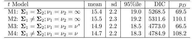
Table 2: Posterior summary statistics forθ using different models for the GSK data.
t Model mean sd 95%ile DIC pD
M1: Σ1=Σ2;ν1=ν2=∞ 15.4 2.2 19.0 5268.5 69.5
M2: Σ16=Σ2;ν1=ν2=∞ 15.5 2.3 19.2 5311.6 110.1
M3: Σ1=Σ2;ν1=ν2=ν∗ 14.9 2.2 18.5 4773.0 66.5
M4: Σ16=Σ2;ν1=ν2=ν 14.7 2.2 18.3 4784.9 108.2
*ν= 11 for the results provided in this table
We used Winbugs to generate a total of 15000 samples from the posterior distribution of µ1,µ2, Σ1 andΣ2, and hence θ followed by a burnin of 15000 samples based on three parallel chains. We used a class of normal priors forµ1,µ2 with the hyperparametersµj0= 0 for j = 1,2 and Σj0= 10
2
Ip, j = 1,2,
and an inverted wishart prior forΣj with the hyperparametersk=p+ 2 andRj0=Ip forj= 1,2. Data
and the intial values were loaded into Winbugs using R, and Winbugs execution was performed using the R
package R2WinBUGS. DIC andpD for each model were computed using Winbugs. The samples generated
from the posterior distribution ofθ for the above mentioned models were used to construct an upper 95% interval estimate (95% quantile) for the maximum time-matched mean differenceθ. Samples generated from the posterior distributions of Σ1 and Σ2 were used to obtain the posterior mean covariance matrices for
drug and placebo, and these estimates were used to check the common covariance assumption using Box’s M
5 10 15 20 25
0.00
0.05
0.10
0.15
0.20
0.25
0.30
θ
density
o ^ * o
normal − same sigma normal − different sigma t − same sigma t − different sigma
Figure 1: Posterior Density Plots forθfor different models
Looking at the summary statistics presented in Table 2 and Figure 1, it appears that even a change
in distributional assumptions for the data does not have a significant impact on the inference for θ. The means, standard deviations, and the 95% quantiles forθfor the multivariatetmodels (models M3 and M4) are slightly lower than that for the multivariate normal models (models M1 and M2), but the difference is
not substantial. Thus, the inference forθappears to be reasonably robust against changes to distributional assumptions for the data.
It is easy to see that the DIC is much larger for the multivariate normal models (M1 and M2) as
compared to the multivariatetmodels (M3 and M4), which indicates that, based on the minimum expected predictive error criterion as indicated by a lower DIC, the multivariate t models are expected to perform better than the multivariate normal models for the given data. Between the two multivariate t models, the one with same covariance structure for both drug and placebo outperforms the t model with different covariance structures. To ascertain the validity of the assumption of same covariance structure for drug and
placebo, we performed Box’s M test on the estimated covariance matrices as explained in Section 3. The
50.18 and 45.08 respectively, which when compared with the critical valueχ2
55,0.05= 73.31 suggest that the
assumption of a common covariance structure seems reasonable. These results indicate that a multivariatet
model with fixed degrees of freedom and same covariance structure seems to be the most appropriate choice
for the data. So, we proceeded to further investigate model M3 in greater details.
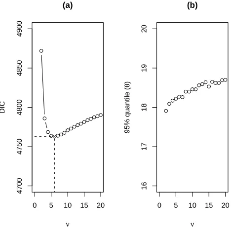
In models M3 and M4, we fixed degrees of freedomν= 11 as an initial guess to check the performance of thetmodels. To make a DIC-based selection of the degrees of freedom (df) for model M3, we calculated the DIC for a range of νs and chose the one that minimizes the DIC for model M3. Figure 2 (a) presents a plot of DIC vs. ν for this model. It can be seen that the DIC decreases with df until ν = 6, and then increases consistently with df. We also present a plot for the 95% quantile forθ vs. ν in Figure 2 (b). The plot suggests that the 95% quantile forθ is not affected much by a change inν. This suggests thatν = 6 is the most appropriate choice for model M3 according to the DIC criterion. Table 3 presents the results for
the multivariatetmodel withν = 6 and same covariance structure for drug and placebo.
0 5 10 15 20
4700
4750
4800
4850
4900
(a)
ν
DIC
0 5 10 15 20
16
17
18
19
20
(b)
ν
95% quantile (
θ
)
Table 3: Posterior summary statistics forθusing model M3 withν = 6.
Model mean sd 95%ile DIC pD
M3∗: Σ1=Σ2;ν
1=ν2= 6 14.7 2.2 18.3 4762.8 67.9
4.2
Robustness With Respect to Prior Specifications
After ascertaining the robustness of our methodology for distributional assumptions for the data, it was also
of interest to see how changes to prior information affect the results. To do this, we first investigated the
sensitivity of our methodology to the hyperparameterkthat appears to have a significant effect on the DIC of the model. We calculated the DIC for a range of values ofkfor model M3∗(withν = 6) as selected above.
Figure 3 (a) presents a plot of DIC vs. kfor this model. It can be seen that the DIC slowly decreases with
k until k = 17 and then shoots up rapidly. This suggests thatk = 17 is the most appropriate choice for model M3 according to the DIC criterion. Even though the DIC increases rapidly with k, the inference for
θ does not change sharply. For example, the 95% quantile forθ fork= 12 is 18.3 as compared to 18.0 for
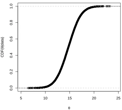
k = 40, and the two numbers are not too different for regulatory decisions. This shows that even though the predictive ability of the model decreases with an increase ink, the inference forθremains robust to this change. Table 4 presents the results fork= 17 and few extreme values ofk. We also present a plot for the 95% quantile for θvs. k in Figure 3 (b). It can be seen from the plot that the 95% quantile forθ initially decreases marginally with k but then stabilizes. According to the DIC criterion we chose k = 17 as our best choice for the hyperparameterk. We present a plot of the posterior cummulative distribution function (CDF) for this model in Figure 4.
Table 4: Posterior summary statistics forθfor model M3 withν= 6 for different values of the hyperparameter
k.
k mean sd 95%ile DIC
12 14.7 2.2 18.3 4762.8
17 14.7 2.1 18.2 4753.4
25 14.8 2.0 18.1 4784.5
50 15.0 1.9 18.0 8252.0
15 25 35
4500
5000
5500
6000
(a)
k
DIC
15 25 35
16
17
18
19
20
(b)
k
95% quantile (
θ
)
Figure 3: For model M3∗, panel (a) presents DIC vs. kand panel (b) presents the 95% posterior quantile of
θvs. k, where kis the prior parameter defined in (3.3)
5 10 15 20 25
0.0
0.2
0.4
0.6
0.8
1.0
θ
CDF(
θ
|data)
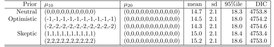
do this, we analyzed the data for several plausible combinations of the prior mean vectorsµ1andµ2. Table
5 summarizes these results. It can be seen that the results for neutral, optimistic, and skeptic priors do
not differ significantly. The posterior means are slightly different but the DIC and the statistic of interest,
posterior 95% quantile forθ, are close to each other. Thus, our methodology appears to be reasonably robust to the specification of the prior means.
These results together show that our t model as selected above using the DIC criterion is fairly robust to the distributional assumptions and prior specifications.
Table 5: Posterior summary statistics forθ(model M3) withν = 6 andk= 17 for different prior specifications on population means.
Prior µ10 µ20 mean sd 95%ile DIC
Neutral (0,0,0,0,0,0,0,0,0,0) (0,0,0,0,0,0,0,0,0,0,0) 14.7 2.1 18.3 4753.8 Optimistic (-1,-1,-1,-1,-1,-1,-1,-1,-1,-1) (0,0,0,0,0,0,0,0,0,0,0) 14.5 2.1 18.0 4754.2 (-2,-2,-2,-2,-2,-2,-2,-2,-2,-2) (0,0,0,0,0,0,0,0,0,0,0) 14.3 2.1 18.0 4754.6 Skeptic (1,1,1,1,1,1,1,1,1,1) (0,0,0,0,0,0,0,0,0,0,0) 15.0 2.1 18.4 4753.4 (2,2,2,2,2,2,2,2,2,2) (0,0,0,0,0,0,0,0,0,0,0) 15.2 2.1 18.6 4753.0
5
Conclusion and Discussion
The standard way of analyzing QT data involves comparing the 90% two-sided confidence intervals for the
time-matched mean differences to the regulatory threshold of 10 ms at each time-point, and is overly
conser-vative. Anand and Ghosh (2008) proposed a Bayesian approach to solving this problem by constructing an
interval estimate for the maximum of the time-matched mean differencesθbased on the derived samples from its posterior density. This method, along with few other recently proposed methods, assumes multivariate
normality with a common covariance structure, which may be violated with small sample sizes. We have
proposed a flexible class of multivariatetmodels that includes the ubiquitous multivariate normal model for such data. We have compared these models using the DIC criterion that evaluates a model on the basis of
its posterior predictive error.
We have gone in a methodical way to select the best model and then we show the robustness of
the given dataset, the DIC driven selection yields a small estimate for degrees of freedom (ν = 6) which indicates that a multivariate normal model may not be a good fit for the data. A large estimate forν would make the multivariate normality assumption more reliable. This methodology also gives us a way to check
the applicability of the assumption of a common covariance structure for drug and placebo. A DIC-based
criterion for the selection of the hyperparameterk helps in discarding models with poor predictive abilities. The flexibility to run the analysis for different specifications for the prior mean vectorsµ1 andµ2 enables
one to guard against the worst case scenario with a skeptic prior when the historical data suggest that the
drug prolongs QTc.
There does not seem to be an easy way of analyzing the QT data using a frequentist approach when
the normality assumption of the likelihood is questionable. Even when the multivariate normal likelihood
assumption is reasonable, the analysis using frequentist methods is not straightforward when the covariance
structures for drug and placebo are different. We have provided a flexible class of models for the QT data
and a sound mechanism for model building and analysis for such a data using a Bayesian approach. With the
MCMC sampling capabilities of Wingbugs the analysis is easy to perform with standard software without
relying on any kind of approximations or large sample theory assumptions.
References
Anand, S. P. and Ghosh, S. K. (2008). A Bayesian methodology for investigating the risk of QT
prolonga-tion,Journal of Statistical Theory and Practice, (In review).
Boos, D., Hoffman, D., Kringle, R., Zhang, J. (2007). New confidence bounds for QT studies,Statist. Med.,
26, 3801-3817.
Box, G. E. P. (1949). A General Distribution Theory for a Class of Likelihood Criteria, Biometrika 36,
317-346.
Casella, G. and Berger, R. L. (2002). Statistical inference, Duxbury Press.
Eaton, M. L., Muirhead, R. J., Mancuso, J. Y., Lolluri, S. (2006). A confidence interval for the maximal
International Conference on Harmonisation (2005). Guidance for Industry: E14 Clinical Evaluation of
QT/QTc Interval Prolongation and Proarrythmic Potential for Non-Antiarrythmic Drugs.
Available at: www.fda.gov/cber/gdlns/iche14qtc.htm
Patterson, S. (2005). Investigating Drug-Induced QT and QTc Prolongation in the Clinic: A Review
of Statistical Design and Analysis Considerations: Report from the Pharmaceutical Research and
Manufacturers of America QT Statistics Expert Team, Drug Inf J.,9, 243-266.
Patterson, S., Jones, B. Zariffa, N. (2005). Modeling and interpreting QTc prolongation in clinical
phar-macology studies,Drug Inf J.,39, 437-445.
Patterson S. and Jones B. (2005) Bioequivalence and Statistics in Clinical Pharmacology, Chapman and
Hall, CRC Press; London.
Spiegelhalter, D. J., Best, N. G., Carlin, B. P., and Van der Linde, A.(2002). Bayesian Measures of Model
Complexity and Fit (with Discussion), Journal of the Royal Statistical Society, Series B,64(4),