Coupled vs Uncoupled Reactor Building / Reactor Coolant System Seismic Analysis - A Short Review

Coupled vs Uncoupled Reactor Building / Reactor Coolant System Seismic Analysis – A Short Review

Nicolas JOBERT, Philippe MONETTE

AREVA-NP, Primary Components Department, Courbevoie, FRANCE

ABSTRACT

In nuclear industry, high attention is paid to robustness of heavy components structural analysis, of which the seismic loading may be a significant contributor.

During the analysis of the seismic structural motion, it is common practice to uncouple the Reactor Building and the Re-actor Coolant System dynamic analyses. This results in interface losses, which come in two distinct kinds:

• “information losses”: since seismic loading is dynamic in nature, some data reduction is most often performed

• “interaction losses”: because of the relatively high mass ratio that exists between the reactor building and the systems components, dynamic coupling effects are routinely neglected.

This paper aims at illustrating the net effects of the second type of simplification and on the conditions required for sig-nificant margins to exist.

These effects will be first exhibited on a simple, two degrees of freedom system, in order to get a sound understanding of the underlying phenomena, particularly for “limit cases” where standard regulatory documents (US-NRC SRP 3.7 [1] or ASCE 4-98 [2]) do not strictly require coupled analyses to be performed.

Secondly, a “full scale” model of a typical Reactor Building associated with the corresponding Reactor Coolant System will be used as a means to exemplify the aforementioned concepts, and ascertain how such phenomena can be witnessed in real, multi-modal systems.

INTRODUCTION

In nuclear industry, high attention is paid to robustness of heavy components structural analysis, of which the seismic loading may be a significant contributor.

During the analysis of the seismic structural motion, it is common practice to uncouple the Reactor Building and the Re-actor Coolant System dynamic analyses. This results in interface losses, which come in two distinct kinds:

• “information losses”: since seismic loading is dynamic in nature, some data reduction is most often performed

• “interaction losses”: because of the relatively high mass ratio that exists between the reactor building and the systems components, dynamic coupling effects are routinely neglected.

This paper aims at illustrating the net effects of the second type of simplification and on the conditions required for sig-nificant margins to exist.

Our discussion will read as follows:

• Briefly recall what types of decoupling criteria are viewed as generally acceptable,

• Discuss in full details how dynamic coupling modifies the seismic response of a set of two oscillators (i.e. a bi-modal system),

• Exemplify the aforementioned aspects on a “full scale” dynamic model of a Reactor Building Interior Structures coupled to a typical Reactor Coolant System. (i.e. a multi-modal system).

REVIEW OF REGULATORY DECOUPLING CRITERIA

As a general rule, decoupling criteria aim at keeping the engineering effort as low as needed, while retaining the impor-tant features of a dynamic system. For the sake of simplicity, our present discussions will be based on two widely spread regulatory texts, the NRC SRP 3.7.1 [1] and the ASCE 4-98 [2]. Both criteria consider a supporting (or “primary”) structure, coupled to a generally lighter supported system (the “secondary” structure). Although exact definitions may not be identical, both guides are based on two ratios, relating how close the two systems are, with respect to their mass and natural frequency.

p s

M

M

Rm

=

p s

f

f

Rf

=

exer-• Both imply that this criterion is to be used for the fundamental mode of each structure.

SRP 3.7.2 only considers three possible situations, namely: (i) Rm< 0.01, coupling is never required

(ii) 0.01 < Rm < 0.1 coupling is required if frequency ratio approaches unity (0.8 < Rf < 1.25) (iii) Rm> 0.1, coupling is always required

Alternatively ASCE-4 provides a diagram to establish the necessity of coupled vs uncoupled estimations:

Fig. 1 - Decoupling Criteria for Secondary System with Single-Point Attachment to the Primary System (Excerpt from [2])

Although the criteria proposed in the ASCE-4 are somewhat more relevant since they consider a combination of both ra-tios, for practical cases both guides provide essentially the same limits.

We shall now briefly turn to a “case-study” of the seismic analysis of 2 moderately coupled oscillators, in order to ex-plore the minute details of dynamic coupling.

SET OF 2 COUPLED LINEAR OSCILLATORS: THE “DYNAMIC ABSORBER” PHENOMENON

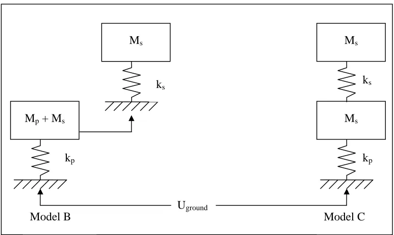
In the following section, we will discuss the main features associated with the coupling of a set of 2 linear oscillators. For the sake of simplicity, we shall work with a fixed mass ratio value of Rm=0.1, and frequency ratio Rf=1.25, i.e. “limit value” for SRP 3.7 and ASCE-4. Only seismic excitation will be considered, i.e. enforced acceleration at ground level, and response measured both on the primary and secondary structure.

Fig. 2 – Sequentially (mode B) vs directly (model C) coupled systems.

The mass [M] and stiffness [K]structural matrices for model C are as follows:

⎥

⎦

⎤

⎢

⎣

⎡

=

M

M

M

0

0

, and

⎥

⎦

⎤

⎢

⎣

⎡

−

−

+

=

K

K

K

K

K

K

For the sake of simplicity, we will assume Mp= 10 mass units while Ms=1 mass unit. Stiffness values Kp and Ks are cho-sen so as to have uncoupled natural frequencies fp and fs:

p p

p

f

M

K

=

(

2

π

)

K

=

(

2

π

f

)

M

Further simplifying can be obtained using a unitary value for fp i.e. fp = 1 cycle/unit time, so that fs=Rf=1.25 cycle/unit time. In the following, we will compare model “B” and model “C” results in terms of modal, harmonic, and transient dy-namic behavior, in order to appreciate the salient features of dydy-namic coupling.

Modal analysis:

A modal analysis run with model “B” and “C” yields the following results:

Modal frequency Model B Model C Diff [%]

Primary side 0.954 0.908 -5%

Secondary side 1.25 1.376 +10%

Table 1 – Modal frequencies for a set of 2 mechanical oscillators Rm=0.1 and Rf=1.25 obtained using “B” and “C” models

First of all, it should be noted that using this mass and frequency ratio, the frequency offset between the simplified and “best estimate” figures is exactly 10%. The discrepancies witnessed here are introduced by dynamic coupling that virtually:

• Increase the added mass effect of the primary mass created by the secondary mass,

• Increase the stiffness experienced by the secondary mass.

This somewhat counter-intuitive result asks for some clarification, since it will be foundation for the coming discussion. Basically, it could be felt that replacing the “rigid link” that exists between primary and secondary mass in model “B” by a more flexible one should somehow decouple the two masses and the frequency shift experienced by the primary mass should be reduced. Conversely, replacing the motionless – rigid- foundation seen by the secondary model B by a more movable one should introduce some flexibility into the system and the secondary mass should experience a downward shift in modal fre-quency.

This is where the concept of mechanical impedance is most helpful. For a given point-like system, it is defined as the ra-tio between input force and resulting mora-tion velocity.

M

+ M

M

M

M

k

k

k

k

Model B

Model C

pedance is therefore dominated by its imaginary part.

• Around natural frequency, oscillator response is at its maximum, and is in quadrature with the forcing function. Mechanical impedance is nearly purely real-valued, and positive, corresponding to a purely resistive condition.

• Above natural frequency, the oscillator response is mass dominated. Displacement is out-of-phase with loading. It is rapidly decreasing as the forcing frequency increases.

We shall now turn to our 2 DOFs system:

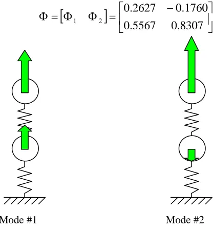
• For mode number 1 (dominated by primary structure), since fs>fp the mechanical impedance of the secondary structure is still stiffness dominated, so that secondary mass motion is in-phase with the primary motion, but its amplitude is much higher than that of the primary mass. As a consequence the kinetic energy added by the sec-ondary mass to the system is more than that strictly approportionned to the mass ratio, i.e. model B situation.

• For mode number 2 (dominated by secondary structure), since fp<fs the mechanical impedance of the primary structure is mass-dominated, so that the primary mass motion is out-of-phase with the secondary motion, and its amplitude is much lower than that of the secondary mass. Consequently, the strain energy stored in secondary stiffness is higher than if primary mass stood motionless. Modal frequency is therefore higher than that of the fixed-base condition, i.e, model B situation.

All this reasoning can be checked by inspecting the terms of the so-called “modal matrix” Φ, containing the system natu-ral modes shapes:

[

]

_⎥

⎦

⎤

⎢

⎣

⎡

−

=

Φ

Φ

=

Φ

8307

.

0

5567

.

0

1760

.

0

2627

.

0

2 1

Fig. 3 – Modes shapes of a set of 2 oscillators Rm=0.1 Rf=1.25

Before turning to a transient seismic analysis, the dynamic response of this system will be explored in more details using a harmonic (i.e. frequency sweep) seismic analysis.

Harmonic response analysis:

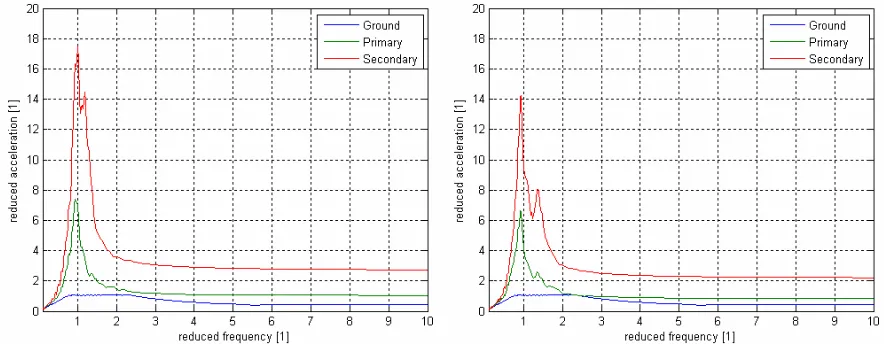
To allow for a deeper understanding of the structure seismic response, we shall compute the harmonic response of this 2 Oscillators system to a unitary acceleration signal enforced at base.

• Using model “B”: i.e. first compute acceleration on the primary mass, then enforce this acceleration at secon-dary mass foundation, or alternatively

• Using model “C”: compute the overall system response using a single, coupled dynamic model. A damping level of 4% was selected, corresponding to both reinforced concrete and welded steel structures. The results are as follows:

Fig. 4 – Harmonic responses of a set of 2 oscillators Rm=0.1 Rf=1.25 (model “B” – left hand side vs model “C” – right hand side)

It is quite obvious that not only have the “frequency gap” between oscillators grown significantly, but also the overall re-sponse level has decreased, most significantly in the amplified region, i.e. in the vicinity of the system natural frequencies. It should be noted, however, that coupling also introduced a small, secondary peak on the primary structure response that did not exist previously. It is also useful to manually derive the peak values for these two frequency response functions:

Model “B”:

• response for primary structure at fp: Hp(fp)=1/(2 ζ ) = 1/ (2x.04)= 12.5

• response for secondary structure at fp : Hs(fp)=Hp(fp)/(1-(fp/fs)²)=2.36x12.5=29.5

• response for primary structure at fs: Hp(fs)=1/(1-(fs/fp)²) = 1.37

• response for secondary structure at fs : Hs(fs)=Hp(fs)* 1/(2 ζ )=1.37*12.5=17.1

Model “C”:

• participation factors for modes #1 and #2 are respectively equal to Г1=3.184 and Г2=-0.930

• modal response for modes #1 and #2 : α1(f1)= Г1*(1/(2 ζ ))//(2π f2)²=1.22 and α2(f2)= Г2*(1/(2 ζ ))/(2π f2)²=0.155

• response for primary structure at f1: Hp(f1)= (α1(f1) Φ1p+ α2(f1) Φ2p)_{(2π f1)² = 10.4}

• response for secondary structure at f1: Hs(f1)= (α1(f1) Φ1s+ α2(f1) Φ2s)(2π f1)² = 22.1

• response for primary structure at f2: Hp(f2)= (α1(f2) Φ1p+ α2(f2) Φ2p)(2π f2)² = 2.1

• response for secondary structure at f1: Hs(f2)= (α1(f2) Φ1s+ α2(f2) Φ2s)(2π f2)² = 9.6

So far, a substantial reduction (the so-called “dynamic absorber” effect) has been witnessed, particularly on the peaks of the system frequency response functions.

However, although harmonic response analysis provides useful insight in that sense that it represents the structural re-sponse, this only corresponds to the “limit case” of very narrow band signals. Since seismic ground signals are basically broad-band signals, a measure of the total output power (in lieu of the peak amplitudes) would be a good indication of the overall response level to be expected.

This can be most easily obtained using the equivalent bandwidth of each mass, i.e. its total output power when subjected to an unlimited, white-noise type of excitation.

This quantity is given by the following formula:

∫

+∞

=

0 2

²

)

(

f

df

H

B

Numerically, for our 2DOFs system, we get the following figures:

Equivalent bandwidth Model B Model C Diff [%]

Primary mass 4.32 3.66 -15%

For checking purpose, we should run an analysis with both modelizations, and compare the response spectra obtained at each mass. The seismic ground motion is to be selected so as to be perfectly flat within the structure amplifying region, in order not to introduce any unwanted side-effect i.e., artificial peaks reduction due to a modal frequency sliding outside of the “plateau” region, for which the ground response spectrum amplitude is constant and equal to unity.

Fig. 5 – Response spectra of acceleration T-H of a set of 2 oscillators Rm=0.1 Rf=1.25 (model “B” – left hand side vs model “C” – right hand side)

The observed behavior is consistent with that obtained from the harmonic response analysis, i.e.:

• moderate reduction for the peak response of mode 1 (in-phase mode)

• significant reduction for the peak response of mode 2 (out-of-phase mode)

The reduction of peaks accelerations (ZPA) is about 20% for primary mass, and 33% for secondary mass, so that the es-timations provided by the equivalent bandwidth ratios prove to be rather reliable.

APPLICATION TO REACTOR BUILDING / REACTOR COOLANT SYSTEM SEISMIC ANALYSIS

We shall now turn to a “full scale”, structural analysis typical of Pressurized Water Reactor situations. Although the Reactor Buildings and the Reactor Coolant System are clearly complex, multi-modal structures, it is worth recognizing that relatively few modes are significant for a seismic analysis. To name a few:

• Reactor Building first two or three horizontal modes in each direction (mixed rocking / shear / bending),

• Reactor Coolant System “heavy” modes: in phase bending or translation of heaviest components (SG & RPV)

Although figures obviously vary for each design, it is worth keeping in mind that the RCS total mass is about 5-6% of the Interior Concrete Structure total mass. It should not be overlooked that for rock-like conditions, the basemat (representing about 45% of the ICS total mass) is motionless and consequently its mass counts for nothing. Therefore the mass ratio Rm is more in the 9-11% range, i.e. near the regulatory limit values. In order to somehow enhance the phenomena, the following situation will be used:

• Firstly, a rock-like soil condition is chosen so that only the Interior Structure bending modes come into play, and thus a small set of eigenmodes will be participating,

• Secondly, a 4-loops NSSS is selected, so there exists a neat “entire RCS” horizontal mode, for which SG and RPV move in-phase along the same line, thus with a participating mass about 50% the RCS total mass.

In such a situation, one would typically have to decide whether or not to couple structures having the following modal behav-ior:

Interior Structures Reactor Coolant System

• First order horizontal modes ~ 6/7 Hz (in phase translation of all levels).

• Second order horizontal modes ~14 / 15 Hz (upper levels out-of phase with lower levels)

• First vertical mode ~ 18 Hz.

• In phase SG bending ~ 6 Hz, 20% total mass

• Entire RCS horizontal ~ 10 / 12 Hz 50% total mass

• SG vertical ~ 14 Hz, 50% total mass

• RPV vertical ~ 27 Hz, 25% total mass

Table 3 –Typical modal behavior of ICS / RCS

Since only the modes having a frequency ratio near unity and acting predominantly along the same axis can significantly in-teract, the task of identifying potential effects of coupling is relatively straightforward. From this table, we can see that :

• Firstly: because of nearly matching frequencies, the RB first horizontal mode could be heavily coupled with SG in-phase bending. This should result in reductions, especially at elevated levels, where the first ICS mode dominates.

• Secondly, the “RCS entire translation” modal frequency being relatively remote from that of the ICS second hori-zontal modes, but its mass being quite significant, coupling effects should also be noticeable.

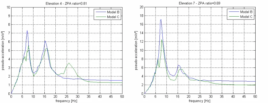
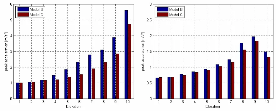
• Lastly, it can also be anticipated that the RCS vertical modes could significantly interact with the building response. The obtained behavior matches fairly well with that expected:

Fig. 6 – Response spectra of horizontal acceleration T-H for Model B and C. Left-hand side: RCS support level Right hand-side : SG upper supports level

The strong interaction between horizontal ICS and RCS modes around 6 Hz is evidenced by the fact that the first mode is “split” into two peaks of lesser amplitudes. There is also a reduction for the second order horizontal modes around 15 Hz, but the twin peaks patterns doesn’t show, since modal frequencies are not close enough.

Fig. 7 – Peak values of acceleration T-H for Model B and C. Left-hand side: horizontal axis Right hand-side : vertical axis

SUMMARY AND CONCLUSION

In this review we have shown that decoupling criteria are built so as to introduce shifts of less than 10% in modal fre-quencies. However, this doesn’t always ensure that the overall response level will be modified by less than 10% if coupled computations are used. It has been shown that when a set of oscillators are coupled, there exists a general trend toward re-sponse reduction, particularly for the supported structure. The conditions for a significant reduction in overall levels to exist have been identified. Extension to real, multi-modal cases have been done by conducting a typical case-study, in order to show how to explain and anticipate the effects of coupled computations.

NOMENCLATURE

αi = modal amplitude of mode i.

ζ = modal viscous damping ratio (fraction of critical damping) Гi = mode i participation factor (Гi = Φi M U)

Φi = mode i eigenvector

fp,s = primary (resp. secondary) structural uncoupled natural frequency

f1,2 = first (resp. second) structural coupled natural frequency

H = frequency response function (complex ratio between input and output motion) Rm = mass ratio, i.e. secondary mass divided by primary mass

Rf = frequency ratio, ratio of uncoupled natural frequencies

REFERENCES

[1] S.R.P. 3.7.2 “Seismic System Analysis” (1989)