A bayesian kernel for the prediction of protein-protein interactions

Abstract—Understanding proteins functions is a major goal in the post-genomic era. Proteins usually work in context of other proteins and rarely function alone. Therefore, it is highly relevant to study the interaction partners of a protein in order to understand its function. Machine learning techniques have been widely applied to predict protein-protein interactions. Kernel functions play an important role for a successful machine learning technique. Choosing the appropriate kernel function can lead to a better accuracy in a binary classifier such as the support vector machines. In this paper, we describe a Bayesian kernel for the support vector machine to predict protein-protein interactions. The use of Bayesian kernel can improve the classifier performance by incorporating the probability characteristic of the available experimental protein-protein interactions data that were compiled from different sources. In addition, the probabilistic output from the Bayesian kernel can assist biologists to conduct more research on the highly predicted interactions. The results show that the accuracy of the classifier has been improved using the Bayesian kernel compared to the standard SVM kernels. These results imply that protein-protein interaction can be predicted using Bayesian kernel with better accuracy compared to the standard SVM kernels.

Keywords—Bioinformatics, Protein-protein interactions, Bayesian Kernel, Support Vector Machines.

I. INTRODUCTION

HErecent studies of proteomics and molecular biology led

the researchers to recognize that protein-protein interactions (PPI) affect almost all processes in a cell [1], [2]. The prediction of protein–protein interaction is an important problem because it helps to understand the basis of cellular operations and other functions. It has been shown that proteins with similar functions are more likely to interact [2]. If the function of one protein is known then the function of its binding partners is likely to be related. This helps to understand the functional roles of unannotated proteins by knowing its interaction partners. Drug discovery is another

Hany Alashwal, is with the college of Pharmacy, University of Rhode Island, Kingston, RI 02881, USA (phone: 401-874-5368; fax: 401-874-2516; e-mail: [email protected]).

Safaai Deris, is with the Software Engineering Department at the Faculty of Computer Science and Information Systems, Universiti Teknologi Malaysia, 81310 Skudai, Johor, Malaysia, (e-mail: [email protected]).

Razib M. Othman is with the Software Engineering Department at the Faculty of Computer Science and Information Systems, Universiti Teknologi Malaysia, 81310 Skudai, Johor, Malaysia, (e-mail: [email protected]).

area where protein–protein interaction prediction plays an important role.

Therefore, understanding protein-protein interactions in a large scale is one of the important challenges of the post-genomic era. In this context, large-scale attempts have explored the complex network of protein interactions in the Saccharomyces cerevisiae [3] - [5]. It has been reported that even simple single-celled organisms such as yeast have about 6,000 proteins interact by at least three interactions per protein, i.e. a total of 20,000 interactions or more [6]. It is also estimated that, there may be nearly 100,000 interactions in the human body.

Since the number of proteins is in the thousands, the number of possible interacting pairs is in the millions, discovering actual interactions from these possible interactions using small-scale experiments become very labor-intensive and time-consuming. Hence, in this situation large-scale experiments are preferred. However, datasets obtained by large-scale, high-throughput methods for detecting protein–protein interactions typically suffer from a relatively high level of noise [7].

Therefore, several computational methods have been developed to predict protein-protein interactions which may lead to a better understanding of the functional relationships between proteins.

II. RELATEDWORKS

Several recent studies have investigated the applicability of Bayesian approaches for the prediction of protein-protein interactions. The Bayesian networks have been successfully applied to predict proteins that are in the same protein complex [8]. This means that their goal is to predict whether two proteins are in the same complex, not whether they necessarily had direct physical interaction. Having the problem of protein-protein interactions simplified to protein complexes prediction, the construction of gold standard data is feasible by taking the positives from Munich Information center for Protein Sequences (MIPS) catalog of known protein complexes and building the negatives from proteins that are known to be separated in different subcellular compartments. However, to apply Bayesian networks on predicting physical protein-protein interactions in genome-wide scale, the time complexity and negative examples unavailability are of concern.

A Bayesian Kernel for the Prediction of

Protein-Protein Interactions

Hany Alashwal, Safaai Deris and Razib M. Othman

T

In an attempt to resolve the issues in Bayesian networks approach to predict protein-protein interaction, [9] proposed combining decision trees and Bayesian networks. Their results show that Gene Ontology (GO) annotations can be a useful predictor for protein-protein interactions and that prediction performance can be improved by combining results from both decision trees and Bayesian networks. However, to get a higher quality and more complete interaction map, more types of data have to be combined, including gene expression, phenotype, and protein domains.

In another recent study a method based on the concept of Bayesian inference and implemented via the sum-product algorithm is applied for predicting domain-domain and protein-protein interactions by computing their probabilities conditioned on the measurement results [10]. The task of calculating these conditional probabilities are formulated as a functional marginalization problem, where the multivariates function to be marginalized naturally factors into simpler local functions. This framework enables the building of probabilistic domain-domain interactions to predict new potential protein-protein interactions based on that information. However, the Bayesian inference approach performance in real data is characterized by low specificity rate. The reason for this limitation of the Bayesian inference with sum-product algorithm, as mentioned by the author, is the higher sensitivity to assumed values of false positive rate (FPR), false negative rate (FNR), and a priori domain-domain interactions probability.

Although Bayesian networks have been applied successfully in a variety of applications, they are unsuitable representation for complex domains involving many entities that interact with each other [11].

In order to incorporate the advantages of Bayesian approach in predicting protein-protein interactions and to avoid its time complexity drawback, Bayesian kernel is introduced in [12]. In the following sections, a discussion on Bayesian approaches and kernel methods is presented.

III. BAYESIANAPPROACH

To understand Bayesian kernel and Bayesian related learning techniques, it is important to understand the Bayesian approach to probability and statistics. In this section, we present a brief introduction to the Bayesian approach to probability and Bayesian learning techniques.

A. Bayesian Probability

Bayesian probability is an interpretation of probability suggested by Bayesian theory, which holds that the concept of probability can be defined as the degree to which a person believes a proposition. Bayesian theory also suggests that Bayes’ theorem can be used as a rule to infer or update the degree of belief in light of new information.

In brief, the Bayesian probability of an event A is a person’s degree of belief in that event. Whereas a classical probability is a physical property of the world (e.g., the probability that a coin will land heads), a Bayesian probability is a property of

the person who assigns the probability (e.g., person’s degree of belief that the coin will land heads [13].

The Bayesians probability essentially considers conditional probabilities as more basic than joint probabilities. It is easy to define P(A|B) without reference to the joint probability

P(A,B). To see this, the joint and conditional probability formulas can be written as follows:

( , ) ( | ) ( ) ( | ) ( )

P A B P A B P B P B A P A (1)

It follows that:

( | ) ( ) ( | )

( )

P B A P A P A B

P B (2)

Equation (2) represents the Bayes’ Rule. It is common to think of Bayes rule in terms of updating our belief about a hypothesis A in the light of new evidence B. Specifically, our posterior belief P(A|B) is calculated by multiplying our prior belief P(A) by the likelihood P(B|A) that B will occur if A is true.

B. Bayesian Networks

Bayesian inference is a statistical inference in which evidence or observations are used to update or to newly infer the probability that a hypothesis may be true. One of the most common techniques to perform Bayesian inference is the Bayesian Networks.

The Bayesian network is a directed acyclic graph which represents independencies embodied in a given joint probability distribution over a set of variables. Nodes can represent any kind of variable such as measured parameters, latent variables or hypothesis. In the Bayesian network graph, nodes correspond to variables of interest and edges between two nodes correspond to a possible dependence between variables.

Over the last decade, the Bayesian network has become a popular representation for encoding uncertain expert knowledge in expert systems [14]. Recently, researchers started to develop methods for learning Bayesian networks from data. The techniques that have been developed are new and still evolving, but they have been shown to be remarkably effective for some data analysis problems (Niculescu and Mitchell, 2006).

The Bayesian Networks can be represented by a set of variables X { ,x₁",x₂}that encodes a set of conditional independence between these variables. A set P of local probability distributions associated with each variable should be defined. The conditional independence and the local probability define the joint probability distribution for X. The variable and its corresponding node in the network are denoted by

i

x and the parents of node x_iare denoted by pai.

Given these notations, the joint probability distribution for X

is given by:

1

( ) ( | )

n

i i

i

P x

–

P x pa (3)

The probabilities set by a Bayesian networks can be a Bayesian or physical. When prior knowledge is used alone, then the probabilities will be Bayesian. But when learning these networks from data, the probabilities will be physical.

IV. BAYESIANKERNELS

The Bayesian kernel exhibits some differences with respect to the standard kernels of SVM. Firstly, in the Bayesian kernel, the prior knowledge can be incorporated into the process of estimation. Secondly, in contrast to the standard kernels of SVM, which simply returns a binary decision, yes or no, a Bayesian kernel returns the probability, P y

1|x

, that an object x belongs to the class of interest indicated by the binary variable y. The probability result is more desirable than a simple binary decision as it provides additional information about the certainty of the prediction.

The Relevance Vector Machines (RVM) has been introduced by [15] which is a probabilistic sparse kernel method identical in functionality to the SVM. In RVM, a Bayesian approach to learning is adopted. The RVM does not suffer from significant limitations of the SVM. These limitations of the SVM are:

• Predictions are not probabilistic.

• It is necessary to estimate the error or margin trade-off parameter. This generally entails a cross-validation procedure, which is wasteful both of data and computation

However, the main disadvantage of RVM is in the complexity of the training phase [15]. For large datasets, the RVM makes training considerably slower than for the SVM. Given this fact, designing Bayesian kernel for the SVM would exhibit the advantages of the Bayesian approach and at the same time avoids the complexity problem of the RVM.

Recently, a Bayesian kernel for the prediction of neuron properties from binary gene profiles has been developed by [12]. They provided an analysis of the probabilistic model of the gene amplification process. This analysis yields a similarity measure between two strings of amplified genes that takes the asymmetry of the amplification process into account. This similarity measure was implemented in the form of Bayesian kernel.

This kernel was designed based on the probability of the expressed genes to be the same in both neurons. Given two strings

x

_iand

x

_jof amplified gene, the similarity between the strings is quantified as the probability for the expressed genes to be the same in both neurons and it is expressed as following:

_i, _j

_{i j} | _{i i}, _{j j}

k x x P Z Z X x X x (4)

Here,X refers to the random variables on

_{^ `}

0,1 Nstanding for the string of amplified genes (measurement), and Z the string of expressed genes (hidden truth). The value 1 stands for “expressed” or “amplified” while 0 stands for “non expressed” or “non amplified”. The only information available here is the value of X, and it is required to infer some property ofZ from the stochastic relation between X and Z. The value of Equation (4) can be evaluated with the Bayesian rule. It is given that

X

_i and

X

_j are independent, and that

Z

_i and

j

Z

are independent too. Also, according to amplification

model in [12], the

X

_il are conditionally independent. Then:

1

,

,

N

l l

i j l i j

l

k x x

_–

N

x

x

(5)

with

^ `0,1

, l | l l | l

l i i j j

c

a b P Z c X a P Z c X b

N



¦

(6)

The

N

_lcan be interpreted as a similarity measure between neurons based on the presence or absence of the l-th gene alone. It will take into account the high false negative rate and the absence of false positive.

V. BAYESIANKERNEL FOR PROTEIN-PROTEININTERACTIONS

PREDICTION

The implementation of a Bayesian kernel for protein-protein interactions prediction will facilitate incorporating the prior knowledge via the kernel function. The Bayesian learning is based on the Bayesian rule. In the following, uppercase letters will be used to represent variables and lowercase letters to represent realization. In predicting protein-protein interactions, each observation may be represented by a vector

Z

^

X

₁

,

!

,

X

_m

,

Y

`

,

where

^

1

,

,

m

`

X

X

!

X

is the m-dimensional input variable, and

Y is the output variable taking

_{^ `}

0,1 . Then dataset is represented by:

^

`

1 1 1 1

1 2 1

1 2

, ,

m n

n n n n

m

x x x y

D Z Z

x x x y

§ ·

¨ ¸

¨ ¸

¨ ¸

© ¹

"

! # # # # # "

(7)

The conditional probability of given can be represented as:

1 1

1 1

1 1

1, , ,

1| , ,

, ,

i i i i i

m j

i i i i i

m m i i i i

j m

P Y X x X x

P Y X x X x

P X x X x

" "

"

^ `

1 1

1 1

0,1

, , | 1 1

, , |

i i i i i i

m m

i i i i i i

m m

y

P X x X x Y P Y

P X x X x Y y P Y y

¦

"

" (8)

and

0 | 1, ,

1

1| 1, ,

i i i i i i

m m

P Y X " X P Y X " X (9)

where P Y

i yi

is the prior probability of

Y

itaking

value

y

iand the distribution for the conditional probability

1, , |

i i i

m

P X " X Y can be estimated from the dataset. Assuming that the input variables are independent for protein-protein interactions dataset, Equation (8) can be described as follows:

1| 1 1, ,

i i i i i

m m

P Y X x " X x

^ `

1 1

1 1

0,1

| 1 | 1 1

| |

i i i i i i i

m m

i i i i i i i

m m

y

P X x Y P X x Y P Y

P X x Y y P X x Y y P Y y

¦

"

" (10)

In a similar approach to [12] as described in Equations (5) and (6), we define a Bayesian kernel for protein-protein interactions prediction as:

1

,

,

m

i j i j

l l l l

k x

x

_–

N

x

x

(11)

with,

^ `0,1

,

|

|

i j i i i j j j

l l l l l l l

y

x x

P Y

y X

x P Y

y X

x

N



¦

(12)

The

N

_l can be interpreted as a similarity measure between protein pairs based on the l-th position of the feature vector. In this experiment we used the domain structure as the protein feature for the representation of the feature vector. For the prior and conditional probability of domains features to facilitate the protein-protein interactions we used the Appearance Probability (AP) matrix that was introduced in (16).

The domain combinations and the appearance frequency information of domain combinations are obtained from the interacting and non-interacting sets of protein pairs. The obtained information is stored in the form of a matrix called the Appearance Probability (AP) matrix. When there are n different proteins

^

p p

₁

,

₂

,

!

,

p

_n

`

in a given set of protein pairs and the union of domain combinations of proteins contains m different domain combinations,

^

d d₁, ₂,!,d_m

`

,

and then the

m

u

m

AP matrix is constructed. The element

AP

_ij in the matrix represents the appearance probability of domain combination

d d

_i

,

_j

!

in the given set of protein pairs. Then the conditional probability in Equation (12) can be obtained by:

i

1|

_li _li

AP

_il

P Y

X

x

(13)

VI. RESULTS AND DISCUSSION

In this section, the performance of the SVM classifier with the Bayesian kernel is discussed. For a detailed description of the dataset and features representation used in this experiment please refer to [17].

For constructing the positive interaction set, we represent an interaction pair by concatenating feature vectors of each proteins pair that are listed in the DIP-CORE as interacting proteins. Since we use domain feature we include only the proteins that have structure domains. The resulting positive set for domain feature contains 1879 protein pairs.

Constructing a negative interaction set using a random approach to construct the negative data set is an avoidable at this moment. Furthermore, for the purposes of comparing different kernel methods, the resulting inaccuracy will be approximately uniform with respect to each kernel method. For these reasons, the negative interaction set was constructed by generating random protein pairs. Then, all protein pairs that exist in DIP were eliminated. A negative interaction set was constructed containing the same number of protein pairs.

In our computational experiment, we employed the LIBSVM (version 2.5) software [18] and modified it to use the Bayesian kernel defined in this paper. The performance of the SVM with the Bayesian kernel is compared to the other four standard kernels described in Section 6.5.

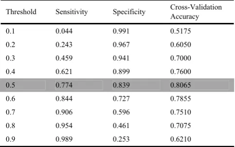
Table I shows the performance of the SVM with Bayesian kernel using domain feature with varied threshold. It shows that there is always a trade off between the sensitivity and specificity. The best cross-validation accuracy is achieved with threshold of 0.5. The specificity is higher than the sensitivity when choosing to have best cross-validation accuracy. This means that the Bayesian kernel can detect the non-interacting protein pairs with a reliable accuracy.

The performance of the Bayesian kernel compared to the other four standard kernels is presented in Table II. The Bayesian kernel has significantly improved the prediction accuracy compared to the linear and polynomial kernel. However, it has slightly improved the prediction accuracy compared to the RBF and sigmoid kernel. However, it is important to note the Bayesian kernel has the advantage of the probabilistic output over the RBF and sigmoid kernel. It help biologist to conduct further analysis on the predicted interacting proteins pairs with high probability.

Another aspect of performance measurement is the running time. From Table II, it is clear that the Bayesian kernel have achieved better performance in terms of computational running time compared to the RBF and Sigmoid kernels.

The ROC curve is also used to compare the performance of the Bayesian kernel against the standard kernel. Fig. 1 shows the ROC curve with ROC score for each kernel. The Bayesian kernel performs better than the standard kernels and has higher ROC score.

The distribution of the probabilistic output for the Bayesian kernel is shown in Fig. 2. The Bayesian kernel output a scalar value showing its belief in classification decision. Each protein pair that was predicted either interacting pair or non-interacting pair is assigned a likelihood of the predicted value. From Fig. 2, we can see that the number of protein pairs that have been predicted as interacting pairs with likelihood bigger than 89% is less than 100 pairs which is very small number compared to number interacting protein in the training dataset (1879). However, biologist can carry out experiments to validate the results for the protein pairs that were predicted as interacting pairs with high likelihood. It is time-consuming and costly to carry out experiments to validate the results of all predicted protein pairs.

VII. CONCLUSION

The Bayesian kernel was developed based on the Bayes’ Rule. The performance results of the Bayesian kernel outperformed most of the cited related work with ROC score of 0.8670. However, the comparison with some other works is not feasible due to the fact that different datasets were used. In addition, constructing negative set of non-interacting proteins is still the source of the varied reported accuracy. This is because, until now there is no experimentally confirmed non-interacting proteins dataset. Different cited work use different random method to generate non-interacting protein pairs. In conclusion, the Bayesian kernel provides a better performance as well as probabilistic output that could help biologist to carry out further analysis. In conclusion the result of this study suggests that protein-protein interactions can be predicted from domain structure with reliable accuracy. Consequently,

Fig. 1 The ROC curve for the Bayesian kernel and the standards kernel

Fig.2 The distribution of the probabilistic output for the Bayesian kernel

TABLE I

BAYESIANKERNEL PERFORMANCE WITH VARIED THRESHOLD

Threshold Sensitivity Specificity Cross-Validation Accuracy

0.1 0.044 0.991 0.5175

0.2 0.243 0.967 0.6050

0.3 0.459 0.941 0.7000

0.4 0.621 0.899 0.7600

0.5 0.774 0.839 0.8065

0.6 0.844 0.727 0.7855

0.7 0.906 0.596 0.7510

0.8 0.954 0.461 0.7075

0.9 0.989 0.253 0.6210

TABLE II

BAYESIANKERNEL PERFORMANCE COMPARED TO THE STANDARD KERNELS

Kernel Sensitivit

y Specificity Accuracy Running Time

Linear 0.726 0.764 0.768 14 Seconds

Polynomial 0.731 0.787 0.772 21 Seconds

RBF 0.742 0.811 0.793 32 Seconds

Sigmoid 0.751 0.805 0.791 30 Seconds

Bayesian 0.774 0.839 0.8065 12 Seconds

these results show the possibility of proceeding directly from the automated identification of a cell’s gene products to inference of the protein interaction pairs, facilitating protein function and cellular signaling pathway identification.

REFERENCES

[1] H. Lodish, A. Berk, L. Zipursky, P. Matsudaira, D. Baltimore, and J. Darnell, Molecular cell biology (4th edition). W.H. Freeman, New York, 2000.

[2] B. Alberts, A. Johnson, J. Lewis, M. Raff, K.Roberts, and P. Walter,

Molecular Biology of the Cell (4th edition). Garland Science, 2002. [3] T. Ito, K. Tashiro, S. Muta, R. Ozawa, T. Chiba, M. Nishizawa, K.

Yamamoto, S. Kuhara, and Y. Sakaki, “Toward a protein-protein interaction map of the budding yeast: a comprehensive system to examine two-hybrid interactions in all possible combinations between the yeast proteins,” Proc. Natl. Acad. Sci. USA. 97: 1143-1147, 2000. [4] P. Uetz, L. Giot, G. Cagney, T.A. Mansfield, R.S. Judson, J.R. Knight,

D. Lockshon, V. Narayan, M. Srinivasan, et al., “A Comprehensive analysis of protein-protein interactions in Saccharomyces cerevisiae,”

Nature403:623 627, 2000.

[5] J. R. Newman, E. Wolf, and P. S. Kim, “A computationally directed screen identifying interacting coiled coils from Saccharomyces cerevisiae,”Proc. Natl. Acad. Sci. U. S. A. 97, 13203–13208, 2000. [6] P. Uetz and C. S. Vollert, “Protein-Protein Interactions,” Encyclopedic

Reference of Genomics and Proteomics in Molecular Medicine

(ERGPMM), Springer Verlag, 2005.

[7] E. M. Phizicky and S. Fields, “Protein-protein interactions: Method for detection and analysis,” Microbiological Reviews, pp.94-123, 1995. [8] R. Jansen, H. Yu, D. Greenbaum, Y. Kluger, N.J. Krogan, S. Chung, A.

Emili, M. Snyder, J.F. Greenblatt, and M. Gerstein. “A Bayesian networks approach for predicting protein-protein interactions from genomic data.” Science. 302, pp:449-453, 2003.

[9] J. Yu, F. Fotouhi, and R.L. Finley. “Combining Bayesian Networks and Decision Trees to Predict Drosophila melanogaster Protein-Protein Interactions.”In the 21st International Conference on Data Engineering Workshops. April 5-8. Tokyo, Japan. 2005.

[10] M. Sikora, F. Morcos, D.J. Costello, and J.A. Izaguirre. “Bayesian Inference of Protein and Domain Interactions Using the Sum-Product Algorithm.” Proc. Information Theory and Applications Workshop, San Diego, Jan. 29, 2007.

[11] D. Koller. “Probabilistic Relational Models Source.” Lecture Notes in Computer Science. 1634: 3-13. 1999.

[12] F. Fleuret and W. Gerstner. “A Bayesian Kernel for the Prediction of Neuron Properties from Binary Gene Profiles.” Proceedings of the IEEE International Conference on Machine Learning and Applications. Special session Applications of Machine Learning in Medicine and Biology (ICMLA):129–134. 2005.

[13] D. Heckerman, D. Geiger and D.Chickering. “Learning Bayesian networks: The combination of knowledge and statistical data.” Machine Learning. 20:197-243. 1995.

[14] P. Larrañaga, M.Y. Gallego, B. Sierra, L. Urkola, and M.J. Michelena. “Bayesian networks, rule induction and logistic regression in the prediction of the survival of women suffering from breast cancer.”

Lecture Notes in Artificial Intelligence. 1323. E. Costa, A. Cardoso (eds.):303-308. Springer-Verlag. 1997.

[15] M. Tipping. “The relevance vector machine.” In Advances in Neural Information Processing Systems, 12:652-658. Cambridge MIT Press, 2000.

[16] D.S. Han, H.S. Kim, W.H. Jang, and S.D. Lee. “PreSPI: A Domain Combination Based Prediction System for Protein-Protein Interaction.”

Nucleic Acids Research. 32(21): 6312-6320. 2004.

[17] H. Alashwal, S. Deris, and R. M. Othman. “One-class support vector machines for protein-protein interactions prediction.” International Journal of Biomedical Sciences, 1(2):120–127, 2006.

[18] C. C. Chang and C. J. Lin, “LIBSVM : a library for support vector machines,” 2001. Software available at http://www.csie.ntu.edu.tw/~cjlin/libsvm.