Prediction of High-throughput Protein-Protein Interactions and Calmodulin Binding Using Short Linear Motifs

(1)

Scholarship at UWindsor

Electronic Theses and Dissertations Theses, Dissertations, and Major Papers

2016

Prediction of High-throughput Protein-Protein Interactions and

Calmodulin Binding Using Short Linear Motifs

Yixun Li

University of Windsor

Follow this and additional works at: https://scholar.uwindsor.ca/etd

Recommended Citation Recommended Citation

Li, Yixun, "Prediction of High-throughput Protein-Protein Interactions and Calmodulin Binding Using Short Linear Motifs" (2016). Electronic Theses and Dissertations. 5839.

https://scholar.uwindsor.ca/etd/5839

This online database contains the full-text of PhD dissertations and Masters’ theses of University of Windsor students from 1954 forward. These documents are made available for personal study and research purposes only, in accordance with the Canadian Copyright Act and the Creative Commons license—CC BY-NC-ND (Attribution, Non-Commercial, No Derivative Works). Under this license, works must always be attributed to the copyright holder (original author), cannot be used for any commercial purposes, and may not be altered. Any other use would require the permission of the copyright holder. Students may inquire about withdrawing their dissertation and/or thesis from this database. For additional inquiries, please contact the repository administrator via email

(2)

Interactions and Calmodulin Binding Using

Short Linear Motifs

By

Yixun Li

A Thesis

Submitted to the Faculty of Graduate Studies through the School of Computer Science in Partial Fulfillment of the Requirements for

the Degree of Master of Science at the University of Windsor

Windsor, Ontario, Canada

2016

c

(3)

Using Short Linear Motifs

by

Yixun Li

APPROVED BY:

S. Nkurunziza

Department of Mathematics and Statistics

A. Mukhopadhyay School of Computer Science

A. Ngom, Advisor School of Computer Science

L. Rueda, co-Advisor School of Computer Science

(4)

I hereby certify that I am the sole author of this thesis and that no part of this thesis has been published or submitted for publication.

I certify that, to the best of my knowledge, my thesis does not infringe upon anyones copyright nor violate any proprietary rights and that any ideas, techniques, quotations, or any other material from the work of other people included in my thesis, published or oth-erwise, are fully acknowledged in accordance with the standard referencing practices. Fur-thermore, to the extent that I have included copyrighted material that surpasses the bounds of fair dealing within the meaning of the Canada Copyright Act, I certify that I have ob-tained a written permission from the copyright owner(s) to include such material(s) in my thesis and have included copies of such copyright clearances to my appendix.

(5)

(6)

I would like to express my sincere appreciation to my supervisor Dr. Alioune Ngom and Dr. Luis Rueda for their constant guidance and encouragement during my whole Master’s period at the University of Windsor; without their valuable help, this thesis would not have been possible.

I would also like to express my appreciation to my thesis committee members Dr. Asish Mukhopadhyay, Dr. S´ev´erien Nkurunziza. Thank you all for your valuable guidance and suggestions to this thesis.

Meanwhile, I would like to thank Dr. Mina Maleki for all the help during my research process, including finding resources about Calmodulin Binding proteins and providing me very helpful guidance for the classification experiments.

(7)

DECLARATION OF ORIGINALITY III

ABSTRACT IV

AKNOWLEDGEMENTS V

LIST OF TABLES VIII

LIST OF FIGURES IX

1 Introduction 1

1.1 Protein-protein Interaction . . . 1

1.2 Calmodulin Binding Proteins . . . 2

1.3 Motifs . . . 3

1.3.1 Short Linear Motifs . . . 3

1.3.2 Tools for Finding Motifs . . . 4

1.4 Tools for score processing . . . 6

1.4.1 Python . . . 6

1.4.2 Matlab . . . 7

1.5 Machine Learning . . . 7

1.5.1 Tool for classification: WEKA . . . 7

1.5.2 Classification algorithms . . . 8

1.5.3 Feature selection . . . 10

1.5.4 Evaluation method . . . 11

1.6 Motivation of this Thesis . . . 12

2 Review of the Literature 14 2.1 Approaches for Prediction of PPIs . . . 14

2.1.1 Prediction of PPIs using information from simple condon pairs . . . 14

2.1.2 Prediction of PPIs using information from protein sequences . . . . 17

2.2 Prediction of Protein Interactions Using SLiMs . . . 21

2.2.1 Predict obligate and non-obligate protein interaction complexes us-ing SLiMs . . . 21

2.3 Inspiration from the Previous Works . . . 25

3 Materials and Methods 26 3.1 Datasets . . . 26

3.1.1 Datasets for prediction of PPIs . . . 26

3.1.2 Datasets for prediction of CaM-binding proteins . . . 28

3.2 SLiMs Finding Approaches . . . 28

3.3 Scoring the Sites . . . 29

(8)

3.3.4 Scoring method variance 4: Counting sites withIˆformula /

count-ing of sites . . . 33

3.3.5 Scoring method 5: Sliding Window Scoring method . . . 33

3.4 Score Processing . . . 34

3.4.1 Score processing for prediction of PPIs . . . 36

3.4.2 Score processing for CaM-binding proteins . . . 37

3.5 Machine Learning Method Using for Classification . . . 37

4 Results 39 4.1 Results . . . 39

4.1.1 Classification results of prediction of PPIs . . . 39

4.1.2 Grid search for SVM-polynomial (prediction of PPIs) . . . 42

4.1.3 Classification results of prediction of CaM-binding proteins . . . . 42

4.1.4 Grid search for SVM-polynomial (prediction of CaM-binding pro-teins) . . . 47

4.2 Comparison . . . 49

4.2.1 Comparison between results of prediction of PPIs . . . 49

4.2.2 Comparison between results of prediction of CaM-binding proteins results . . . 49

4.2.3 Classification VS Classification + FS . . . 51

5 Conclusion and Future Work 54 5.1 Contributions . . . 54

5.2 Future Work . . . 55

References 56

(9)

3.3.1 Position-specific probability matrix of SLiM No.29. . . 30

4.1.1 Prediction of PPIs classification results for the score matrices with SLiMs obtained from the CM approach. . . 40 4.1.2 Accuracies of prediction of PPIs classification for the score matrices with

SLiMs obtained from the SM approach. . . 41 4.1.3 Accuracies (%) of prediction of PPIs using SVM-Polynomial (C = 1, 10,

100, 1000, gamma = 0.01, 0.1, 0, 1, 10, 100, 1000) with SLiMs obtained from SM. . . 43 4.1.4 Accuracies (%) of prediction of PPIs using SVM-Polynomial (C = 1, 10,

100, 1000, gamma = 0.01, 0.1, 0, 1, 10, 100, 1000) with SLiMs obtained from CM. . . 44 4.1.5 Prediction of CaM-binding proteins classification results for the score

ma-trices with SLiMs obtained from SM. . . 45

4.1.6 Prediction of CaM-binding proteins classification results for the score ma-trices with SLiMs obtained from CM. . . 46 4.1.7 Accuracies (%) of prediction of CaM-binding proteins using SVM-Polynomial

(C = 1, 10, 100, 1000, gamma = 0.01, 0.1, 0, 1, 10, 100, 1000) with SLiMs obtained from SM. . . 47 4.1.8 Accuracies (%) of prediction of CaM-binding proteins using SVM-Polynomial

(10)

1.2.1 Structure of CaM (green) interacting with its binding domain from

cal-cineurin (blue). . . 2

1.3.1 An amino-acids motif pattern. . . 3

1.3.2 The MEME Suite. Figure obtained from meme-suite.org. . . 5

1.5.1 WEKA software logo. . . 8

1.5.2 Optimal Separating Hyperplane [15]. . . 9

2.1.1 The results of classifying the original dataset using 1NN, SVM-RBF (Cost = 10 and Gamma = 5000), and Random Forest classifiers. . . 19

2.1.2 Using 1NN, SVM-RBF (Cost = 10 and Gamma = 5000), and Random For-est to classify the dataset obtained after applying feature selection. . . 19

2.1.3 Results of using SVM-RBF classifier (with Gamma fixed to 5000) based on accuracy on both original and selected feature datasets. . . 20

2.1.4 Results of using SVM-RBF classifier (Cost fixed to 10) based on accuracy on both original and selected feature detasets. . . 20

2.1.5 ROC curve for SVM-RBF (Gamma = 0.01, 0.1, 1, 10, 100, 1000, 5000, 10000, 20000, 100000 and Cost = 10). The blue star represents the best result, SVM-RBF (Gamma = 5000 and Cost = 10), with Area under ROC = 0.9165. . . 21

3.0.1 Diagram of the proposed model. . . 27

3.3.1 SLiM No.29 found in the CM dataset. . . 29

3.3.2 Example of obtaining scores using method variance 1 (Counting SLiMs). . 31

3.3.3 Example of obtaining scores using method variance 2 (Counting SLiMs withIformula). . . 32

(11)

teins. . . 36

4.2.1 Accuracies for prediction of PPIs for matrices with SLiMs obtained from CM. . . 50 4.2.2 Accuracies for prediction of PPIs for matrices with SLiMs obtained from

SM. . . 50 4.2.3 Accuracies for prediction of CaM-binding for matrices with SLiMs

ob-tained from CM. . . 51 4.2.4 Accuracies for prediction of CaM-binding for matrices with SLiMs

ob-tained from SM. . . 52 4.2.5 Comparison of prediction of CaM-binding proteins accuracies between

classification results by 1-NN for matrixes with SLiMs obtained from SM and matrixes with SLiMs obtained from CM. . . 52 4.2.6 Comparison of accuracies of classification results on PPIs by 1-NN (left)

and Random Forest (right) for original matrices obtained from SM and CM, with the results for matrices after feature selection. . . 53 4.2.7 Comparison of accuracies of classification results on CaM-binding proteins

(12)

Introduction

1.1 Protein-protein Interaction

Comprehensive analysis of protein-protein interactions(PPIs) has been regarded as very

significant for the understanding of underlying mechanisms involved in cellular processes [25]. PPIs are crucial for all biological processes [36]. While many proteins perform their functions when they interact with other proteins, understanding and studying PPIs is very important in almost all biological processes taking place in the cell, and help predict the function of unknown proteins [2].

PPIs networks provide a valuable framework for a better understanding of the func-tional organization of the proteome [36], and summarize large amounts of protein-protein interaction data, both from individual, small-scale experiments and from automated high-throughput screens [8]. Therefore, compiling PPI networks may provide new insights into protein function [36].

Common high-throughput experimental techniques for predicting PPIs such as Yeast

(13)

1.2 Calmodulin Binding Proteins

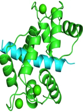
Calmodulin (CaM) is a calcium-binding protein that is a major transducer of calcium sig-naling [37]. It has no enzymatic activity on its own but rather acts by binding to and altering the activity on a panel of cellular protein targets. Its targets are structurally and function-ally diverse and participate in a wide range of physiological functions including immune response, muscle contraction and memory formation.

Figure 1.2.1 is a typical of calcium-dependent protein interaction, where the two halves of CaM bind to opposite sides of the target peptide (the four calcium molecules are green spheres). Identifying CaM target proteins and CaM sites is an important and ongoing re-search problem because of the great diversity of conformations it uses in its target interac-tions. This diversity cannot be captured by a single amino acid sequence motif, but instead CaM-binding sites are commonly divided into four or more motif classes with different sequence characteristics [43]. Current algorithms struggle to identify novel CaM-binding proteins.

(14)

1.3 Motifs

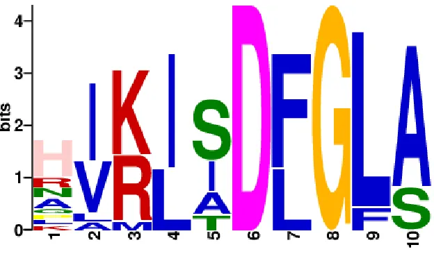
A motif is a sequence pattern of nucleotides in a DNA sequence or amino acids in a protein [42]. Motifs are patterns widespread over a group of proteins that are related by function or may have other biological features in common. Given a set of sequences, motifs are common subsequences, which appear the most among these sequences. Usually, each motif contains a sequence pattern of 3-20 amino acids [29].

FIGURE 1.3.1: An amino-acids motif pattern.

1.3.1 Short Linear Motifs

(15)

1.3.2 Tools for Finding Motifs

Motifs may be indistinguishable from random artifacts, therefore, discovering biological motifs in a set of sequences is a difficult task [6], and hence several approaches have been

proposed for improving motif discovery [6], such as usingauxiliary data, PSP approach

andGibbs Sampling.

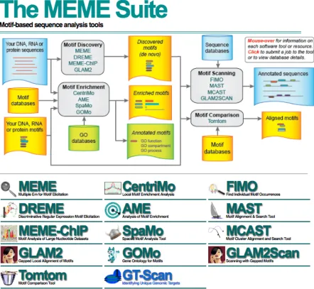
From different accessible SLiM discovering tools such as SLiMFinder [12], SLiM-Search [13], Minimotif Miner (MnM) [33], and MEME (Multiple EM for Motif Eluci-dation) [4], MEME can discover SLiMs through an unsupervised approach and turns out to be a very efficient and successful algorithm for discovering new SLiMs with different number of occurrences in a set of protein sequences. It discovers motifs by optimizing the statistical parameters of the model using the Expectation Maximization (EM) algorithm, and a statistical sequence model to determine the positions and the width of the motif sites in the sequences [6].

MEME provides both a Web server online and a stand-alone application that can be dowloaded and installed locally on Unix or Linux platforms. The MEME Suite Web server provides a unified portal for online discovery and analysis of sequence motifs representing features such as DNA binding sites and protein interaction domains. The popular MEME motif discovery algorithm is now complemented by the GLAM2 algorithm which allows discovery of motifs containing gaps. Three sequence scanning algorithms MAST, FIMO and GLAM2SCAN allow scanning numerous DNA and protein sequence databases for mo-tifs discovered by MEME and GLAM2 [3]. Figure 1.3.2 shows the Motif-based sequence analysis tools in the MEME Suite Website.

(16)

(17)

1.4 Tools for score processing

After we obtained the SLiMs from the protein datasets, we applied score processing for obtaining the score matrices for experiments. For processing the scores and the matrices, we use Python and Matlab for programming and matrix operations.

1.4.1 Python

Python is a popular programming language for scientific computing. It provide state-of-the-art implementations of many well known machine learning algorithms, and maintains an easy-to-use interface. Therefore, the need grows for statistical data analysis by non-specialists in the software and Web industries, as well as in fields outside of computer-science, such as biology or physics [26].

There are plenty of data analysis libraries and tools for Computational Biology writ-ten in Python, which can be downloaded for free from http://www.biopython.org, such as Biopython [11]. Biopython includes modules for reading and writing different sequence file formats and multiple sequence alignments, dealing with 3D macro molecular struc-tures, interacting with common tools such as BLAST, ClustalW and EMBOSS, accessing key online databases, as well as providing numerical methods for statistical learning [11]

(18)

1.4.2 Matlab

Matlab is a data analysis and visualization tool that has been designed with support for matrices and matrix operations. Matlab has excellent graphics capabilities, and its own powerful programming language. One of the reasons that Matlab has become such an important tool is through the use of sets of Matlab programs designed to support a particular task [22].

In this thesis, we use Matlab to devide the elements in one matrix by the elements in another matrix, where that elements are in the same position in their own matrix.

1.5 Machine Learning

Learning processes include the acquisition of new declarative knowledge, the develop-ment of motor and cognitive skills through instruction or practice, the organization of new knowledge into general, effective representations, and the discovery of new facts and the-ories through observation and experimentation [9]. As one of the most challenging goal in artificial intelligence, researchers have been striving to implant such capabilities in com-puters and make the machines learn new knowledge. This field is called Machine Leaning (ML).

1.5.1 Tool for classification: WEKA

Waikato Environment for Knowledge Analysis (Weka) is a collection of ML algorithms for data mining tasks. The algorithms can either be applied directly to a dataset or called from other Java programs [17].

(19)

to (a) assist users in extracting useful information from data and (b) enable them to easily identify a suitable algorithm for generating an accurate predictive model from it [14].

Weka is a flightless bird with an inquisitive nature, it is found only on the islands of New Zealand. The name is pronounced like this, and the bird sounds like the one shown in Figure 1.5.1, which shows the logo of the Weka software.

FIGURE 1.5.1: WEKA software logo.

1.5.2 Classification algorithms

Weka provides many classification methods such as BayesNet, NaiveBayes, LibSVM with linear/polynomial/radial basis function (RBF) kernel, RBFNetwork, Multilayer Perceptron,

k-Nearest Neighbor (kNN), Random Forest and Decision Tree, etc. In this thesis, we used

different classifiers: LibSVM + Polynomial, LibSVM + RBF, Random Forest, kNN, Deci-sion Tree and Multilayer Perceptron.

LibSVM is a library for Support Vector Machines (SVM) [10]. It is a powerful, state-of the art algorithm that can guarantee the lowest true error due to increasing the generalization capabilities [34]. LibSVM + linear was considered for our classification, as shown in Figure 1.5.2. Here, there are many possible linear classifiers that can separate the data, but there is only one that maximizes the margin (maximizes the distance between it and the nearest data point of each class). This linear classifier is termed the optimal separating hyperplane. Intuitively, we would expect this boundary to generalise well as opposed to other possible boundaries [15].

(20)

FIGURE 1.5.2: Optimal Separating Hyperplane [15].

non-linear models [41]. The RBF kernel is also commomly used in classifing non-linear models.

In SVM + Polynomial or RBF kernel, the gamma parameter defines how far the influ-ence of a single training example reaches, with low values meaning far and high values meaning close. The gamma parameters can be seen as the inverse of the radius of influence of samples selected by the model as support vectors. The C parameter trades off misclassi-fication of training examples against simplicity of the decision surface. A low C makes the decision surface smooth, while a high C aims at classifying all training examples correctly by giving the model freedom to select more samples as support vectors. In order to find the best parameters when using SVM classifier, we implied grid search with different C and gamma.

(21)

K-nearest-neighbor (kNN) is one of the most fundamental and simple classification methods and should be one of the first choices for a classification study when there is little or no prior knowledge about the distribution of the data. kNN was developed from the need to perform discriminant analysis when reliable parametric estimates of probability densities are unknown or difficult to determine [27].

Decision tree (DT) classifier is one of the possible approaches to multistage decision making. It is a way of representing a series of rules that lead to a class or value [34]. The basic idea involved in any multistage approach is to break up a complex decision into a union of several simpler decisions, hoping that the final solution obtained in this way would resemble the intended desired solution [31].

A multilayer perceptron (MLP) is a feedforward artificial neural network model that maps sets of input data onto a set of appropriate outputs. An MLP consists of multiple lay-ers of nodes in a directed graph, with each layer fully connected to the next one. Except for the input nodes, each node is a neuron (or processing element) with a nonlinear activation function. MLP utilizes a supervised learning technique called backpropagation for training the network. MLP is a modification of the standard linear perceptron and can distinguish data that are not linearly separable [40].

1.5.3 Feature selection

During the last decade, the motivation for applying feature selection (FS) techniques in bioinformatics has shifted from being an illustrative example to becoming a real prereq-uisite for model building. In particular, the high dimensional nature of many modelling tasks in bioinformatics, going from sequence analysis over microarray analysis to spectral analyses and literature mining has given rise to a wealth of FS techniques being presented in the field [30].

(22)

approach tailored to a specific classification algorithm [30]. In this thesis, we applied the wrapper approach with RF for FS followed by classification using different algorithms.

1.5.4 Evaluation method

The K-fold cross validation refers to testing procedure where the dataset is randomly

di-vided intoK disjoint blocks of objects. Then the data mining algorithm is trained usingk

- 1 blocks and the remaining blocks is used to test the performance of the algorithm. This

process is repeatedktimes. At the end, the recorded measures are averaged. It is common

to choosek=10 or any other size depending on the size of the original dataset [34]. In this

thesis, since the datasets are all not very large, we chosek=3 for evaluation.

We used the following performance measures: Accuracy,RecallandMatthews

correla-tion coefficient(MCC) in order to assess the predictive capability of our approach, because the the accuracy of random classifiers is 50% for balanced distributions [32] and a co-efficient of +1 represents a perfect prediction, 0 no better than random prediction and 1 indicates total disagreement between prediction and observation [39].

Accuracy = T P +T N

T P +F P +T N+F N (1.5.1)

Recall= T P

T P +F N (1.5.2)

M CC = √ T P ×T N −F P ×F N

(T P +F N)(T P +F P)(T N +F P)(T N+F N) (1.5.3)

(23)

1.6 Motivation of this Thesis

Prediction of protein-protein interaction (PPI) is a difficult and important problem in biol-ogy. Although high throughput technologies have made remarkable progress, the predic-tions are often inaccurate and include high rates of both false positives and false negatives. Meanwhile, prediction of Calmodulin-binding (CaM-binding) proteins plays a very impor-tant role in the fields of biology and biochemistry, because Calmodulin binds and regulates a multitude of protein targets affecting different cellular processes.

Short-linear motifs (SLiMs) in protein sequences have being effectively used as fea-tures for predicting and analyzing obligate protein interactions, several computational ap-proaches have been used for prediction of high-throughput PPIs, though their properties have not been used in the prediction of CaM-binding proteins, and none of them has ex-ploited the power of SLiMs. In this thesis, we propose five new methods for prediction of PPIs and CaM-binding proteins based on counting scores of SLiMs between pairs of protein sequences with specific scoring functions.

The extracted features are new SLiMs derived from MEME. Two different approaches have been used to discover new motifs using MEME: (a) find SLiMs from each of the pos-itive and negative datasets separately (SM) and (b) find SLiMs from the combined pospos-itive and negative datasets (CM).

As for prediction of PPIs, given two initial datasets of PPI pairs and non-PPI pairs, we first pre-processed the datasets into new smaller datasets as 50 PPI pairs and 38 non-PPI pairs for obtaining the SLiMs using MEME. We have used MEME to obtain 50 motifs for each of the positive and negative datasets, separately, obtaining a set of 100 motifs (the SM approach). Similarly, we generated 50 motifs from the combined negative and positive datasets (the CM approach).

(24)

Predictions of CaM-binding proteins have been performed in the Waikato Environment for Knowledge Analysis (WEKA) using k nearest neighbor (k-NN), Support support vector machine (SVM), random forest (RF), decision tree (DT) and Multilayer Perceptron (MP) classifiers, on a 3-fold cross-validation setup. Moreover, the wrapper criterion with Ran-dom Forest for feature selection (FS) has been applied followed by classification using different algorithms mentioned above.

Our method shows itself to be very promising and demonstrates that information con-tained in SLiMs is highly relevant for accurate prediction of PPIs and CaM-binding pro-teins. In addition to efficient prediction, individual SLiMs may bring extra information on meaningful patterns linked to specific roles in protein function.

(25)

Review of the Literature

Recent studies have focused on the approaches of prediction of PPIs, the discovery of new SLiMs, and the prediction of protein interactions using SLiMs. In this chapter, we review the previous research and publications on prediction of Protein-protein interactions and research on Short Linear Motifs.

2.1 Approaches for Prediction of PPIs

In this section, we review two papers related to prediction of protein interactions using protein sequence informations. The first paper proposes a codon pair usage-based PPI pre-diction method. The second paper proposes a new method based on animo acid defferences between pairs of protein sequences.

2.1.1 Prediction of PPIs using information from simple condon pairs

The authors of [45] analyze the relatiionship between codon pair usage and PPIs in yeast, and show that codon pair usage of interacting protein pairs deffers significantly from ran-domly expected. This motivates the development of a novel approach for predicting PPIs, CCPPI, with codon pair frequency defference as input to a SVM classifier. The results show that CCPPI performs better than other sequence-based encoding schemes.

Previous work and shortcomings by others referred to by the authors

(26)

mass spectrometry, miniatures of the interactomes of a few model organisms. However, the authors note that the experimental methods mentioned above are relatively expensive and labor intensive and suffering from insufficient coverage.

The new idea that the authors proposed

The authors proposed a codon pair usage-based PPI prediction method termed as CCPPI (Codon Combination-based Protein-Protein Interaction predictor) under the Support Vector Machine (SVM) framework. Their analyses show that codon pair usage of interacting protein pairs is significantly different from that of random protein pairs.

Materials and methods

They downloaded protein sequences and the corresponding coding sequences of yeast from the SGD database. They used three kinds of combined datasets of 4156 DIP positives and equal number of non-interacting protein pairs. The first kind of datsets that contains ran-domly selected non-interacting protein pairs as negatives are termed as “DIP + Random”. The second kind (“DIP + RSS Negative”) contains “RSS Negative” without known similar functions or subcellular localizations. The “RSS Negative” datasets were randomly se-lected protein pairs whose RSS (Biological Process) and RSS (Cellular Component) were less than 0.4. With respect to the third kind of datasets (“DIP + Homogeneous”), the nega-tives were generated by randomly rewiring the DIP posinega-tives.

They calculated the difference in a feature between a pair of proteins in specific scoring functions. They compared two previously published encoding schemes with their encoding schemes, CT encoding and AC encoding. They used the two encoding schemes to concate-nate feature vectors for a pair of proteins instead of calculating the differences between them.

(27)

CT encoding and AC encoding) perform better with C= 10than the default C. They use the following four perfomance measures for evaluating the results: accracy, precision, sen-sitivity and MCC. The definition of precision and sensen-sitivity are:

precision= T P

T P +F P (2.1.1)

sensitivity = T P

T P +F N (2.1.2)

Results and discussion

The authors claim to have compared codon pair frequency differences between 4,380 inter-acting protein pairs from the DIP database and randomly selected protein pairs, which are

19-fold larger than the former. In total, there are61×61 = 3721codon pairs under

inves-tigation. Compared with randomly selected protein pairs, 1551 out of 3721 codon pairs in the interacting protein pairs were observed to have significantly similar frequencies. At the same significance level, the frequencies of 619 codon pairs in interacting protein pairs tend to be dissimilar. Moreover, there is a considerable fraction (41.7%) of codon pairs that do not have any significant difference. In contrast, 57 out of 61 codons in the interacting pro-tein pairs show similar frequencies, which is consistent with previous observations based on a different dataset. They also claim that a predictor based on codon pair frequency dif-ferences may perform better in distinguishing interacting protein pairs from random protein pairs.

(28)

Their results indicate that the developed codon pair based method CCPPI is capable of predicting protein-protein interactions, with a favorable or at least competitive performance in comparing with several well-known sequence-based encoding schemes.

2.1.2 Prediction of PPIs using information from protein sequences

[21] describes our previous research related to prediction of PPIs based on amino acid differences between pairs of protein sequences. Our finding suggests that amino acid dif-ferences of interacting protein pairs are relevant to the prediction of PPIs and hence provide important imformation on sequence-based encoding schemes.

We state that the methods only using the information of protein sequences are more uni-versal than those that depend on some additional information or predictions about the pro-teins. Paper [16] achieved acceptable performance on the yeast dataset using AC encoding of physicochemical features derived from spaced amino acid pairs. Paper [35] proposed a CT encoding scheme based on the calculation of tri-peptide frequencies, and it was shown to achieve good results in the human PPI dataset. However, though several sequence-based methods have shown that the information of amino acid sequences alone may be sufficient to identify novel PPIs, the highest prediction accuracy of these methods is only 80%. The information of the interactions which occurs in the discontinuous amino acids segments in the sequence may be able to further improve the prediction ability of the existing sequence-based methods.

(29)

4,000 negative pairs from the Protein Data Bank (PDB) in the Negatome Database. We downloaded the protein sequences from Uniprot.

After obtaining the positive and negative protein sequences datasets we calculated the difference of the counting of different amino acids between each positive pair and each negative pair of proteins, and used the difference of each amino acid as the features for each pair of proteins.

Experiments and analysis

We applied Naive Bayes, kNN, DT, RF and SVM with different kernels (Linear, Poly-nomial and RBF) classifiers on our datasets using WEKA. 10-fold cross-validation is the method we used for validating all the classifiers. We used the following performance mea-sures in order to assess the predictive capability of our approach: accuracy, recall, FP rate, precision, F-measure and MCC.

We used the wrapper approach with mRmR (Minimum Redundancy and Maximum Relevance) which is available in WEKA. Random Forest was used within this wrapper for evaluating the accuracy of a feature subset.

Results that the authors claim to have achieved

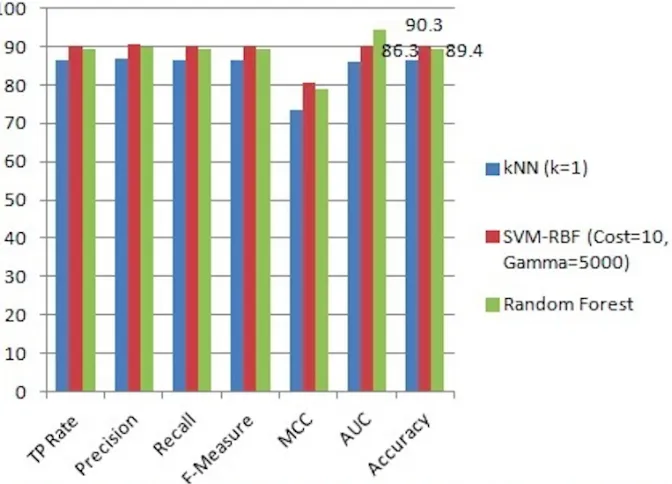
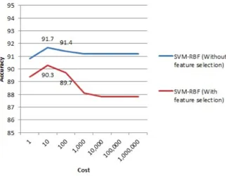
The accuracy results of the classifiers on the original full dataset and on the reduced dataset (after FS) are, respectively, 87.2% and 86.3% for kNN, 89.3% and 89.4% for Random Forest, and 91.7% and 90.3% for SVM-RBF (see Figures 2.1.1, 2.1.2, 2.1.3, and 2.1.4). The ROC curve for SVM-RBF is shown in Figures 2.1.5.

(30)

FIGURE 2.1.1: The results of classifying the original dataset using 1NN, SVM-RBF (Cost = 10 and Gamma = 5000), and Random Forest classifiers.

(31)

FIGURE 2.1.3: Results of using SVM-RBF classifier (with Gamma fixed to 5000) based on accuracy on both original and selected feature datasets.

(32)

FIGURE 2.1.5: ROC curve for SVM-RBF (Gamma = 0.01, 0.1, 1, 10, 100, 1000, 5000, 10000, 20000, 100000 and Cost = 10). The blue star represents the best result, SVM-RBF (Gamma = 5000 and Cost = 10), with Area under ROC = 0.9165.

2.2 Prediction of Protein Interactions Using SLiMs

In this section, we review a papers related to prediction of protein interactions using SLiMs. The paper has proposed a model that uses SLiMs as properties to predict obligate and non-obligate protein interaction complexes.

2.2.1 Predict obligate and non-obligate protein interaction complexes

using SLiMs

(33)

cross-dataset validation show that the information contained in the training sequences is crucial for prediction and determination of stability in PPIs.

The authors state that characterizing the properties of protein interaction types can be done by studying their sequence or structural information. The most effective approaches for prediction of PPIs use mainly structural information of protein complexes to calculate the feature values, and the PDB is the main source of the molecular structures of protein com-plexes.

However, models based on structural information from the PDB are not perfect yet and are time comsuming. In addition, the small number of proteins and their interactions from a small number of structures in PDB are very small compared to the number of possible pro-tein interactions available in high-throughput propro-tein and PPIs databases such as UniProt. Moreover, models based on protein structures are limited to availability of structural infor-mation. Overall, the authors gained the motivation of a model that can replace the use of structural properties.

The new idea which the authors invented

In that paper, the authors proposed a model that uses SLiMs as properties to predict

ob-ligate and non-obob-ligate protein complexes. The model uses k-NN, linear dimensionality

reduction (LDR) and SVM as the classifiers to predict these types. Their prediction results for two well-known datasets show prediction accuracy of more than 99%, which implies an increase of at least 7% from previous approaches, even beter than the state-of-art structure-based methods and using only sequence information.

(34)

obligate and 212 non-obligate complexes.

The authors chose MEME to find independent sets of SLiMs for the two datasets. They optimized the parameters of MEME to find 1,000 SLiMs in both the ZH and MW datasets. They set the length of the SLiMs to 3-10 and 2-7, the minimum number of sites to 8 and the maximun number of sites to 200. Based on the two length ranges of the SLiMs and the two datasets, four SLiM sets were compiled.

The authors indicate that for each complex in the dataset, its sequences are divided into

overlappingl-mer, which are the sites of motifs in the training set. Given a sequenceXof

lengthL, let us consider anl-mer ain the sequence, wherel is the length of each SLiM.

The scoring function they used for processing the scores of the motifs is shown in Formula 2.2.1:

I(a|X) = − l

X

i=1

P(ai)×log(P(ai)) (2.2.1)

where X is the profile sequence, P(ai) is the probability (of the ith residue of a) from

that profile. Since P(ai) ≤ 1,

Pl

i=1P(ai)is very small for large sites, -log gives a more

meaningful measure.

Equation (2.2.1) implies that that larger the site is, the larger the information content is. Thus, in that paper, they also divide the total information content by the length of the site,

lin order to erase the effect. Then the information content of a siteaof lengthl is defined

as:

ˆ

I(a|X) =−1

l ×

l

X

i=1

P(ai)×log(P(ai)) (2.2.2)

Since log(1) = 0, for anyP(ai)=1, a small threshold is subtracted from P(ai)as

(35)

logP(ai) =       

log(0.99) ifP(ai) = 1

log(P(ai)) otherwise

(2.2.3)

Experiments and analysis

They used two validation approaches for classification. (1) Leave-one-out validation with

ak-NN classifier, (2) a cross-dataset validation for testing the accuracy and significance of

the newly proposed features. They also chose SVM and LDR for cross-dataset validation classification because the power of generalization of the scheme in prediction of new com-plexes is provided by SVM and LDR. They used LibSVM with a linear kernel with default parameters for SVM.

Results that the authors claim to have achieved

As for the results of leave-one-out validation with k-NN, the highest accuracy is 98.54%

fork= 35 and the lowest is 95.62% fork = 5 whenl= 10. This scheme yields the highest

accuracy of 99.27% whenl= 9, 7, 6, 5. For the ZH dataset, the highest accuracy is 99.27%

for different values oflandk. Forl= 7, and all the values ofk, the accuracy is 99.27%. As

for the results of cross-dataset validation, the scheme yields the highest accuracy of 97.81%

and 99.27% forl= 5,4 respectively using SVM and different LDR for the ZH dataset with

the MW SLiMs for training. As in [46], they predicted obligate and non-obligate complexes with 88.32% accuracy.

(36)

2.3 Inspiration from the Previous Works

From the first paper of prediction of PPIs using simple codon pairs, we were inspired by the idea of prediction of PPIs using information in the protein sequences, and thus we experimented predicting PPIs using the difference of single amino acids between pairs of proteins. As a result, we not just focus on single amino acids, as we considered 1-gram. We have the idea of enlarging the gram to 2-grams, 3-grams, or even n-grams, and hence, after the consideration, we used SLiMs. Especially in the paper [29], it showed a strong power of SLiMs in prediction of obligate and non-obligate proteins.

Since in the second paper, the simple encoding of protein pairs as difference vectors of amino-acid frequencies between protein pairs yield excellent accuracy results when using

kNN, RF or SVM-RBF classifiers, we also chose these classifiers in the experiments

pre-sented in this thesis. We chose the same positive and negative protien datasets as mentioned in the paper for prediction of PPIs, although we only randomly chose small parts of them because MEME runs very slow when the input datasets are large.

We use the scoring functions mentioned in the paper [29] for scoring the sites in three scoring method in this thesis because the functions make the position-specific possibility value of each amino acid in the SLiMs has more meaning, also it helps to obtain high accuracies. We also tried the scoring method in our fifth method.

(37)

Materials and Methods

In this chapter, we describe the datasets and method for the experiments in this thesis. Figure 3.0.1 shows a schematic diagram that depicts our method. First of all, we obtain the positive and negative datasets from the protein databases, and download the protein sequences on Uniprot. Then, we obtain the SLiMs in two different ways, CM and SM, and thereafter we use scoring method with different scoring functions for scoring the sites. Finally we apply Feature Selection and classification to the score matrices and analyze the results.

3.1 Datasets

3.1.1 Datasets for prediction of PPIs

For training the classifiers using machine learning methods we collected positive interac-tion pairs as well as negative ones. The positive reference set used in our dataset was

ob-tained from thePrePPI(structure-based prediction of protein-protein interactions) database,

from which we downloaded theNew Human Protein Interaction Setto create the positive

class. The negative reference set was obtained from the Negatome Database version 2.0

[7], which is a repository of non-interacting pairs of proteins. The corresponding protein sequences were downloaded from Uniprot.

(38)

Positive dataset Dataset Negative dataset

Download Protein Sequence

Obtain motif dataset using CM approach

Obtain motif dataset using SM approach

Scoring sites with different scoring method variances

Feature Selection

Evaluation and Analysis Classification

(39)

3.1.2 Datasets for prediction of CaM-binding proteins

Our manually curated dataset, which contains 194 CaM-binding proteins collected from the Calmodulin Target Database [43], is used as the positive dataset and 193 Mitochondrial proteins obtained from the Uniprot database as the negative dataset. No major biochemical function has been demonstrated for CaM in the mitochondria. This suggests that the num-ber of CaM-interacting proteins that are localized in the mitochondria will be small relative to other sub-cellular locations. Therefore, we chose proteins that are localized to the mi-tochondria as our negative dataset. To obtain a more refined list of mimi-tochondrial proteins to use as a negative dataset, all 7,433 proteins that were under the cellular component term Mitochondrion (GO:0005739) and had human taxonomy were downloaded. After filtering out non-reviewed proteins and any proteins with Golgi and Nucleus, 886 proteins were ob-tained that are strictly mitochondrial as far as GO annotations are concerned. From those remaining Mitochondrial proteins, 193 proteins were selected randomly as the negative dataset, yielding a balanced dataset.

3.2 SLiMs Finding Approaches

We have used MEME to find SLiMs for the datasets. Two different approaches have been used to discover new motifs using MEME: (a) find SLiMs from each of the positive and negative datasets separately (SM) and (b) find SLiMs from the combined positive and neg-ative datasets (CM).

For obtaining the SLiMs datasets for prediction of PPIs, we applied SM using MEME to find 50 SLiMs for each of the positive and negative datasets, separately, obtaining a set of 100 motifs. Similarly, we applied CM to generate 50 SLiMs from the combined positive and negative datasets. The length of the SLiMs were set to a minimum of 3 and a maximum of 10.

(40)

were also set to a range from 3 to 10.

3.3 Scoring the Sites

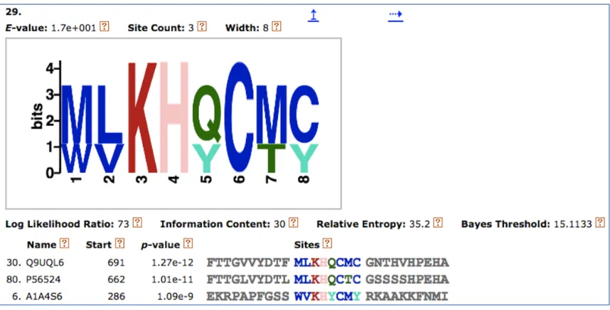
Once the SLiM sets are obtained, MEME outputs files that contain patterns of the SLiMs, sites found in the protein sequences and their positions, and the probability matrix of the features of each SLiM. Figure 3.3.1 shows SLiM No.29 found in the CM dataset as output by MEME with the sites found in the sequences and the corresponding protein names.

Table 1 shows thePosition-specific probability matrix(PSPM) of this SLiM. The columns

represent the 20 amino acids, while the rows correspond to the scores of the features in this SLiM.

We propose five different scoring method variances in this section. Counting sites with different scoring functions and a new approach for defining sites, which we call Sliding Window Scoring method.

FIGURE 3.3.1: SLiM No.29 found in the CM dataset.

3.3.1 Scoring method variance 1: Counting sites

(41)

TABLE 3.3.1: Position-specific probability matrix of SLiM No.29.

A C D E F G H I K L M N P Q R S T V W Y

0 0 0 0 0 0 0 0 0 0 0˙.6 0 0 0 0 0 0 0 0˙.3 0

0 0 0 0 0 0 0 0 0 0˙.6 0 0 0 0 0 0 0 0˙.3 0 0

0 0 0 0 0 0 0 0 1.0 0 0 0 0 0 0 0 0 0 0 0

0 0 0 0 0 0 1.0 0 0 0 0 0 0 0 0 0 0 0 0 0

0 0 0 0 0 0 0 0 0 0 0 0 0 0˙.6 0 0 0 0 0 0˙.3

0 1.0 0 0 0 0 0 0 0 0 0 0 0 0 0 0 0 0 0 0

0 0 0 0 0 0 0 0 0 0 0˙.6 0 0 0 0 0 0˙.3 0 0 0

0 0˙.6 0 0 0 0 0 0 0 0 0 0 0 0 0 0 0 0 0 0˙.3

sequences. As shown in Figure 3.3.2 , Motif 5 appears three times on the sequence of

proteinA0J LT2as three sites being output by MEME, and hence the score of Motif 5 for

A0J LT2is set to 3. Similarly, Motif 16 appears once in the sequence of the same protein

as a site, so the score of Motif 16 for A0JLT2 is set to 1. We applied this scoring method for every protein from the prediction of PPIs.

3.3.2 Scoring method variance 2: Counting sites with

I

formula

After obtaining good experimented results from the scoring method variance 1 mentioned

above, we consider using scoring functions instead of simply counting the SLiMs. Rueda

et al. [29] used SLiMs as properties for prediction of obligate and non-obligate protein interaction complexes. Their prediction results for two datasets showed an impressive

ac-curacy of more than 99% based on classifiers such ask-NN,LDRandSVM. In that paper,

the authors indicate that given a sequenceX of lengthL, they consider an l-mer ain the

sequence as a potential site, wherel is the length of each SLiM. The scoring function they

(42)

FIGURE 3.3.2: Example of obtaining scores using method variance 1 (Counting SLiMs).

we consider to use this I formula as the scoring function for processing the scores of our

SLiMs.

I(a|X) = − l

X

i=1

P(ai)×log(P(ai)) (3.3.1)

whereX is the profile sequence,P(ai)is the probability (of theith residue ofa) from

that profile. SinceP(ai)≤1,

Pl

i=1P(ai)is very small for large sites, so they take -log for

a more meaningful measure [29].

Since log(1) = 0, for anyP(ai)=1, a small threshold is subtracted fromP(ai)as follows

[29]:

logP(ai) =



  

  

log(0.99) ifP(ai) = 1

log(P(ai)) otherwise

(3.3.2)

(43)

we can score this site using theIformula. In the position-specific probability matrix, each line indicates the scores of corresponding features on each position. Therefore, the score

of site MLKHQCMC can be calculaed as I = −(0.6×log(0.6) + 0.6×log(0.6) + 1×

log(0.99) + 0.6×log(0.6) + 1×log(0.99) + 0.6×log(0.6) + 0.6×log(0.6)). We applied this scoring method variance for every protein from the prediction of PPIs.

FIGURE 3.3.3: Example of obtaining scores using method variance 2 (Counting SLiMs

withI formula).

3.3.3 Scoring method variance 3: Counting sites with

I

ˆ

formula

Equation (3.3.1) implies that that larger the site is, the larger the information content is. Thus, in [29], the authors also divide the total information content by the length of the site,

lin order to erase that effect. Then the information content of a siteaof lengthlis defined

as:

ˆ

I(a|X) =−1

l ×

l

X

i=1

P(ai)×log(P(ai)) (3.3.3)

(44)

applied this scoring method for every protein from both of the prediction of PPIs and pre-diction of CaM-binding proteins.

3.3.4 Scoring method variance 4: Counting sites with

I

ˆ

formula /

counting of sites

We consider the length of the sites in the scoring method variance 3, and after we obtained all the scores using this scoring method, we infer that the counting of the sites may affect.

In order to see the influence of the counting of the sites using the Iˆformula, we divided

theIˆformula by the counting of corresponding SLiM. Since we already obtained the score

matrix of the counting of sites, here we divide the element in the matrix, which obtained by method variance 3, by the element in the other matrix, which obtained by method variance 1, in the same position in their own matrix. We applied this scoring method for every protein from both of the prediction of PPIs and prediction of CaM-binding proteins.

3.3.5 Scoring method 5: Sliding Window Scoring method

After we obtained all of the score matrices using different scoring method variances men-tioned above, we thought about a new way to define a site. Thus, we did not consider the sites in the sequences found by MEME. In contrast, we consider every possible

sub-sequence (l-mer) in a sequence as a potential site for a motif of the training set. Each

se-quence is divided into overlappingl-mers. We designed aSliding Window Scoring(SWS)

method for scoring these sites. Figure 3.3.4 shows an example of SWS based on SLiM

No.29 along with its position-specific probability matrix. Let us considerl-mer ain a

se-quence of lengthL. We divide the sequence into all possible overlappingl-mersof length

W, wherel is the length of each SLiM, and deliver a total of{L−W + 1}l-mers. Then,

Equation (3.3.4) is used to calculate the information contained inl-mer a, given a profile

(45)

P(a|X) =

W

X

i=1

P(ai) (3.3.4)

where X is the profile of the sequence, P(ai) is the probability of the amino acid in

that profile. SinceP(a|X)may be 0 or very small if the SLiM and the site have very low

similarity, we set a threshold to 60% forP(a|X). Thus, we do not consider this site and

remove the P(a|X) score as well. Once the scores for all possible l-mers in profileX

are obtained, we use Equation (3.3.5) to add up all the scores of thel-mersas the score of

SLiMmfor profileX:

P(m|X) =

L−W+1 X

i=1

P(a|X) (3.3.5)

Equation (3.3.5) implies that the more likelyais a site, the larger the information

con-tent is. Thus, in order to erase this effect, we also divide the total information concon-tent by

the number of sites in the sequence, N ₆ L−W + 1, since we removed some site with

scores lower than 60%):

ˆ

P(m|X) = 1

N ×

L−W+1 X

i=1

P(a|X) (3.3.6)

Then, we calculate P(m|X)andPˆ(m|X)for all the SLiMs obtained from both CM

and SM datasets for each protein sequence. We applied this scoring method for every protein from both the prediction of PPIs and prediction of CaM-binding proteins.

3.4 Score Processing

(46)

(47)

are single proteins. Figure 3.4.1 shows an example of score processing for prediction of PPIs and CaM-binding proteins.

FIGURE 3.4.1: Example of score processing for prediction of PPIs and CaM-binding pro-teins.

3.4.1 Score processing for prediction of PPIs

For prediction of PPIs using the SWS method, considering we are given a protein pair (Pi,

Pj), si1 tosin are theP(m| X)scores of each SLiM in sequencePi, whilesj1 tosjn are

theP(m|X)scores of each SLiM on sequence of protein Pj, nis the number of SLiMs,

soPi=si1,si2, ... ,sinandPj=sj1,sj2, ... ,sjn. Also, we use thePˆ(m|X)values of each

SLiM on sequencesPi andPj respectively to generateti1 totin andtj1 totjn, where Pi =

ti1, ti2, ... ,tin andPj =tj1, tj2, ... ,tjn. Thus, pair(Pi, Pj)is transformed into two total

score vectors of lengthnas follows:

Sij = (si1+sj1, ..., sin+sjn)

(48)

where Sab and Tab are theP(m| X) and Pˆ(m| X) scores of SLiMb of the sequence of

protein Pa, Sij is the total score matrix of P(m| X) scores for n SLiMs in each protein

sequence pair, andTij is the total score matrix ofPˆ(m|X)scores for the samenSLiMs in

each protein sequence pair. We call the matricesSscore matrix andT score matrix forSij

andTij respectively. This transformation is applied to each positive pair and each negative

pair in the training set with the SLiMs obtained from both CM and SM approaches. Similarly, for prediction of PPIs using method variance 1 to method variance 4, , we also add up the scores between pairs of proteins as the score for each SLiM, and applied this transformation to each pair with the SLiMs obtained from both CM and SM.

3.4.2 Score processing for CaM-binding proteins

As for prediction of CaM-binding proteins using the SWS method, since they are single

proteins, we determine that si1 to sin are the P(m| X) scores of each SLiM on every

sequence of the protein, whileti1 to tin are the Pˆ(m|X) scores of each SLiM on every

sequence of the protein, wherenis the frequency of SLiMs. Thus, each protein sequence

is transformed into two total score vectors of lengthnas follows:

Sij = (si1, si2, ..., sin)

Tij = (ti1, ti2, ..., tin)

whereSi andTi are theP(m|X)andPˆ(m|X)scores of SLiM fornSLiMs on each

protein sequence. We call the matrices S score matrix and T score matrix for Si and Ti

respectively. This transformation is also applied to each positive pair and each negative pair in the training set with the SLiMs obtained from both the SM and CM approaches.

Similarly, we applied the same score processing for prediction of CaM-binding using method variances 3 and 4.

3.5 Machine Learning Method Using for Classification

We appliedSVM-Polynomial kernel,RF,kNN,DT andMPclassifiers on our dataset using

(49)

(50)

Results

We have applied five different scoring methods for prediction of PPIs and CaM-binding proteins, but the results among all of them are quite similar, thus, in this chapter, we analyze and discuss only one scoring method variance, the SWS method, which obtains the best results. We select the best results among all of the results with 5 different classifiers:

SVM-Polynomial with C = 1 and gamma = 0 (c= 1,g = 0), RF, 1-NN, DT, MP.

4.1 Results

As for the SWS method, we have performed eight sets of experiments for both the

predic-tion of PPIs and CaM-binding proteins: classifying the (1)Sand (2)T score matrices with

SLiMs obtained from SM, classifying the (3)Sand (4)T score matrices using the feature

subset selected by FS with SLiMs obtained from SM, classifying the (5)Sand (6)T score

matrices with SLiMs obtained from CM and classifying the (7)Sand (8)T score matrices

using the feature subset selected by FS with SLiMs obtained from CM.

4.1.1 Classification results of prediction of PPIs

Table 4.1.1 shows the classification results for the score matrices with SLiMs obtained from the CM dataset while Table 4.1.2 shows the classification results for the score matrices with SLiMs obtained from the SM dataset.

By observing Tables 4.1.1 and 4.1.2, it is noticed that for the SLiMs obtained from the CM dataset, the classification accuracies range from 67.0% to 84.1% among all of the

(51)

TABLE 4.1.1: Prediction of PPIs classification results for the score matrices with SLiMs obtained from the CM approach.

Dataset for Classification

Classifier Accuracy

(%)

Recall (%) MCC

S score

SVM-Polynomial

(c= 1, g = 0)

76.1 76.1 0.525

Random Forest 76.1 76.1 0.509

k-NN(k = 1) 75.0 75.0 0.488

matrix Decision Tree 64.8 64.8 0.270

Multilayer Perceptron

79.5 79.5 0.586

T score

SVM-Polynomial

(c= 1, g = 0)

79.5 79.5 0.583

k-NN(k = 1) 81.8 81.8 0.651

78.4 78.4 0.557

S score

SVM-Polynomial

(c= 1, g = 0)

78.4 78.4 0.562

matrix subset k-NN(k = 1) 80.7 80.7 0.611

selected by FS Decision Tree 75.0 75.0 0.499

79.5 79.5 0.591

T score

SVM-Polynomial

(c= 1, g = 0)

84.1 84.1 0.675

(52)

TABLE 4.1.2: Accuracies of prediction of PPIs classification for the score matrices with SLiMs obtained from the SM approach.

Classifier Accuracy

(%)

Recall (%) MCC

S score

SVM-Polynomial

(c= 1, g = 0)

73.9 73.9 0.492

k-NN(k = 1) 72.7 72.7 0.439

81.8 81.8 0.632

T score

SVM-Polynomial

(c= 1, g = 0)

56.8 56.8 0.000

k-NN(k = 1) 77.3 77.3 0.533

70.5 70.5 0.390

S score

SVM-Polynomial

(c= 1, g = 0)

70.5 70.5 0.392

77.3 77.3 0.545

T score

SVM-Polynomial

(c= 1, g = 0)

56.8 56.8 0.000

(53)

the highest classification accuracies, ranging from 76.1% to 84.1%. For the SLiMs

ob-tained from the SM dataset, Multilayer Perceptron on theSscore matrix yields the highest

classification accuracy, 81.8%.

4.1.2 Grid search for SVM-polynomial (prediction of PPIs)

We applied grid search using SVM Polynomial on prediction of PPIs for four kinds of matrices datasets as shown in Tables 4.1.3 and 4.1.4 with SLiMs obtained from SM and CM separately, with different values of parameter C = 1, 10, 100, 1000, gamma = 0.01, 0.1, 0, 1, 10, 100, 1,000. We chose 3-fold cross-validation for evaluation.

Observing to Tables 4.1.3 and 4.1.4, we find that after applying grid search for SVM-Polynomial kernel with different values of C and gamma, the accuracy goes up to 84.1% with SLiMs obtained from the CM dataset and it reaches 86.4% with SLiMs obtained from the SM dataset. This means that the value of the parameters plays an important role in our approach.

4.1.3 Classification results of prediction of CaM-binding proteins

Table 4.1.5 shows the classification results for the score matrices with SLiMs obtained from SM while Table 4.1.6 shows the classification results for the score matrices with SLiMs obtained from CM of CaM-binding proteins using the SWS method.

By observing Tables 4.1.5 and 4.1.6, it is noticed that for the SLiMs obtained from SM,

1-NN on the S score matrix yields the highest classification accuracy of 80.6%. For the

SLiMs obtained from CM, the classification accuracies range from 57.6% to 80.1% among

all of the classification experiments. RF on the S score matrix subset after FS yields the

(54)

TABLE 4.1.3: Accuracies (%) of prediction of PPIs using SVM-Polynomial (C = 1, 10, 100, 1000, gamma = 0.01, 0.1, 0, 1, 10, 100, 1000) with SLiMs obtained from SM.

C=1 C=10 C=100 C=1,000

gamma=0 61.4 61.4 61.4 61.4

gamma=0.01 61.4 61.4 61.4 61.4

Sscore gamma=0.1 61.4 61.4 61.4 61.4

gamma=1 61.4 61.4 61.4 61.4

matrix gamma=10 61.4 61.4 61.4 61.4

gamma=100 61.4 61.4 61.4 61.4

gamma=1,000 61.4 61.4 61.4 61.4

gamma=0 56.8 56.8 60.2 71.6

gamma=0.01 56.8 56.8 60.2 71.6

T score gamma=0.1 56.8 60.2 71.6 76.1

gamma=1 59.1 71.6 76.1 71.6

matrix gamma=10 71.6 76.1 72.7 70.5

gamma=100 78.4 78.4 79.5 79.5

gamma=1,000 62.5 63.6 63.6 63.6

gamma=0 61.4 61.4 61.4 61.4

gamma=0.01 63.6 63.6 63.6 63.6

Sscore gamma=0.1 61.4 61.4 61.4 61.4

matrix subset gamma=1 61.4 61.4 61.4 61.4

selected by FS gamma=10 61.4 61.4 61.4 61.4

gamma=100 61.4 61.4 61.4 61.4

gamma=1,000 61.4 61.4 61.4 61.4

gamma=0 56.8 56.8 58.0 69.3

gamma=0.01 56.8 56.8 56.8 56.8

T score gamma=0.1 56.8 56.8 56.8 69.3

gamma=100 72.7 84.1 79.5 78.4

(55)

TABLE 4.1.4: Accuracies (%) of prediction of PPIs using SVM-Polynomial (C = 1, 10, 100, 1000, gamma = 0.01, 0.1, 0, 1, 10, 100, 1000) with SLiMs obtained from CM.

C=1 C=10 C=100 C=1,000

gamma=0 76.1 76.1 76.1 76.1

gamma=0.01 76.1 76.1 76.1 76.1

Sscore gamma=0.1 76.1 76.1 76.1 76.1

gamma=1 76.1 76.1 76.1 76.1

matrix gamma=10 76.1 76.1 76.1 76.1

gamma=100 76.1 76.1 76.1 76.1

gamma=1,000 76.1 76.1 76.1 76.1

gamma=0 79.5 78.4 77.3 77.3

gamma=0.01 68.2 79.5 76.1 77.3

T score gamma=0.1 77.3 77.3 77.3 77.3

gamma=1 77.3 77.3 77.3 77.3

matrix gamma=10 77.3 77.3 77.3 77.3

gamma=100 77.3 77.3 77.3 77.3

gamma=1,000 77.3 77.3 77.3 77.3

gamma=0 78.4 78.4 78.4 78.4

gamma=0.01 78.4 78.4 78.4 78.4

Sscore gamma=0.1 78.4 78.4 78.4 78.4

gamma=100 78.4 78.4 78.4 78.4

gamma=1,000 78.4 78.4 78.4 78.4

gamma=0 84.1 84.1 86.4 84.1

gamma=0.01 56.8 56.8 60.2 85.2

T score gamma=0.1 85.2 84.1 85.2 86.4

gamma=100 75.0 75.0 75.0 75.0

(56)

TABLE 4.1.5: Prediction of CaM-binding proteins classification results for the score ma-trices with SLiMs obtained from SM.

Classifier Accuracy

(%)

Recall (%) MCC

S score

SVM-Polynomial

(c= 1, g = 0)

72.6 72.6 0.453

k-NN(k = 1) 80.6 80.6 0.612

76.0 76.0 0.533

T score

SVM-Polynomial

(c= 1, g = 0)

55.0 55.0 0.105

k-NN(k = 1) 59.7 59.7 0.275

75.7 75.7 0.518

S score

SVM-Polynomial

(c= 1, g = 0)

56.1 56.1 0.122

76.2 76.2 0.545

T score

SVM-Polynomial

(c= 1, g = 0)

64.9 64.9 0.297

(57)

TABLE 4.1.6: Prediction of CaM-binding proteins classification results for the score ma-trices with SLiMs obtained from CM.

Classifier Accuracy

(%)

Recall (%) MCC

S score

SVM-Polynomial

(c= 1, g = 0)

72.6 72.6 0.453

k-NN(k = 1) 78.3 78.3 0.566

76.5 76.5 0.553

T score

SVM-Polynomial

(c= 1, g = 0)

57.6 57.6 0.213

k-NN(k = 1) 58.1 58.1 0.261

71.3 71.3 0.436

S score

SVM-Polynomial

(c= 1, g = 0)

62.0 62.0 0.240

77.0 77.0 0.560

T score

SVM-Polynomial

(c= 1, g = 0)

60.2 60.2 0.210

(58)

4.1.4 Grid search for SVM-polynomial (prediction of CaM-binding

proteins)

Similarly, we applied grid search with different values of parameter C = 1, 10, 100, 1000, gamma = 0.01, 0.1, 0, 1, 10, 100, 1000 on prediction of CaM-binding proteins for the score matrices using SVM-polynomial as shown in Tables 4.1.7 and 4.1.8 with SLiMs obtained from SM and CM separately. We chose 3-fold cross-validation for evaluation.

TABLE 4.1.7: Accuracies (%) of prediction of CaM-binding proteins using

SVM-Polynomial (C = 1, 10, 100, 1000, gamma = 0.01, 0.1, 0, 1, 10, 100, 1000) with SLiMs obtained from SM.

C=1 C=10 C=100 C=1,000

gamma=0 72.6 72.6 72.6 72.6

gamma=0.01 72.6 72.6 72.6 72.6

Sscore gamma=0.1 72.6 72.6 72.6 72.6

gamma=1 72.6 72.6 72.6 72.6

matrix gamma=10 72.6 72.6 72.6 72.6

gamma=100 72.6 72.6 72.6 72.6

gamma=1,000 72.6 72.6 72.6 72.6

gamma=0 55.0 69.8 75.2 73.6

gamma=0.01 55.0 70.3 75.5 73.4

T score gamma=0.1 73.4 70.5 68.0 68.7

gamma=1 68.7 68.7 68.7 68.7

matrix gamma=10 68.7 68.7 68.7 68.7

gamma=100 68.7 68.7 68.7 68.7

gamma=1,000 68.7 68.7 68.7 68.7

gamma=0 45.0 45.0 45.0 45.0

gamma=0.01 42.4 69.3 61.5 61.5

Sscore gamma=0.1 62.8 62.8 62.8 62.8

gamma=100 48.3 48.3 48.3 48.3

gamma=1,000 56.1 56.1 56.1 56.1

gamma=0 53.0 62.5 62.5 62.5

gamma=0.01 53.0 53.0 53.0 53.0

T score gamma=0.1 53.0 62.5 62.5 62.5

gamma=100 64.3 63.6 58.4 64.3

(59)

TABLE 4.1.8: Accuracies (%) of prediction of CaM-binding proteins using SVM-Polynomial (C = 1, 10, 100, 1000, gamma = 0.01, 0.1, 0, 1, 10, 100, 1000) with SLiMs obtained from CM.

C=1 C=10 C=100 C=1,000

gamma=0 72.6 72.6 72.6 72.6

gamma=0.01 72.6 72.6 72.6 72.6

Sscore gamma=0.1 72.6 72.6 72.6 72.6

gamma=1 72.6 72.6 72.6 72.6

matrix gamma=10 72.6 72.6 72.6 72.6

gamma=100 72.6 72.6 72.6 72.6

gamma=1,000

gamma=0 57.6 71.3 72.9 71.3

gamma=0.01 57.6 71.8 72.9 71.3

T score gamma=0.1 71.3 68.5 70.3 70.3

gamma=1 70.3 70.3 70.3 70.3

matrix gamma=10 70.3 70.3 70.3 70.3

gamma=100 70.3 70.3 70.3 70.3

gamma=1,000 70.3 70.3 70.3 70.3

gamma=0 62.0 62.0 62.0 62.0

gamma=0.01 44.7 44.7 44.7 44.7

Sscore gamma=0.1 52.7 52.7 52.7 52.7

gamma=100 55.3 55.3 55.3 55.3

gamma=1,000 33.6 33.6 33.6 33.6

gamma=0 60.2 63.3 64.6 65.6

gamma=0.01 58.1 58.1 58.1 60.2

T score gamma=0.1 60.2 63.3 64.6 65.6

gamma=100 71.8 69.8 67.4 69.8

(60)

Observing Tables 4.1.7 and 4.1.8, we find that after applying grid search for SVM-Polynomial kernel with different values of C and gamma, the accuracy goes up to 72.9% with SLiMs obtained from CM and it reaches 75.5% with SLiMs obtained from SM. Com-pared with the results by SVM-Polynomial with C = 1, gamma = 0, the grid search does not improve the classification results.

4.2 Comparison

4.2.1 Comparison between results of prediction of PPIs

Following the classification results shown in Tables 4.1.1 and 4.1.2, we plot all the accura-cies among the classification results for the four matrices with SLiMs obtained from CM

as shown in Figure 4.2.1. From Figure 4.2.1, we observe that the T score matrix subset

selected by FS obtained the highest accuracies on SVM-Polynomial with C = 1 and gamma

= 0, Random Forest and Decision Tree classifiers. The original T score matrix achieves

the highest accuracy on 1-NN. Most of the accuracies obtained from the T score matrix

are higher than the accuracies obtained from theSscore matrix among different classifiers.

The classifiers perform better after FS on both of theS andT score matrices.

We also compare all the accuracies among the classification results for the four matrices

with SLiMs obtained from SM as shown in Figure 4.2.2. TheS score matrix yielded the

highest accuracies on Multilayer Perceptron, and theT score matrix subset selected by FS

also obtained accuracy which is above 80%.

4.2.2 Comparison between results of prediction of CaM-binding

pro-teins results

Similarly, following the classification results shown in Tables 4.1.5 and 4.1.6, we plot all the accuracies among the classification results for the four matrices with SLiMs obtained

from CM as shown in Figure 4.2.3. From Figure 4.2.3, we observe that theT score

ma-trix subset selected by FS yielded the highest accuracies on Random Forest. Most of the

(61)

FIGURE 4.2.1: Accuracies for prediction of PPIs for matrices with SLiMs obtained from CM.

(62)

score matrices among different classifiers. The classifiers perform better after FS on most

of both of theSandT score matrix.

We also compare all the accuracies among the classification results for the four matrices

with SLiMs obtained from SM as shown in Figure 4.2.4. TheS score matrix obtained the

highest accuracies on 1-NN, while all of the accuracies obtained fromSscore matrices are

higher than the accuracies obtained fromT score matrices among different classifiers.

FIGURE 4.2.3: Accuracies for prediction of CaM-binding for matrices with SLiMs ob-tained from CM.

Table 4.2.5 shows the comparison of prediction of CaM-binding proteins between

re-sults of SM and CM, using the 1-NN classifier. BothS andT score matrices yield higher

accuracies with SM than the matrices with CM using 1-NN classifier, while after FS, both

SandT score matrices yield higher accuracies with CM.

4.2.3 Classification VS Classification + FS

(63)

FIGURE 4.2.4: Accuracies for prediction of CaM-binding for matrices with SLiMs ob-tained from SM.