High speed computing of ice thickness equation for ice sheet model

(1)

78: 8-2 (2016) 143–149 | www.jurnalteknologi.utm.my | eISSN 2180–3722 |

Jurnal

Teknologi

Full Paper

HIGH

SPEED

COMPUTING

OF

ICE

THICKNESS

EQUATION FOR ICE SHEET MODEL

Masyitah Mohd Saidi

a

_{and Norma Alias}

b*

a

_{Department of Mathematical Science, Faculty of Science,}

Universiti Teknologi Malaysia, 81310 UTM Johor Bahru, Johor,

Malaysia

b

_{Center for Sustainable Nanomaterials (CSNano), Ibnu Sina}

Institute for Scientific and Industrial Research, Universiti Teknologi

Malaysia, 81310 UTM Johor Bahru, Johor, Malaysia

Article history Received 14 December 2015 Received in revised form

16 March 2016 Accepted 15 March 2016

*Corresponding author

[email protected]

Graphical abstract

Abstract

Two-dimensional (2-D) ice flow thermodynamics coupled model acts as a vital role for visualizing the ice sheet behaviours of the Antarctica region and the climate system. One of the parameters used in this model is ice thickness. Explicit method of finite difference method (FDM) is used to discretize the ice thickness equation. After that, the equation will be performed on Compute Unified Device Architecture (CUDA) programming by using Graphics Processing Unit (GPU) platform. Nowadays, the demand of GPU for solving the computational problem has been increasing due to the low price and high performance computation properties. This paper investigates the performance of GPU hardware supported by the CUDA parallel programming and capable to compute a large sparse complex system of the ice thickness equation of 2D ice flow thermodynamics model using multiple cores simultaneously and efficiently. The parallel performance evaluation (PPE) is evaluated in terms of execution time, speedup, efficiency, effectiveness and temporal performance.

Keywords: Ice thickness, 2-D ice flow, Finite Difference Method, Explicit Method, CUDA

Abstrak

Gandingan model aliran ais termodinamik dua-dimensi (2-D) mempunyai peranan penting dalam menggambarkan tingkah laku lapisan ais di kawasan Antartica dan sistem iklim. Salah satu parameter yang digunakan di dalam model ini adalah ketebalan ais. Kaedah yang jelas dalam kaedah perbezaan terhingga (FDM) telah digunakan dalam pendiskretan persamaan ketebalan ais. Selepas itu, persamaan itu akan dilaksanakan dalam pengaturcaraan Compute Unified Device Architecture (CUDA) dengan menggunakan Graphics Processing Unit (GPU). Kebelakangan ini, permintaan dalam GPU untuk menyelesaikan masalah pengiraan telah meningkat disebabkan oleh harga yang rendah dan ciri-ciri prestasi pengiraan yang tinggi. Artikel ini bertujuan untuk menyiasat prestasi perkakasan GPU yang disokong oleh pengaturcaraan selari CUDA dan mampu untuk mengira persamaan ketebalan ais dengan menggunakan model aliran ais termodinamik 2D dalam sistem yang besar, jarang dan kompleks. Penilaian prsetasi selari (PPE) dinilai dari segi masa pelaksanaan, kecepatan, kecekapan, keberkesanan dan prestasi sementara.

Kata Kunci: Ketebalan ais, 2-D pengaliran ais, Kaedah Perbezaan Terhingga, Kaedah Jelas, CUDA

thermodynamics model

Ice thickness Equation

Disretization using Explicit FDM

(2)

1.0 INTRODUCTION

Ice sheets are regarded as an important interactive element in the global climate system that can contribute to the increasing of sea level. The water stored and released from ice sheets to the ocean made the sea level is varied in part. The two dominant ice sheets on the Earth are Greenland ice sheet and Antarctica ice sheet. If both of the ice sheets completely melt, the global sea level will be rise about 70 m [1]. While the Antarctica ice sheet alone stored an enormous of water which equivalent to 61 m [2]. Intergovernmental Panel on Climate Change (IPCC) stated that the Antarctica ice sheet contributes to the rate of the increasing sea level about 0.41 mm per year [3].

The modeling of ice sheets is studied to predict the reaction of the ice sheets and simulate the dynamic behaviours of ice sheets numerically. The global sea level can be predicted by the change of the ice sheets behaviours. The evolution and changed of the ice sheets will act as an indicator of the climate. In this paper, 2-D ice flow thermodynamics coupled model is used to observe Antarctica ice sheet evolution. This model is simplified from three dimensional (3-D) Glimmer model and become the 2-D ice flow with the coupled conditions of temperature. The evolution and interaction of thermodynamics governed in this model are in terms of ice thickness, ice velocity and ice temperature. But, this paper focuses on one dimensional (1D) ice thickness equation of the model because it is the main variable in the calculation for the depth-averaged of velocity. Ice thickness also can produce the bedrock elevations by subtracting it from surface elevations.

The aim of this paper is to discretize the ice thickness equation of the model using the explicit finite difference method and performed the numerical calculation by using CUDA on GPU platform for parallel computing. In this era, the utilization of GPU is not only for powerful rendering the graphics, but also can be used for general purpose of non-graphical computing. GPU is outstanding in applying for both graphics and computation purpose. CUDA is the parallel programming with the use of GPU. CUDA has been introduced in 2006 as the first general computing that harnessing general purpose computing on graphics processing unit (GPGPU). This programming has been used by many researchers to solve their problem with the large scale and complex computational in a more efficient way. CUDA is flexible to utilize the resources of GPU due to a unified programming model. The high data-parallelism of CUDA enables to speedup the computation [4]. Thus, this study will be implemented and run the ice thickness equation on two computer models which are C programming on the Central Processing Unit (CPU) and CUDA embedded with C language on GPU. GPU computation platform is chosen to reduce the

execution time of the numerical computations. Then, the parallel performance evaluation (PPE) is measured based on speedup, efficiency, effectiveness and temporal performance. The formula of this PPE refers to [5, 6, 7, 8]. But, CUDA with the shared memory architectures depends on the number of threads per block differ from the distributed memory architectures.

This paper is organized as follows: first, in section 2 discussed about the literature review of the paper. Then, the methodology consists of ice thickness equation with specific parameters, the parallel algorithm for the equation and a brief about CUDA presented in section 3. While in section 4 showed and discussed the results that obtained from the study and lastly in section 5 is concluded the paper.

2.0 LITERATURE REVIEW

(3)

High performance computing on GPU has gained an interest of many researchers from many fields due to the flexible programming for the high floating point performance. In 1999, GeForce 256 was introduced the first GPU for 3-D graphics processors with the single chip. Then, GPU has been evolved from the graphics processor to the programmable processor for parallel which can execute many parallel threads from the multiple cores. GPU becomes more efficient cost. NVIDIA has invented CUDA programming to be implemented on GPU platform [20]. The implementation of the algorithm was using standard C language with CUDA specific extensions. The computations on GPU can be managed by CUDA due to the computing of data-parallel. Today’s, there are many numerical computations that has been computed by using CUDA that utilized GPU to minimize the computational time. In the fluid flow, a compact finite difference method with a higher order is used to obtain the solution by implementing on CUDA [21]. In the study, they compared the results obtained from the CPU in terms of computational time. When the mesh size is bigger, the computational time for GPU is lower than the CPU and it increasing the speedup. They concluded that the fluid flow problem that is solved by using a compact finite difference method can obtain a good speedup when running on GPU. The explicit preconditioned conjugate gradient method is parallelized by using a new proposed parallel technique and performed using CUDA [22]. They discussed the CUDA implementation on the propose technique and stated that the performance of the method can be improved by running on GPU platform with the interface of CUDA programming. The new parallel technique is used to investigate the increasing in the performance of the method. Besides that, CUDA programming is applied in the glaciers and ice sheets modeling [8]. They utilized GPU for the modeling of high order ice dynamics. The model was discretized using finite difference method and the linear system of equations has been solved using Gauss-Seidel method which implemented on CUDA. They showed that GPU has an excellent speedup compared to the CPU.

3.0 METHODOLOGY

In this section, the discretization of the ice thickness equation of the 2-D ice flow thermodynamics coupled model is demonstrated. We also presented an overview of the CUDA programming of GPU.

3.1 Ice Thickness Equation

The mathematical modeling for the ice thickness equation of 2D ice flow thermodynamics coupled model and the physical constant are described as below [23, 24].

      _       

 _u_H

x H D x M t H b (1)

where H is the ice thickness, D is diffusivity, u_b is the bottom of horizontal velocity and M is surface accumulation. It can be assumed that there is zero horizontal velocity, u_b 0, so the equation (1) will be written as .               x H D x M t H (2)

Then, the initial and boundary condition for H and D of equation (2) are carried by

 

8

3 3 4 3 4 0          B l x x

H ,

 

0

0 2

1

 Bl Hlt t

H( ,) , ,

 

8

5 3 4 3 4 3 2 7 20 0           

 B x l x

x

D , Γ

 

0,t D(l,t)0

D ₍₃₎

where , Γ

 

and .

Γ ρg A l km

M

B 2 5 8 2 3 ₀ 750

1 8 3         

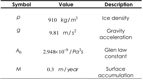
Table 1 The list of the constants used in the model

Symbol Value Description

ρ ₉₁₀ _kg_/_m3 Ice density

g ₉_.₈₁ _m_/_s2 Gravity

acceleration

0

A 9 _Pa3_s

10 948

2.   / Glen law

constant

M 0.3 m/year Surface

accumulation

(4)

        _     _ _  x H H D M t H

H _j _ij _ij

i x j i j i Δ Δ / /2 1 2 1 1                  _ _  x H x H D M t H

H _ij _ij

x j i j i j

i 1 1/2 1/2

Δ                         _          _         x H H D x H H D x M t H H j i j i j i j i j i j i j i j i Δ Δ Δ Δ / / 1 2 1 1 2 1 1 1

 









_                 j i j i j i j i j i j i j i j i H H D H H D x t H t M H 1 2 1 1 2 1 2 1 / / Δ Δ Δ (4) (5) (6) (7)

which is



j



i j i j

i D D

D_₁ ₂  _₁

2 1

/ and

 

. Δ Γ 5 2 1 1 2 5 j i j i j i j

i _x H

H H

D _   

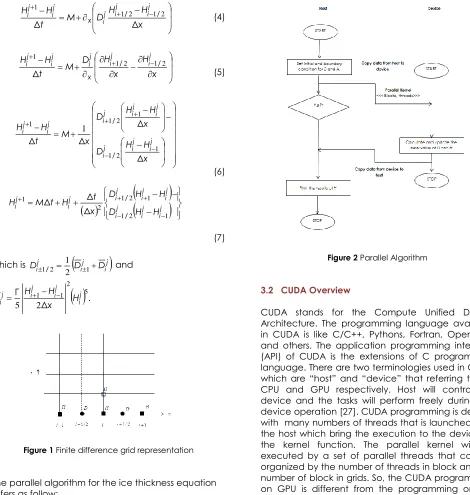
Figure 1 Finite difference grid representation

The parallel algorithm for the ice thickness equation refers as follow:

Figure 2 Parallel Algorithm

3.2 CUDA Overview

CUDA stands for the Compute Unified Device Architecture. The programming language available in CUDA is like C/C++, Pythons, Fortran, OpenACC and others. The application programming interface (API) of CUDA is the extensions of C programming language. There are two terminologies used in CUDA which are “host” and “device” that referring to the CPU and GPU respectively. Host will control the device and the tasks will perform freely during the device operation [27]. CUDA programming is dealing with many numbers of threads that is launched from the host which bring the execution to the device by the kernel function. The parallel kernel will be executed by a set of parallel threads that can be organized by the number of threads in block and the number of block in grids. So, the CUDA programming on GPU is different from the programming on the CPU.

(5)

4.0 RESULTS AND DISCUSSION

Figure 3 Visualization of the distribution of the ice thickness equation

Table 2 Numerical analysis for ice thickness equation

Numerical Analysis Ice thickness Equation Execution time (s) 3.819

Maximum Error 0.171

Root mean square error (RMSE)

0.0428

Number of grid Nx=15, Pt=2500

The ice thickness equation is running on CPU using C programming for sequential algorithm and GPU using CUDA programming for parallel algorithm. Figure 3 shows the results of ice thickness equation computed by numerical and analytical solution of the ice thickness equation in the steady-state [20]. Then, the numerical analysis based on the execution time, maximum error and RMSE are shown in table 2. The graphical graph of numerical solution is approximated to the analytical solution in figure 3 and with the small value of RMSE in table 2 indicate that the numerical method can be used to simulate the ice thickness equation. The execution time of two different computer models and the speedup has been examined based on table 3.

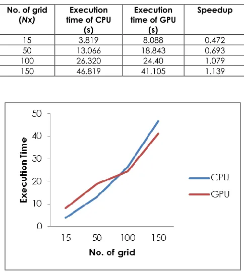
Table 3 Results of Execution time of CPU and GPU and speedup for ice thickness Equation with different number of grid (Nx)

No. of grid

(Nx) time of CPU Execution (s)

Execution time of GPU

(s)

Speedup

15 3.819 8.088 0.472

50 13.066 18.843 0.693 100 26.320 24.40 1.079 150 46.819 41.105 1.139

Figure 4 Execution time of ice thickness equation on CPU and GPU

Figure 5 The value of speedup based on the number of grid

Table 3 and figure 4 shows the execution time of CPU and GPU for ice thickness equation. It is clearly seen that GPU time is much faster than CPU time when the number of grid is increased. Then, figure 5 shows the speedup obtained by comparing GPU time with CPU time and the result shows that the speedup is increasing with the increasing of the number of grid. It can be stated that the

//Define CUDA kernel on Device

__global__void thickness (argument list); {

int i = blockIdx.x*blockDimx +

threadIdx.x; }

//CUDA kernel launch on GPU

(6)

implementation of ice thickness equation on CUDA programming can achieve a good speedup. This is due to the sequential programming on CPU needs to wait the process one by one but for parallel programming on GPU is dividing the computation data by using the number of threads and run simultaneously. Even though the data in this paper is consider small, our goal is to see that the ice thickness equation can be implementing on CUDA programming and reduce the computational time when the data is increased.

Table 4 Execution time of GPU with the different number of threads per block for the number of grid of 150

Threads per block Execution time of GPU (s)

1 227.389

4 85.618

8 60.311

16 44.198

32 47.04

64 49.559

128 49.593

The PPE of ice thickness equation is shown in table 4 and figure 6. In table 4, the results show the execution time of GPU for 150 grids with the different number of threads. Then, in figure 6, we can see the decreasing of the value of effectiveness as the number of the threads per block increasing. It is because of the asynchronous CPU-GPU memory transfers with a bandwidth problem. The temporal performance in CUDA that indicate then, it can be seen that 16 is an optimal number of thread for ice thickness equation from the graph of temporal performance and the execution time of GPU is smaller than CPU.

(a)

(b)

(c)

(d)

Figure 6 Parallel performance evaluation of ice thickness equation based on a) speedup b) efficiency c) effectiveness and d) temporal performance

5.0 CONCLUSION

(7)

outperform the CPU in terms of execution time when the size of the data is increasing. This is due to the CUDA programming suitable for the massively parallel programming and can accommodate to execute many or even up to thousands number of threads simultaneously. Also, the good speedup is achieved in this study that can accelerate the computational time by using CUDA on GPU platform.

Acknowledgement

This research is supported by the Ministry of Higher Education (MOHE), Research Management Centre (RMC) UTM, Ministry of Science, Technology and Innovation Malaysia (MOSTI) and for the financial funded under Research University Grant (4L131). The authors thank the Center for Sustainable Nanomaterials (CS Nano), Ibnu Sina Institute and Universiti Teknologi Malaysia (UTM) for its excellent support for this research.

References

[1] Huybrechts, P., Gregory, J., Janssens, I. and Wild, M. 2004.

Modelling Antarctic and Greenland Volume Changes During The 20th And 21st Centuries Forced By GCM Time

Slice Integrations. Global and Planetary Change. 42:

83-105.

[2] Huybrechts, P., Steinhage, D., Wilhelms, F., Bamber, J. L.

2000. Balance Velocities And Measured Properties Of The Antarctic Ice Sheet From A New Compilation Of Gridded

Datasets For Modeling. Annals of Glaciology. 30: 52–60.

[3] IPCC-AR5, Fifth Assessment Report: Climate Change 2013:

The Physical Science Basis. IPCC, 2013.

[4] Zhang, K., Lu, J., Lafruit, G., Lauwereins, R. and Gool, L. V.

2011. Real-Time And Accurate Stereo: A Scalable

Approach With Bitwise Fast Voting On CUDA. IEEE

Transactions on Circuits and Systems for Video Technology. 2(7): 867-878.

[5] Alias, N., et al., 2011. Performance Evaluation Of

Multidimensional Parabolic Type Problems On Distributed

Computing Systems.2011 IEEE Symposium on Computers

and Communications (ISCC).

[6] Alias, N. and M. R. Islam, 2010. A Review Of The Parallel

Algorithms For Solving Multidimensional PDE Problems.

Journal of Applied Sciences. 10(19): 2187-2197.

[7] Alias, N., et al., 2009. Parallelization of Temperature

Distribution Simulations for Semiconductor and Polymer Composite Material on Distributed Memory Architecture.

Parallel Computing Technologies. Proceedings. 5698:

392-398.

[8] Brædstrup, C. F., Damsgaard, A. and Egholm, D. L. 2014.

Ice - Sheet Modelling Accelerated By Graphics Cards.

Computers & Geosciences. 72: 210–220.

[9] Robin, G. de Q. 1955. Ice Movement And Temperature

Distribution In Glaciers And Ice Sheets. J. GIaciology. 2:

523-532.

[10] Budd, W. F. Jenssen, D. and Radok, U. 1971. Derived

Physical Characteristics Of The Antarctic Ice Sheet, ANARE

Interim Report. Glaciology Publication. 120: 178.

[11] Budd, W. F. and Jenssen, D. 1975. Numerical Modelling Of

Glacier Systems. IAHS Publication. 104: 257-291.

[12] Mahaffy, M. W. 1976. A Three-Dimensional Nurnerical

Rnodel Of Ice Sheets: Tests On The Barnes Ice Cap,

Northwest Territories, J. Geophvs. Res. 81(6): 1059-1066.

[13] Hutter, K., Yakowitz, S. and Szidarovszky, F. 1986. A

Nurnerical Study Of Plane Ice-Sheet Flow. IJ. GIaciol.

32(1111): 139-160.

[14] Hindmarsh, R. C. A., Boulton, G. S. and Hutter, K. 1989.

Modes Of Operation Of Thermo-Mechanically Coupled

Ice Sheets. Ann. Glaciol. 12: 57-69.

[15] Oerlernans, J. 1982a. Response of the Antarctic ice sheet

To A Clirnatic Warrning: A Rnodel Study. J.CIimat. 2: 1-11.

[16] Oerlernans, J. 1982b. A Rnodel Of The Antarctic Ice Sheet.

Nature. 297: 550-553.

[17] Payne A. J. 1999. A Thermomechanical Model Of Ice Flow

in West Antarctica. Climate Dynamics. 15: 115–25.

[18] Bueler, E., Brown, J. and Lingle, C. 2007. Exact Solutions To

The Thermomechanically Coupled Shallow-Ice

Approximation: Effective Tools For Verification. Journal of

Glaciology. 53: 499-516.

[19] Jamieson, S. S. R., Hulton, N. R. J. and Hagdorn, M. 2008.

Modelling Landscape Evolution Under Ice

Sheets. Geomorphology. 97: 91-108.

[20] NVIDIA, 2009a. CUDA Architecture, Introduction &

Overview, Version 1.1.

[21] Tutkun, B. and Edis, F.O. 2012. A GPU Application For

High-Order Compact Finite Difference Scheme. Computers &

Fluids. 55: 29-35.

[22] Gravvanis, G. A, Filelis-Papadopoulos, C. K. and

Giannoutakis, K. M. 2012. Solving Finite Difference Linear Systems On Gpus: Cuda Based Parallel Explicit Preconditioned Biconjugate Conjugate Gradient Type

Methods. Journal Supercomputing. 61: 590-604.

[23] Tang, X., Zhang, Z., Sun, B., Li, Y., Li, N., Wang, B. and

Zhang, X. 2008. Antarctic Ice Sheet GLIMMER Model Test

And Its Simplified Model On 2-Dimensional Ice Flow.

Progress in Natural Science. 18: 173–180.

[24] Alias, N., Kasmin, B. N. K. and Mahmud, N. A. 2014. Some

Numerical Methods for Ice Sheet Behaviour and Its

Visualization. J. Appl. Environ. Biol. Sci. 4(8S): 351-357.

[25] Van Der Veen, C. J. 1999. Fundamentals Of Glacier

Dynamics. Balkeema.

[26] Huybrechts, P. and et. al. 1996. The EISMINT Benchmarks

For Testing Ice–Sheet Models. Annals Glaciology. 23: 1–12.