ABSTRACT
KONG, DEHAN. Penalized Regression Methods with Application to Domain Selection and Outlier Detection. (Under the direction of Howard Bondell and Yichao Wu.)
Variable selection is one of the most important problems in statistical literature, and a popular method is the penalized regression. In this dissertation, we investigate two types of variable selection problems via penalized regression. The first problem is related to the domain selection for the varying coefficient model, which identifies important regions of the varying coefficient that are related to the response. The second problem is related to variable selection problem for the linear model with the existence of outliers, and deal with variable selection and outlier detection simultaneously.
©Copyright 2013 by Dehan Kong
Penalized Regression Methods with Application to Domain Selection and Outlier Detection
by Dehan Kong
A dissertation submitted to the Graduate Faculty of North Carolina State University
in partial fulfillment of the requirements for the Degree of
Doctor of Philosophy
Statistics
Raleigh, North Carolina
2013
APPROVED BY:
Yichao Wu Wenbin Lu
Arnab Maity Howard Bondell
DEDICATION
BIOGRAPHY
ACKNOWLEDGEMENTS
I would express my deepest gratitude to my advisors, Dr. Howard Bondell and Dr. Yichao Wu, for their insightful guidance, generous support and kind encouragement, without which I wouldn’t have achieved what I have now. I would also like to thank Dr.s Wenbin Lu, Arnab Maity and Barbara Sherry for their service on my committee. I am very thankful to Dr. Rui Song, who attends my final oral defense.
I really appreciate the precious learning opportunity and environment provided by the Department of Statistics at North Carolina State University. I would also like to thank all my friends. We shared many great moments in the department, and with their supports and encouragements, I was able to go through many difficult situations.
I am extraordinarily grateful to the Nankai University, especially the Special Class of Math-ematics in honor of Shiing-Shen Chern, where I took various basic mathMath-ematics courses, which helps me a great deal with my research.
TABLE OF CONTENTS
LIST OF TABLES . . . vii
LIST OF FIGURES . . . .viii
Chapter 1 Introduction and Background . . . 1
1.1 An overview of variable selection methods . . . 1
1.2 An overview of the local polynomial regression . . . 2
1.3 An overview of the robust regression . . . 3
Chapter 2 Domain selection for the varying coefficient model via local poly-nomial regression . . . 4
2.1 Introduction . . . 4
2.2 Local polynomial regression for the varying coefficient model . . . 6
2.2.1 Choosing the bandwidth h . . . 7
2.3 Penalized local polynomial regression estimation . . . 8
2.3.1 Algorithms . . . 10
2.3.2 Tuning of the regularization parameter . . . 10
2.4 Asymptotic properties . . . 11
2.5 Simulation example . . . 12
2.5.1 Example 1 . . . 13
2.5.2 Example 2 . . . 14
2.6 Real data application . . . 15
Chapter 3 Fully efficient robust estimation, outlier detection and variable se-lection via penalized regression . . . 19
3.1 Introduction . . . 19
3.2 Methodology . . . 20
3.2.1 Robust Initial Estimator . . . 21
3.2.2 Algorithm . . . 22
3.2.3 Tuning parameter selection . . . 22
3.3 Theoretical results . . . 23
3.3.1 Asymptotic theory when there are no outliers . . . 23
3.3.2 High breakdown point . . . 25
3.3.3 Outlier detection consistency . . . 26
3.4 Simulation Studies . . . 28
3.5 Real data application . . . 29
3.6 Extension to the high dimensional case . . . 31
Chapter 4 Discussions and Future work. . . 33
4.1 Extension of the Domain selection for the varying coefficient model . . . 33
REFERENCES . . . 39
APPENDICES . . . 44
Appendix A Proof in Chapter 2 . . . 45
A.1 Lemmas . . . 45
A.2 Proof of Lemmas . . . 46
A.3 Proof of Theorems and Corollary . . . 48
Appendix B Proof in Chapter 3 . . . 53
B.1 Lemmas and Proofs . . . 53
LIST OF TABLES
Table 2.1 Simulation results for the univariate case using penalized local polynomial regression and original local polynomial regression when sample size varies fromn= 100,200,500. The entries in the table denotes mean square error (MSE) of the estimated function, the correct zero coverage (correctzero) and the estimation error (EE) for the entire model. . . 14 Table 2.2 Simulation results for the multivariate case using penalized local
poly-nomial regression and original local polypoly-nomial regression when sample size varies from n= 100,200,500. The entries in the table denotes mean square error of the estimated functiona1(·) (MSE (function 1)) anda2(·)
(MSE (function 2)), the correct zero coverage (correctzero) fora1(·)
(cor-rectzero(function 1)) and a2(·) (correctzero(function 2)), and the
estima-tion error (EE) for the entire model. . . 15
LIST OF FIGURES
Figure 2.1 Plots of a1(u) (left) anda2(u) (right) for simulation example. . . 13
Figure 2.2 Histogram for √LST AT. . . 16 Figure 2.3 The penalized local polynomial estimates for the coefficient functions.
Chapter 1
Introduction and Background
1.1
An overview of variable selection methods
Variable selection is an important topic in statistical applications. Different classical methods have been introduced such as best subset selection, forward selection, backward elimination and stepwise selection. These methods provide some candidate models through different algorithms and then compare the performance of these models through some criteria, for example the Akaike Information Criterion (AIC) and the Bayesian Information Criterion (BIC). These clas-sical selection methods are intuitive, simple to implement and work well in practice. However, they also suffer from several drawbacks. First, they are not stable, i.e. a small perturbation of the data may result in very different models being selected. Second, it is difficulty to establish the asymptotic properties of the estimator. Third, these methods are computational expen-sive for many modern statistical problems, especially for the high dimensional data where the dimension of the predictor is higher than the sample size.
Recently, the shrinkage method is developed that revolutionizes the variable selection. Sup-pose we have datay= (y1, . . . , yn)⊤,X= (X1⊤, . . . ,X⊤n)⊤ whereXi is ap-dimensional vector. Let L(β;y,X) be the loss function for the data (y,X) with some p-dimensional parameter β= (β1, . . . , βp)⊤, we solve min
β [L(β;y,X) +Pλ(β)], wherePλ is called the penalty function.
The most popular shrinkage method used for variable selection is the least absolute shrinkage and selection operator (Lasso) [50], which adopts an L-1 penalty functionPλ(β) =
∑p
j=1Pλ(βj) = λ∑pj=1|βj|. The Lasso penalty may shrink some of the components ofβto zero, which achieves variable selection. However, Lasso estimator would create bias for nonzero components. To rem-edy this issue, [15] proposed the Smoothly Clipped Absolute Deviation (SCAD) penalty. For each βj, the derivative of the SCAD penalty function is given by
Pλ′(βj) =λ{I(|βj| ≤λ) +(aλ− |βj|)+
and the penalty function itself satisfies Pλ(0) = 0. Unlike the Lasso penalty, SCAD penalty functions have flat tails, which reduce the biases. The estimator possesses three good properties: sparsity, unbiasedness and continuity, which are also called the oracle property. Another variable selection technique enjoying the oracle property is Adaptive Lasso, proposed by [61]. Unlike the Lasso penalty term λ∑pj=1|βj|, they introduced the weighted penalized term λ∑pj=1wj|βj| and recommended usingwj = 1/|βˆj|γ with some γ ≥0, where ˆβj is the least square estimate. There are some other penalized regression methods such as the nonnegative garrote [3], the bridge regression [21], the elastic net [62] and the minimax concave penalty (MCP) [58], among others.
For all these penalized regression methods, they involve a tuning parameterλ, which controls the size of the model. There are several criteria such as cross validation (CV), generalized cross validation (GCV), AIC, BIC and so on. For the SCAD penalty, [51] pointed out that CV, GCV or AIC may result in an overfitting. They advocated the BIC tuning parameter selector, which could identify the true sparse model consistently. Consequently, BIC is preferred for the SCAD penalty, which is also used in Chapter 2 of the thesis when we apply the SCAD penalty.
1.2
An overview of the local polynomial regression
Local polynomial regression is a useful technique for nonparametric smoothing. Simply speak-ing, local polynomial regression fits a weighted polynomial regression in some neighborhood of the pointx0 to obtain the function estimate at x0. We will have an brief overview of the local
polynomial regression here, and for a complete review, see the well written book [13]. Suppose {(xi, yi),1≤i≤n}are pairs of data following
yi = f(xi) +σ(xi)ϵi,
where ϵi are assumed to be independent and identically distributed (iid) standard normal. To estimate f(x) at a fixed point x0, we may use Taylor’s expansion:
f(x)≈f(x0) +f′(x0)(x−x0) +. . .+
f(p)(x0)
p! (x−x0) p
We can estimate f(x0), f′(x0), . . . f(p)(x0) by minimizing the following objective function
min β0,β1,...,βp
n
∑
i=1 {yi−
p
∑
j=0
βj(xi−x0)j}2Kh(xi−x0), (1.1)
K(·/h)/h, where K(·) is a kernel function. The kernel function is defined as a nonnegative symmetric density function satisfying∫ K(t)dt= 1. There are numerous choices for the kernel function, examples include Gaussian kernel, Epanechnikov kernel and others.
Denote the solution of (1.1) as ˆβ = ( ˆβ1, . . . ,βˆp)⊤, we have ˆf(r)(x0) = r! ˆβr for 0 ≤ r ≤p. DenoteXas an×(p+ 1) matrix withijth element (xi−x0)j−1,W be an×ndiagonal matrix
withiith elementKh(xi−x0) and y= (y1, . . . , yn)⊤, we have ˆβ= (X⊤WX)−1X⊤Wy. As the diagonal matrixWis related toh, the estimates of the function depend on the choice of the bandwidth. Since the bandwidth controls the size of the neighborhood, it is essential in lo-cal polynomial fitting. There are various literatures on how to select the appropriate bandwidth. The basic idea is to minimize the Mean Integrated Squared Error (MISE), which is calculated by integrating the conditional Mean Square Error (MSE) over the domain of {xi,1 ≤i≤n}. Various approaches can be used including cross validation, rule of thumb and some multi-stage methods. We will discuss some of these methods in Chapter 2, and for a complete review, we direct the readers to [13].
1.3
An overview of the robust regression
Consider the linear regression model
yi = Xiβ+ϵi,
whereXi is ap dimensional predictor, βis ap×1 parameter, andϵi are the random error iid with mean zero. The Ordinary Least Squares (OLS) estimates are fully efficient when the error follows a normal distribution. However, when the errors deviate from the normal distribution or some outliers exist, OLS estimates may perform very badly. To remedy this issue, various robust regression methods can be used. Basically, these methods work better than OLS estimates as they are not influenced much by the outliers.
Chapter 2
Domain selection for the varying
coefficient model via local
polynomial regression
2.1
Introduction
In this paper, we consider the varying coefficient model [6, 27], which assumes that the covariate effect may vary depending on the value of an underlying variable, such as time. The varying coefficient model is used in a variety of applications such as longitudinal data analysis. The varying coefficient model is given by:
Y = x⊤a(U) +ϵ, (2.1)
with E(ϵ) = 0, and Var(ϵ) = σ2(U). The predictor x = (x1, . . . , xp)⊤, represents p features,
and correspondingly, a(U) = (a1(U), . . . , ap(U))⊤ denotes the effect of each feature over the domain of the variableU.
For model (2.1), there are various proposals for estimation, for example local polynomial smoothing [13, 55, 28, 35, 20], polynomial splines [30, 31, 29], and smoothing splines [27, 28, 5]. In this paper, we will not only consider estimation for the varying coefficient model, but also we wish to identify which regions in the domain ofU for which predictors have an effect and those regions where it may not. This is similar, although different than variable selection, as selection methods attempt to decide whether a variable is active or not while our interest focuses on identifying regions.
Absolute Deviation (SCAD) [15], adaptive lasso [61] and excessively others. Although the lasso penalty gives sparse solutions, the estimates can be biased for large coefficients due to the lin-earity of the L1 penalty. To remedy this bias issue, [15] proposed the SCAD penalty and showed that the estimators enjoy the oracle property in the sense that not only it can select the correct submodel consistently, but also the asymptotic covariance of the estimator is the same as the asymptotic covariance matrix of the ordinary least squares (OLS) estimate as if the true subset model is known as a priori. To achieve the goal of grouped variable selection, [57] developed the group lasso penalty which penalized coefficients as a group in situations such as a factor in ANOVA. As with the lasso, the group lasso estimators do not enjoy the oracle property. As a remedy, [53] proposed the group SCAD penalty, which again selects the variables in a group manner.
For the varying coefficient model, existing works focus on identifying the nonzero coefficient functions, which achieves component selection for the varying coefficient functions. However, each coefficient function is either zero everywhere or else nonzero everywhere. For example, [54] considered the varying coefficient model under the framework of a B-spline basis and used the group SCAD to select the significant coefficient functions. [52] combined local constant regression and the group SCAD penalization together to select the components, while [37] directly applied the component selection and smoothing operator [38].
In this paper, we consider a different problem, detecting the nonzero regions for each com-ponent of the varying coefficient functions. Specifically, we would select the nonzero domain of each aj(U), which corresponds to the regions where the jth component of x has an effect on Y. To this end, we incorporate local polynomial smoothing together with penalized regression. More specifically, we combine local linear smoothing and the group SCAD shrinkage method into one framework, which selects the nonzero regions for the coefficient functions and esti-mates them simultaneously. In this method, we deal with two tuning parameters, namely the bandwidth used in local polynomial smoothing and the shrinkage parameter used in the regu-larization method. We propose methods to select these two tuning parameters. Our theoretical results show that the resulting estimators have the same asymptotic bias and variance as the original local polynomial regression estimators.
2.2
Local polynomial regression for the varying coefficient model
Suppose we have independent and identically distributed (iid) samples {(Ui,x⊤i , Yi)⊤, i = 1, . . . , n} from the population (U,x⊤, Y)⊤ satisfying model (2.1). As a(u) is a vector of un-specified functions, a smoothing method must be incorporated for estimation. In this article, we adopt the local linear approximation for this varying coefficient model [19]. For U in a small neighborhood ofu, we can approximate the function aj(U), 1≤j ≤p, locally by linear regression
aj(U)≈aj(u) +a′j(u)(U−u).
For a fixed point u, denoteaj andbj asaj(u) anda′j(u) respectively, and denote the estimates of aj(u) and a′j(u) as ˆaj and ˆbj, which give the function estimate and the derivative estimate respectively for the functionaj(·) at the pointu. For (ˆaj,ˆbj) (1≤j≤p), they can be estimated via local polynomial regression by solving the following optimization problem:
min
a,b
n
∑
i=1
{Yi−x⊤i a−x⊤i b(Ui−u)}2(Kh(Ui−u)/Kh(0)), (2.2)
wherea= (a1, . . . , ap)⊤andb= (b1, . . . , bp)⊤,Kh(t) =K(t/h)/h, andK(t) is a kernel function. The parameterh >0 is the bandwidth controlling the size of the local neighborhood. The model complexity is controlled by the bandwidthh, consequently choosing the bandwidth is essential in local polynomial regression. We will discuss how to select the bandwidthh in section 2.2.1.
The kernel functionK is a nonnegative symmetric density function satisfying∫K(t)dt= 1. There are numerous choices for the kernel function, examples include Gaussian kernel (K(t) =
1
√
2πexp(−t
2/2)), Epanechnikov kernel (K(t) = 0.75(1−t2)
+) and others. Typically, the
es-timates are not sensitive to the choice of the kernel function. In this paper, we will use the Epanechnikov kernel, which leads to computational efficiency due to its bounded support.
Notice here our loss function is slightly different from the loss function of the traditional local polynomial regression for varying coefficient model [19]. We have rescaled the original loss function by a termKh(0). For a fixedh, this change does not affect the estimates. However, this scaling is needed later to correctly balance the loss function and penalty term sinceKh(Ui−u) = K(Ui−u
h )/h, we include the termKh(0) to eliminate the effect ofhso that Kh(Ui−u)/Kh(0) = O(1).
Denote a0 = (a10, . . . , ap0)⊤ and b0 = (b10, . . . , bp0)⊤ as the true value of the function
values and true derivative values and ˆa = (ˆa10, . . . ,ˆap0)⊤ and ˆb = (ˆb10, . . . ,ˆbp0)⊤ as the local
diag(U1−u, . . . , Un−u), where diag(u1, . . . , un) denotes the matrix with (u1, . . . , un) on the diagonal and zeros elsewhere. Let x(j) be the jth column of X and xij be the ijth element of
X. Denote Γuj = (x(j),Uux(j)) for 1 ≤j ≤ p and Γu = (Γu1, . . . ,Γup) to be a n×p matrix. Define Y = (Y1, . . . , Yn)⊤ and Wu = diag(Kh(U1−u)/Kh(0), . . . , Kh(Un−u)/Kh(0)). Using this notations, we can write (2.2) as
min
γ (Y−Γuγ)
⊤W
u(Y−Γuγ). (2.3)
This notation then has a formulation of a weighted least square problem.
2.2.1 Choosing the bandwidth h
The standard approach to choose the bandwidth is based on the trade-off between the bias and variance. The simplest way is the rule of thumb, see [13] for details. It is fast in computation, however, it highly depends on the asymptotic expansion of the bias and variance, and may not work well in small samples. Moreover, the optimal bandwidth is based on several unknown quantities, for which good estimates may be difficult to obtain. To overcome these deficiencies, we adopt the mean square error (MSE) tuning method. For a detailed review, see [19] and [59]. This method uses information provided with finite samples and hence carries more information about the finite sample, which selects the bandwidth more accurately than other methods such as residual squares criterion (RSC) [12] and cross validation (CV).
The M SE(h) for a fixed smoothing bandwidth h is defined as
M SE(h) = E{x⊤ˆa(U)−x⊤a(U)}2.
By direct calculation, we have
M SE(h) = E[B⊤(U)Ω(U)B(U) + tr{Ω(U)V(U)}], (2.4)
whereB(U) = Bias(ˆa(U)), Ω(U) =E(xx⊤|U) andV(U) = Cov(ˆa(U)). To estimateM SE(h), we need to estimate B(U), Ω(U) and V(U). Then we have
d
M SE(h) =n−1 n
∑
i=1
[ ˆB⊤(Ui) ˆΩ(Ui) ˆB(Ui) + tr{Ω(Uˆ i) ˆV(Ui)}].
kernel smoother
ˆ Ω(u) =
∑n
i∑=1xix⊤i Kh(Ui−u) n
i=1Kh(Ui−u)
Introduce the p×2p matrix M, where the (j,2j −1) (1 ≤ j ≤ n) elements of M are 1, and the remaining elements are 0. [20] summarized the forms of the bias and variance. For the estimated bias, we have
ˆ
B(u) =bias(ˆˆ a(u)) =M(Γ⊤uWuΓu)−1Γ⊤uWuτˆ,
where theith element of ˆτ is
2−1x⊤i {ˆa(2)(u)(Ui−u)2+ 3−1ˆa(3)(u)(Ui−u)3}.
The preceding representation involves two unknown quantities ˆa(2)(u) and ˆa(3)(u), which can
be estimated by local cubic fitting with an appropriate pilot bandwidthh∗. The estimated variance is given by
ˆ
V(u) = cov(ˆˆ a(u)) =M(Γ⊤uWuΓu)−1(Γ⊤uWu2Γu)(Γ⊤uWuΓu)−1M⊤ˆσ2(u).
The estimator ˆσ2(u) can be obtained as a byproduct when we use local cubic fitting with a pilot bandwidth h∗. Denote Γ∗uj = (x(j),Uux(j),U2ux(j),U3ux(j)) and Γ∗u = (Γ∗u1, . . . ,Γ∗up). We have
ˆ
σ2(u) = Y ⊤{W∗
u −Wu∗Γ∗u(Γ∗⊤u Wu∗Γ∗u)−1Γ∗⊤u Wu∗}Y tr{Wu∗−(Γ∗⊤u Wu∗Γ∗u)−1(Γ∗⊤
u Wu∗2Γ∗u)} whereWu∗ isWu withh replaced by h∗.
For the pilot bandwidthh∗, which is used for a pilot local cubic fitting, [12] introduced the RSC to select it. However, they only studied the univariate case, which applies to the varying coefficient model with one component. As we are considering the varying coefficient model with several components, their method is not applicable. Instead, we use five-fold cross validation to do the pilot fitting.
2.3
Penalized local polynomial regression estimation
over certain regions, the derivative should also behave so. Consequently, we treat each (aj, bj) (1≤j ≤p) as a separate group and do penalization together. To achieve the variable selection as well as estimation accuracy, a group SCAD penalty [53] is then added to (2.2) to get sparse solutions fora and b.
Recall that we need to solve the minimization problem (2.3), which can be rewritten as a least square problem with new data (Wu1/2Y, Wu1/2Γu):
min
γ (W
1/2
u Y−Wu1/2Γuγ)⊤(Wu1/2Y−Wu1/2Γuγ).
For a traditional linear model, the covariates would be scaled first before adding the penalty. A similar procedure would be applied by making each column of the covariate Wu1/2Γu have the same variance. Denote sj as the standard deviation for the pseudo covariatesxij(Kh(Ui− u)/Kh(0))1/2 (1≤i≤n) andrj as the standard deviation for the pseudo covariates xij(Ui− u)(Kh(Ui−u)/Kh(0))1/2 (1≤i≤n). In other words, (s1, r1, s2, r2, . . . , sp, rp)⊤are the standard deviations for each column of the pseudo covariate Wu1/2Γu. We would ideally standardize the covariates and do the penalization. In fact, this is equivalent to keeping the covariates the same and change the penalty by reparameterization.
In typical situations, this rescaling is needed only for finite sample behavior. However, in this case, the convergence rates for function estimation, ˆa, and derivative estimation, ˆb are of different orders of magnitude. Hence this rescaling is also necessary asymptotically. We have shown in Lemma 1 in the Appendix that sj =OP(1) andrj =OP(h), which properly adjusts the effect of the different rates of convergence of the function and derivative estimates.
For the local polynomial regression, it is no longer appropriate to use nas the sample size, as not all observations contribute equally to a given location. In fact, some will contribute nothing if the kernel has bounded support. Consequently, we define the effective sample size as m =
∑n
i=1Kh(Ui−u)
Kh(0) . The penalized local polynomial regression estimates (ˆa
⊤
λ,bˆ⊤λ)⊤ can be found by minimizing
min
a,b[
n
∑
i=1
{Yi−x⊤i a−x⊤i b(Ui−u)}2(Kh(Ui−u)/Kh(0)) +m p
∑
j=1
Pλ(
√
s2
ja2j +r2jb2j)], (2.5)
where the SCAD penalty function [15] is a symmetric function at zero which satisfiesPλ(0) = 0 and its first order derivative is defined as
Pλ′(t) =λ{I(t≤λ) +(aλ−t)+
(a−1)λ I(t > λ)} for somea >2 and t >0
coefficients, a set of dense grid is chosen over the whole domain ofU, say (u1, . . . , uN). We can obtain the estimates ofa(u) on these grid points. If the estimate of certain component function is zero for a certain number of consecutive grid points, for instance, say estimate of aj(u) is zero on grid points{ul1, ul1+1, . . . , ul2}. We would say the estimate of the functionaj(u) is zero
over the domain [ul1, ul2].
We will introduce some notations which would be used in the following sections. Denoteβj = (sjaj, rjbj)⊤andβ= (β1⊤, . . . ,β⊤p)⊤. Letβ0 be the true value ofβ. Denote ˆβ= ( ˆβ
⊤
1, . . . ,βˆ
⊤ p)⊤ to be the local polynomial estimates of β0 = (β⊤10, . . . ,β⊤p0)⊤, and ˆβλ = ( ˆβ⊤λ1, . . . ,βˆ⊤λp)⊤ to be the penalized local polynomial estimates when the regularization parameter isλ.
2.3.1 Algorithms
We would discuss how to solve (2.5) in this subsection. For the SCAD penalization problem, [15] proposed the local quadratic approximation(LQA) algorithm to get the minimizer of the penalized loss function. With LQA, the optimization problem can be solved using a modified Newton-Raphson algorithm. The LQA estimator, however, cannot achieve sparse solutions. A threshold would then be used to shrink the small coefficients to zero. To remedy this issue, [63] proposed a new approximation method based on local linear approximation (LLA). The advantange of the LLA algorithm is that it inherits the computational efficiency of LASSO. Denote β(jk) = (sja(jk), rjb(jk))⊤. Given the estimate {βˆ
(k)
j , j = 1, ..., p} at the kth iteration, we minimize
min a,b[
n
∑
i=1
{Yi−x⊤i a−x⊤i b(Ui−u)}2(Kh(Ui−u)/Kh(0)) +m p
∑
j=1
w(jk)||βj||],
to get{βˆ(jk+1), j = 1, ..., p}, wherewj(k) =|Pλ′(||βˆ(jk)||)|. Repeat the iterations until convergence, and the limit would be the minimizer. The initial value of ˆβ(0)j can be chosen as the unpenalized local polynomial estimates. We have found that one step estimates already perform very well, so it is not necessary to iterate further, see [63] for similar discussions. Consequently, the one step estimate is adopted because it can save the computational time.
2.3.2 Tuning of the regularization parameter
When tuning the regularization parameter λ, we adopt the Bayesian information criterion (BIC). Suppose ˆaλ and ˆbλ are the solutions of the optimization problem for a fixedλ. The BIC is given by
BIC(λ) = mlog(RSS(λ)
whereRSS(λ) =∑ni=1{Yi−x⊤i aˆλ−x⊤i bˆλ(Ui−u)}2(Kh(Ui−u)/Kh(0)). The degrees of freedom (df) are given as∑pj=1I(||βˆλj||>0) +∑pj=1 ||βˆλj||
||βˆ
j||
(dj−1), wheredj = 2 as we use local linear
polynomial regression, see [57].
2.4
Asymptotic properties
In this subsection, we investigate the theoretical properties of our estimator. We begin with some notations. Without loss of generality, we assume the first 2scomponents ofβare nonzero. Define βN = (β⊤1, . . . ,β⊤s)⊤ and βZ = (β⊤s+1, . . . ,β⊤p)⊤. Denote Γhuj = (x(j)/sj,Uux(j)/rj) for 1≤j≤p and Γhu= (Γhu1, . . . ,Γhup). Recall thatm=
∑n
i=1Kh(Ui−u)
Kh(0) , which is the effective
sample size. Our objective function can be written as
Q(β) = (Y−Γhuβ)⊤Wu(Y−Γhuβ) +m p
∑
j=1
Pλn(||βj||).
Denote bn= (nh)−1/2. We first state the following conditions: Conditions (A)
(A1) The bandwidth satisfiesnh→ ∞ and n1/7h→0.
(A2) Denote an= max1≤j≤sPλ′n(||βj0||), we havea
2
nnh→0.
Condition (A1) is a condition on the bandwidth of the local polynomial regression, which indicates the bias will dominate the variance when estimating the functions and their derivatives. Condition (A2) is a condition on the penalty function and the strength of the true signals, which can be written as an=o(bn).
For the SCAD penalty function, we have max1≤j≤s|Pλ′′n(||βj0||)| → 0 when n → ∞ and
lim infn→∞lim infθ→0+Pλ′
n(θ)/λn > 0. Moreover, as an ≤ λn, by condition (A2), we have
λ2nnh→0, which indicates bn=o(λn). These results would be used in the proof of our paper, which we refer the readers to the Appendix A.
Under Conditions (A), if λn → 0 as n → ∞, we would have the following theorems and corollary:
Theorem 1 βˆλ−β0 =OP(bn).
Theorem 1 gives the consistency rate for our penalized estimates. By theorem 1 and Lemma 1 in the Appendix, we have ˆaλj−aj0 =OP(bn) and ˆbλj−bj0 =OP(bn/h) for any 1≤j≤p, which indicates that our penalized estimates have bn consistency rate while the derivative estimates have bn/hconsistency.
any constant C,
Q(β⊤N,0) = max ||βZ||≤Cbn
Q(β⊤N,β⊤Z).
Theorem 2 indicates that we can capture the true zero components with probability going to 1. Denote Σs the upper left corner 2s×2ssubmatrix of Σ. Let T(βl) be a matrix function
T(βl) = ∂[Pλ′
n(||βl||)
βl
||βl||]
∂β⊤l
= Pλ′′n(||βl||)βlβ ⊤ l
||βl||2 +P
′
λn(||βl||)
βlβ⊤l
||βl||3 +
Pλ′
n(||βl||)
||βl|| I2,
whereβl is a two dimensional vector
Denote H= diag(T(β10), . . . , T(βs0)), which is a 2s×2smatrix, and d= (Pλ′n(||β10||) β⊤10
||β10||, . . . , P
′
λn(||βs0||)
β⊤s0
||βs0||)
⊤ which is a 2sdimensional vector.
Theorem 3 SupposeβˆN is the local polynomial estimator of the nonzero components, andβˆλN
is the penalized local polynomial estimator for the nonzero components. We have
ˆ
βN −βN0 = Σ−s1(m
2nH+ Σs)[( ˆβλN −βN0) + ( m
2nH+ Σs) −1m
2nd] +oP(n −1).
Corollary 1 From theorem 3, we can get
cov−1/2(ˆaN(u)){aλNˆ (u)−aN0(u)−bias(ˆaN(u))}
d
−→N(0, Is)
where aˆλN(u) denotes our penalized local polynomial estimates for the nonzero functions.
This corollary shows that whenn→ ∞, the asymptotic distribution of ˆaN−aN0 and ˆaλN−aN0
are approximately the same (the distribution of ˆaN−aN0is given in Lemma 3 in the Appendix),
which indicates the oracle property. The distribution of ˆaλN −aN0 is asymptotic normal after
adjusting the bias and variance.
2.5
Simulation example
2.5.1 Example 1
We consider the univariate case here, where the data is simulated from the modelY =xa1(u)+ϵ
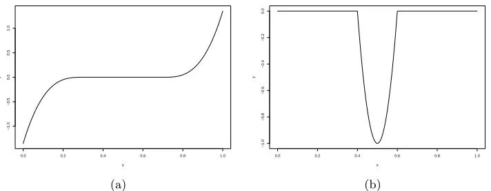
withϵ∼N(0,1). The true function a1(u) is defined as
a1(u) =
50(u−0.3)3 if 0≤u≤0.3 50(u−0.7)3 if 0.7≤u≤1
0 otherwise,
the plot of which is in panel (a) of Figure 2.1.
0.0 0.2 0.4 0.6 0.8 1.0
−1.0
−0.5
0.0
0.5
1.0
x
y
(a)
0.0 0.2 0.4 0.6 0.8 1.0
−1.0
−0.8
−0.6
−0.4
−0.2
0.0
x
y
(b)
Figure 2.1: Plots of a1(u) (left) anda2(u) (right) for simulation example.
The covariatesxi are generated iid fromN(0,4). The data pointsUiare chosen asnequally spaced design points on [0,1]. The sample sizes are varied to be n = 100,200,500 in the simulations. For estimation, we fix 501 equally spaced grid points on [0,1] and fit the penalized local polynomial regression on each point and get the estimates. We also run local polynomial regression on these grid points to make comparisons.
To examine the performance, we run 100 repetitions of Monte Carlo studies. As the zero region for the true function a1(u) is [0.3,0.7], define the correct zero coverage (correctzero) as
the proportion of region in [0.3,0.7] that is estimated as zero. The mean of correctzero in 100 repetitions will be reported. Moreover, we report the mean square error of the penalized local polynomial regression, which is defined as ∫01(ˆa1λ(u)−a1(u))2du. The mean square error of
the original local polynomial regression is also reported, which is∫01(ˆa1(u)−a1(u))2du. These
function. In addition, we generate an independent testing data set, which contains N = 501 groups of independent triples ( ˜Ui,xi,˜ Yi). The time points˜ Ui are chosen as 501 equally spaced points on [0,1]. Forxiandϵi in the testing data set, they are randomly generated from the same distributions as the training data set. Define the estimation error (EE) for the entire model as
EE =
∑N
i=1(˜xia1( ˜Ui)−x˜iea1( ˜Ui))2
N .
The estimation error of penalized local polynomial regression and local polynomial regression would be calculated, where we let ea1 = ˆa1λ and ea1 = ˆa1 respectively. The mean of the these
estimation errors will be reported, which are used to reflect the prediction error. The results for Example 1 are in Table 2.1.
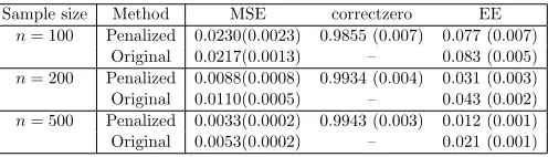
Table 2.1: Simulation results for the univariate case using penalized local polynomial regression and original local polynomial regression when sample size varies from n = 100,200,500. The entries in the table denotes mean square error (MSE) of the estimated function, the correct zero coverage (correctzero) and the estimation error (EE) for the entire model.
Sample size Method MSE correctzero EE
n= 100 Penalized 0.0230(0.0023) 0.9855 (0.007) 0.077 (0.007)
Original 0.0217(0.0013) – 0.083 (0.005)
n= 200 Penalized 0.0088(0.0008) 0.9934 (0.004) 0.031 (0.003)
Original 0.0110(0.0005) – 0.043 (0.002)
n= 500 Penalized 0.0033(0.0002) 0.9943 (0.003) 0.012 (0.001)
Original 0.0053(0.0002) – 0.021 (0.001)
2.5.2 Example 2
Next, we consider the bivariate case, where the data is simulated from the modelY =x1a1(u) +
x2a2(u) +ϵwith ϵ∼N(0,1). The first function a1(u) is the same function used in simulation
1. The second component functiona2(u) is defined as
a2(u) =
100((u−0.5)2−0.01) if 0.4≤u≤0.6
0 otherwise,
the plot of which is in panel (b) of Figure 2.1. It can be seen thata2(u) is not differentiable at
point 0.4 and 0.6.
For the design points Ui and the noiseϵi, the settings are the same as simulation 1. For the covariatesxi, we generate iid fromN(0,4I2), whereI2 is the 2×2 identity matrix. The sample
is fitted on 501 equally spaced grid points on [0,1]. An independent testing data set with size N = 501 is generated. The time points ˜Ui are still chosen as 501 equally spaced points on [0,1], and ˜xi1, ˜xi2 and ˜ϵi are generated the same as the training dataset. For the estimation error of the entire model, it is defined as
EE =
∑N
i=1(˜xi1a1( ˜Ui) + ˜xi2a2( ˜Ui)−x˜i1ea1( ˜Ui)−x˜i2ea2( ˜Ui))2
N .
The mean of MSE and correctzero for both two functions a1(·) and a2(·) will be reported.
The mean of the estimation errors for the entire model is also reported. All the results are summarized in Table 2.2.
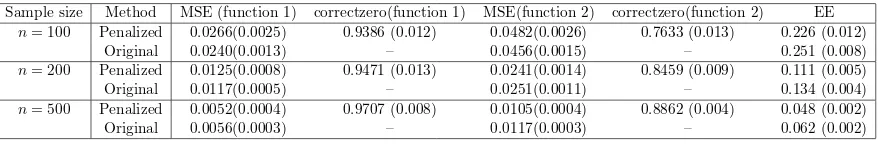
Table 2.2: Simulation results for the multivariate case using penalized local polynomial regres-sion and original local polynomial regresregres-sion when sample size varies from n = 100,200,500. The entries in the table denotes mean square error of the estimated functiona1(·) (MSE
(func-tion 1)) and a2(·) (MSE (function 2)), the correct zero coverage (correctzero) for a1(·)
(cor-rectzero(function 1)) anda2(·) (correctzero(function 2)), and the estimation error (EE) for the
entire model.
Sample size Method MSE (function 1) correctzero(function 1) MSE(function 2) correctzero(function 2) EE
n= 100 Penalized 0.0266(0.0025) 0.9386 (0.012) 0.0482(0.0026) 0.7633 (0.013) 0.226 (0.012)
Original 0.0240(0.0013) – 0.0456(0.0015) – 0.251 (0.008)
n= 200 Penalized 0.0125(0.0008) 0.9471 (0.013) 0.0241(0.0014) 0.8459 (0.009) 0.111 (0.005)
Original 0.0117(0.0005) – 0.0251(0.0011) – 0.134 (0.004)
n= 500 Penalized 0.0052(0.0004) 0.9707 (0.008) 0.0105(0.0004) 0.8862 (0.004) 0.048 (0.002)
Original 0.0056(0.0003) – 0.0117(0.0003) – 0.062 (0.002)
From these two simulations, we can see that our methods perform better than the original local polynomial regression in the sense that it gives smaller estimation error, which indicates better prediction. Meanwhile, we can estimate the zero regions of each component function quite well. When sample size increases, our method can capture the correct zero regions more accurately.
2.6
Real data application
oxides concentration parts per 10 million) and LSTAT (percentage of lower income status of the population), which might explain the variation of the housing value. The covariates CRIM, RM, TAX, NOX are denoted as x(2), . . . ,x(5), respectively. We setx(1) =1 to include the intercept term. We are interested in studying the association between the median value of the owner-occupied homes and these four covariates. As the distribution of LSTAT is asymmetric, similar as [14], the square root transformation is employed to make the resulting distribution symmetric. The histogram for the distribution of the√LSTAT is plotted in Figure 2.2. Specifically, we treat
histogram for lstat
originalx
Frequency
2 3 4 5 6
0
5
10
15
20
Figure 2.2: Histogram for √LST AT.
U =√LSTAT similarly as [14]. We construct the following model
Y =
5
∑
j=1
aj(U)x(j)+ϵ.
When dealing with the data, we center the response first. We also center and scale the covariates x(2), . . . ,x(5). As a1(·) is the intercept function, this term is not penalized. We only penalize
the functiona2(·), a3(·), a4(·), a5(·). We solve
min
a,b
n
∑
i=1
{Yi−x⊤i a−x⊤i b(Ui−u)}2(Kh(Ui−u)/Kh(0))
+m
5
∑
j=2
Pλ(
√
s2
where a = (a1, a2, a3, a4, a5)⊤ and b = (b1, b2, b3, b4, b5)⊤. The Epanechnikov kernel is
em-ployed, and the bandwidth (h = 1.23) is selected by the MSE tuning method. As we do not penalize the intercept term, we change the definition of degree of freedom used in tuning λby
∑5
j=2I(||βˆλj|| > 0) +
∑
j∈S ||βˆ
λj||
||βˆ
j||
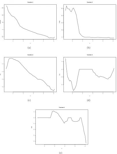
(dj −1). The estimated functions using our penalized local
polynomial regression (a1(·), a2(·), a3(·), a4(·), a5(·)) are plotted in panels (a)-(e) of Figure 2.3.
From Figure 2.3, we can see that the variable TAX has no effect on the response when U is between 2.6 to 4 and the variable NOX has no effect on the response when U is less than 2.6 or between 4.3 to 4.7.
We have also used the data to compare the prediction errors for both our penalized local polynomial regression and the original local polynomial regression. We randomly pick up 300 samples from the data as the training data and fit using both methods. After that, we use the remaining 206 data points as our test data, and we can get the prediction error given by
1
|S|
∑
2 3 4 5 6
−10
0
10
20
30
U
Intercept
Function 1
(a)
2 3 4 5 6
0
10
20
30
40
U
CRIM
Function 2
(b)
2 3 4 5 6
−2
0
2
4
U
RM
Function 3
(c)
2 3 4 5 6
−4
−2
0
2
U
T
AX
Function 4
(d)
2 3 4 5 6
−4
−3
−2
−1
0
1
U
NO
X
Function 5
(e)
Chapter 3
Fully efficient robust estimation,
outlier detection and variable
selection via penalized regression
3.1
Introduction
Outliers, which occur frequently in real data collection, are observations that deviate markedly from the rest of the observations. In the presence of outliers, likelihood-based inference can be unreliable, for example, the ordinary least squares (OLS) regression is very sensitive to outliers. To this end, outlier detection is critical in statistical learning because it can help to achieve robust statistical inference such as coefficient estimation, interval estimation and hypothesis testing. We consider the mean shift linear regression model yi =α+Xiβ+γi+ϵi, where Xi is ap dimensional predictor,β is apdimensional parameter, and γi is a mean shift parameter which is nonzero when the ith observation is an outlier. This model was previously used by [22, 42, 48], and represents the general notion that the response can be arbitrary.
In this article, we are interested in variable selection as well as robust coefficient estimation together with the task of outlier detection based on this mean shift model. A popular method for variable selection is the penalized regression method such as LASSO [50], SCAD [16] and adaptive LASSO [61]. In fact, these penalized regression methods cannot only be used for variable selection but outlier detection as well. For example, [42] used an L1 regression while [48] imposed a nonconvex penalty function on γi’s to avoid the trivial estimate ˆγi = yi and
ˆ
In the literature, asymptotic efficiency and breakdown point are two criteria to evaluate a robust regression technique. They represent the typical trade-off in efficiency for robust-ness. It is ideal to achieve full asymptotic efficiency compared to OLS while maintaining high breakdown point of 1/2. Typical robust regression methods do not enjoy these two properties simultaneously. The OLS, which is fully efficient, only has a breakdown point of 1/n, and hence even a single outlier can render the estimate arbitrarily bad. The M-estimates [33] also have a breakdown point of 1/n while Mallow Generalized M-estimates [40] can have a breakdown point of only 1/(p+ 1) [41, 10]. Moreover, neither of these two methods enjoys the full effi-ciency. There are several methods which enjoy high breakdown point of 1/2, such as the Least Median of Squares (LMS) estimates [25, 46], the Least Trimmed Squares (LTS) estimates [46], S-estimates [44], MM-estimates [56] and the Schweppe one-step Generalized M-estimates [7], however these methods are not fully efficient. There have been some methods introduced achiev-ing both properties, for example the Robust and Efficient Weighted Least Squares Estimators (REWLS) [23] and the generalized empirical likelihood method [2].
The proposed method achieves both full efficiency and high breakdown, while also perform-ing variable selection simultaneously. Specifically, our method is robust to outliers and enjoys a high breakdown point that can be as high as 1/2. Moreover, when there are no outliers, we show that applying our method is asymptotically equivalent to the penalized least squares for selection. In fact, if the regularization parameter is chosen appropriately, our estimator can enjoy full asymptotic efficiency under the gaussian distribution. Besides these properties, we also investigate the outlier detection consistency of our method, and show that under some regularity conditions, this method will correctly detect the outliers with probability tending to 1. In addition to these theoretical properties, we propose an efficient algorithm for our method, where the total number of unknown parameters, n+p, is larger than the sample size. The extended bayesian information criteria (EBIC) [4] is adopted to select the tuning parameters which control the outlier detection and variable selection respectively. Our method can also be extended to the high dimensional setting, where the dimension of the covariate p is diverging and much larger than the sample size. We show that the method still enjoys high breakdown even under the high dimension scenario.
3.2
Methodology
Denote y= (y1, . . . , yn)⊤, X= (X⊤1, . . . ,X⊤n)⊤, γ = (γ1, . . . , γn)⊤ and ϵ= (ϵ1, . . . , ϵn)⊤. Our model can be written as
where α is the intercept,1 is a n×1 vector with every element 1 and the error termϵi’s are i.i.d. withE(ϵi) = 0. These mean shift parametersγi’s serve as indicators of the outliers in the regression ofyi|Xi. If theith subject is an outlier,γi ̸= 0. Note that outliers may still occur in the covariate space, i.e. high leverage points, while having γi = 0, but we will show that these leverage points will not result in the breakdown of the estimator. We are interested in both outlier detection and variable selection for this model. To achieve these two goals, it is natural to devise a selection method via shrinkage. We impose penalties on γi’s to encourage them to shrink to zero and identify observations with nonzero γi’s as outliers. Meanwhile, we add penalties on the coefficient β to achieve variable selection. Specifically, we solve the following minimization problem
min
α,β,γQn(α,β,γ) = minα,β,γ||y−α1−Xβ−γ||
2 2+λn
p
∑
j=1
|βj|+µn n
∑
i=1 |γi|
|γie|, (3.1)
where eγi’s are obtained from the residuals of an initial robust regression fit. Here λn and µn are different regularization parameters controlling the variable selection and outlier detection respectively.
3.2.1 Robust Initial Estimator
It is interesting to note that we impose an adaptive penalty on γ which relies on the weight depending on an initial robust fit. The weight plays a similar role as the weight used in the adaptive LASSO problem [61], but it is based on the residuals rather than the parameter estimates. Various methods can be used for this initial step, for example LTS [46], LMS [25, 46], and MM-estimators [56], among others. The breakdown point of our method is at least as high as the breakdown point of the initial fit. In this article, we use the LTS method to obtain the initial robust estimates. We shall show that this will carry over to the high breakdown point of our estimator. Meanwhile, full efficiency and outlier detection consistency can be achieved by using this initial estimator. Theoretical properties of our estimators will be discussed in detail in Section 3. Denote ri = |yi−Xiβ|, the LTS method solves minβ
∑h
i=1r(2i), where r(i)’s are
the order statistics of ri with r(1) ≤ r(2) ≤ . . . ≤ r(n). The number of included residuals h
3.2.2 Algorithm
The optimization problem (4.2) is an L1 penalized problem and it can be easily transformed to a quadratic programming problem. A more efficient way is to use the Least Angle Regression algorithm (LARS) [11]. Define ρn= µn
λn, the optimization problem (4.2) becomes
min
α,β,γQn(α,β,γ) = minα,β,γ||y−α1−Xβ−γ||
2 2+λn{
p
∑
j=1
|βj|+ρn n
∑
i=1 |γi|
|γie|}.
For a fixed ρn, we can do reparameterization γ∗i = ρnγi
|eγi| and the problem becomes
min
α,β,γQn(α,β,γ) = minα,β,γ||y−α1−Xβ−Bγ
∗||2 2+λn{
p
∑
j=1 |βj|+
n
∑
i=1
|γ∗i|}, (3.2)
withB= diag(|eγ1|
ρn, . . . ,
|eγn|
ρn ) andγ
∗ = (γ∗
1, . . . , γn∗)⊤. Problem (3.2) is a typical LASSO problem, and can be solved easily by R package “lars”, which indeed gives the whole solution path of (2) as a function ofλn.
3.2.3 Tuning parameter selection
The optimization problem (4.2) involves tuning for two parametersλnand µn, which is equiv-alent to tuning λn and ρn together. Since the number of parameters is n+p and larger than the sample size, we use the extended BIC (EBIC)[4] due to its nice asymptotic properties for high dimensional problems. Suppose ˆβ and ˆγ are the estimates when the tuning parameters are set asλnand ρn. Let e2i = (yi−αˆ−X∗iβˆ−ˆγi)2, and define the residual sum of squares as RSS=∑ni=1e2i. The EBIC is defined as
EBIC = nlog(RSS/n) +k{logn+clog(n+p)},
changes. For high dimensional problems with the number of parameters exceeding the sample size, we will get a perfect fit if the df is large enough, which would make the EBIC very small as RSS goes to zero. This results in the wrong selection of λn because it tends to select theλn that gives a perfect fit. Consequently, we only search over the λn which leads to k ≤ ⌊0.5n⌋ because we assume that the number of outliers is less than half of the sample size.
3.3
Theoretical results
In this section, we discuss some theoretical properties. We investigate some asymptotic results for the estimators in the first two subsections, and we consider the high breakdown point in the last subsection. Without loss of generality, we only show the results for the case when there is no intercept. The results as well as the proofs for the case with an intercept follows in a similar manner.
3.3.1 Asymptotic theory when there are no outliers
We first consider the case when there are no outliers. We will show in this subsection that our methods can select important predictors consistently with probability tending to 1.
Since our method relies on the initial fit obtained from the least trimmed squares, more specifically, the residuals obtained from the least trimmed squares, we need some asymptotic results for the residuals, which are discussed in Lemma 1 and 2 in the Appendix. We start with the conditions that we need for our theorem and corollary.
Conditions (A)
(A1) For any 1≤j≤p,Xij’s follow an independent and identically distributed (iid) distribution withE(X2ij)<∞.
(A2) The errorϵi’s are iid with E(ϵ2ik)<∞ for somek >0. (A2’) The error ϵi’s follow an iid subgaussian distribution.
Condition (A1) is a mild condition imposing boundness on the second moment of the covariates. Condition (A2) assumes that the random error has a finite 2kth moment, which guarantees the polynomial tail bound. Condition (A2’) is a stronger condition than (A2), which indicates that the error has an exponential tail bound.
The design matrix is defined as
A=
(
X1,q Xq+1,p √nIn
)
and
C= 1 nA
⊤A=
C11 C12 C13
C21 C22 C23
C31 C32 C33
withC11= n1X⊤1,qX1,q,C21= n1X⊤q+1,pX1,q and C31= √1nX1,q. Our method is equivalent to solving
min
θ
1
2||y−Aθ||
2 2+λn
p
∑
j=1
|θj|+√nµn p+n
∑
j=p+1
|θj|/|γej−p|
Suppose a1 and a2 are two column vectors with same dimension, denote a1 ≤ a2 if the
inequality holds elementwise. Now we are ready to introduce the following conditions: Condition (B)
(B1) The strong irrepresentable condition: there exists a positive constant vector η such that
|C21C11−1sign(θ0(1))| ≤1−η.
There exists 0< d≤1 andM1, M2, M3>0 so that
(B2) 1nXj⊤Xj ≤M1 for any 1≤j≤p, whereXj denotes thejth column of X. (B3) α⊤C11α⊤≥M2 for any||α||= 1.
(B4) n1−2dminj=1,...,q|βj0| ≥M3.
Condition (B1) is introduced by [60] to guarantee the selection consistency for LASSO. Con-dition (B2) can be achieved by normalizing the covariates. ConCon-dition (B3) is trivial and only requires the smallest eigenvalue of the matrix C11 is nonzero. Condition (B4) quantifies the
smallest signal of the coefficient βj0, and we could identify the signal on the order of O(n
d−1
2 )
for some 0< d≤1.
Define a1 =s a2 if the signs of these two vectors are the same elementwise. We have the
following theorem:
Theorem 1 Under conditions (A1)(A2)(B), for λn = o(n(d+1)/2) and λn/√n → ∞, and
µnn−1/2k−d/2−1/2→ ∞, we haveP(ˆθ=sθ0)→1 as n→ ∞.
The condition can be relaxed if we assume the random errorϵi’s have subgaussian distribu-tion. We have the following corollary:
Corollary 1 Under conditions (A1)(A2’)(B), for λn=Cn1+d21 with a constant C, 0< d1< d
and µnn−1/2−d1/2(logn)−1/2 → ∞, we have P(ˆθ=sθ0)→1 asn→ ∞.
Remark: In fact, if we do not impose any penalty on β, i.e. λn = 0, which is the case of [48] by choosing the L-1 penalty, we have P(ˆγ = 0) → 1, which is equivalent to doing the least square regression. Thus, their estimator has full efficiency compared to the OLS. Even if we have the penalty on β as in our case, we can impose some conditions on λn such that the LASSO estimator has full efficiency compared to the OLS, though these conditions do not guarantee the selection consistency of LASSO estimator. The theoretical justification of the arguments here can be revealed in similar manner.
3.3.2 High breakdown point
Let the n×(p+ 1) matrix Z = (X,y) denote the sample, and Zem denotes the contaminated sample by replacing themdata points by arbitrary values. The finite sample breakdown point for the regression ˆβ is defined as
BP( ˆβ,Z) = min{m n : supZe
m
||β(ˆ Zm)e ||2 =∞},
where ˆβ(Zem) denotes the estimate of the regression parameter using the contaminated sample
e
Zm.
We assume the general position condition, which is standard in high breakdown point proofs. SupposeG is the set containing all good points (Xi, yi), for any p×1 vector v̸=0,{(Xi, yi) : (Xi, yi)∈G, and Xiv= 0} contains at mostp−1 points.
We first discuss the breakdown point proposed by [48]. Their method tries to solve
min
β,γ ||y−Xβ−γ||
2 2+
n
∑
i=1
Pµn(|γi|), (3.3)
where Pµn(·) is a nonconvex penalty. They have shown that their estimator is equivalent to
In contrast, our method would have high breakdown point of at least (n−h+ 1)/n, which is shown by the following theorem
Theorem 2 Suppose we use the least trimmed square with truncation number h as the initial estimator, under the general position condition, the breakdown point of our estimator satisfies thatBP( ˆβ,Z)≥min{(n−h+ 1)/n,⌊(n−p)/2⌋/n}.
Remark: It is well known that the LTS with truncation number h has a breakdown point of min{(n−h+ 1)/n,⌊(n−p)/2⌋/n}, see [45] for example. This theorem provides a lower bound of the breakdown point of the proposed method, which performs at least as well as the LTS initial estimator in terms of high breakdown point. However, we often choose h < n/2 so that the breakdown point can not exceed 0.5 since we aim for model to fit the majority of the data. In fact, if we do not impose any penalties on β, the estimator of our method would be a regression equivalent estimator in terms of β, which has an upper bound of the breakdown point of⌊(n−p)/2⌋+ 1.
This theorem reveals the importance of including adaptive weights while penalizing the mean shift parameter. Our estimator enjoys high breakdown by using the residuals of some robust initial fit with high breakdown such as the LTS method.
3.3.3 Outlier detection consistency
In this subsection, we consider the case when there are outliers in the conditional distribution of y|X, and show that we can identify these outliers consistently. We shall assume that the fraction of outliers in the data will remain nonzero as more data are collected, otherwise we are in the trivial case. Hence we have that sn = O(n). We will prove that our method can identify the outliers consistently under this scenario, i.e. identify the outlier as well as the normal observations with probability tending to 1. The same reparameterization η = γ/√n is done here. Without loss of generality, we assume the firstsn components η0(1) are outliers
while the remaining n−sn components η0(2) = 0 corresponding to the normal data points. With a little abuse of the notations from last subsection, we defineθ = (η(1)⊤,β⊤,η(2)⊤)⊤= (θ(1)⊤,θ(2)⊤,θ(3)⊤)⊤. DenoteXa:b as theath to bth row of the matrix X. The design matrix is defined as
A=
(
A1 A2
)
,
whereA1= ((√nIsn,0sn×(n−sn))⊤,X), A2 = (0(n−sn)×sn,
√
nIn−sn)⊤. Denote
C= 1 nA
⊤A=
(
C11 C12
C21 C22
with
C11=
(
Isn
1
√nX1:sn
1
√ nX⊤1:sn
1
nX⊤X
)
,
C21= (0(n−sn)×sn,
1
√
nXsn+1:n) and C22=In−sn.
The estimator is the solution to
min
θ
1
2||y−Aθ||
2 2+ √ nµn sn ∑ j=1
|θj|/|γej|+λn s∑n+p
j=sn+1
|θj|+√nµn p∑+n
j=p+sn+1
|θj|/|γej−p|
Noticing that sn =O(n), our problem is actually a weighted L-1 regression with the number of nonzero components on the order of O(n), so our problem is unlike the traditional high dimensional penalized problem for example [60], where they dealt with the case when the number of nonzero components is on the order ofO(na) witha <1.
Denote πn = mini=1,...,sn|γi0|. In addition to some of the conditions we state in the last
subsection, we need the following conditions: Condition (C)
(C1)πnn−1/2−1/2k→ ∞ asn→ ∞. (C1’) πnn−1/2(logn)−1/4 → ∞asn→ ∞.
(C2) The number of outlierssn< n−h,sn=O(n).
(C3) There exists M4>0 so that α⊤C11α⊤≥M4 for any||α||= 1.
Condition (C1) and (C1’) requires the minimum signal of the outliers diverges with the sample size. We show this assumption reasonable and necessary by the following simple case withyi =γi+ϵi, whereϵi ∼N(0,1) andγi =d >0 for 1≤i≤snandγi= 0 forsn+ 1≤i≤n. Hence, πn =d for this case. Since the support of the distribution is the entire real line, there cannot be a fixeddthat will define an “outlier” in this distribution. Hence it must be assumed that πn diverges sufficiently fast in order to distinguish the “outlier” from a random variable from the true distribution.
We state our main theorem of outlier detection consistency as follows
Theorem 3 Under conditions (A1)(A2)(B2)(C1)(C2)(C3), for µn = o(√π2n
n), µnn−
1/k → ∞, λn=o(
√
nπn) andλn=o(µnn1/2−1/2k), we haveP(ˆγ=sγ0)→1 as n→ ∞.
The conditions (C1) can be relaxed to (C1’) if we assume the error ϵi follows an iid sub-gaussian distribution, i.e. condition (A2’). We have the following corollary:
Corollary 2 Under conditions (A1)(A2’)(B2)(C1’)(C2)(C3), for µn = o(π
2 n
√ n),
√
logn/µn =
O(1), λn=o(√nπn) and λn=o(µn
√