Modeling Chilled-Water Storage System Components for Coupling to a Small Modular Reactor in a Nuclear Hybrid Energy System.

(1)

ABSTRACT

MISENHEIMER, COREY THOMAS. Modeling Chilled-Water Storage System Components for Coupling to a Small Modular Reactor in a Nuclear Hybrid Energy System. (Under the direction of Dr. Stephen D. Terry and Dr. Kevin Lyons).

The intermittency of wind and solar power puts strain on electric grids, often forcing carbon-based and nuclear sources of energy to operate in a load-follow mode. Operating nuclear reactors in a load-follow fashion is undesirable due to the associated thermal and mechanical stresses placed on the fuel and other reactor components. Various Thermal Energy Storage (TES) elements and ancillary energy applications can be coupled to nuclear (or renewable) power sources to help absorb grid instabilities caused by daily electric demand changes and renewable intermittency, thereby forming the basis of a candidate Nuclear Hybrid Energy System (NHES).

During the warmer months of the year in many parts of the country, facility air-conditioning loads are significant contributors to the increase in the daily peak electric demand. Previous research demonstrated that a stratified chilled-water storage tank can displace peak cooling loads to off-peak hours. Based on these findings, the objective of this work is to evaluate the prospect of using a stratified chilled-water storage tank as a potential TES reservoir for a nuclear reactor in a NHES. This is accomplished by developing time-dependent models of chilled-water system components, including absorption chillers, cooling towers, a storage tank, and facility cooling loads appropriate for a large office space or college campus, as a callable FORTRAN subroutine. The resulting TES model is coupled to a high-fidelity mPower-sized Small Modular Reactor (SMR) Simulator, with the goal of utilizing excess reactor capacity to operate several sizable chillers in order to keep reactor power constant.

(2)

model, a low-fidelity absorption chiller model is formulated and calibrated to mimic the behavior of the high-fidelity model.

Stratified chilled-water storage tank performance is characterized using Computational Fluid Dynamics (CFD). The geometry employed in the CFD model represents a 5-million-gallon storage tank currently in use at a North Carolina college campus. Simulation results reveal the laminar numerical model most closely aligns with actual tank charging and discharging data. A subsequent parametric study corroborates storage tank behavior documented throughout literature and industry.

Two absorption chiller configurations are considered. The first involves bypassing low-pressure steam from the low-low-pressure turbine to absorption chillers during periods of excess reactor capacity in order to keep reactor power constant. Simulation results show steam conditions downstream of the turbine control valves are a strong function of turbine load, and absorption chiller performance is hindered by reduced turbine impulse pressures at reduced turbine demands.

A more suitable configuration entails integrating the absorption chillers into a flash vessel system that is thermally coupled to a sensible heat storage system. The sensible heat storage system is able to maintain reactor thermal output constant at 100% and match turbine output with several different electric demand profiles. High-pressure condensate in the sensible heat storage system is dropped across a let-down orifice and flashed in an ideal separator.

Generated steam is sent to a bank of absorption chillers. Simulation results show enough steam is available during periods of reduced turbine demand to power four large absorption chillers to charge a 5-million-gallon stratified chilled-water storage tank, which is used to offset cooling loads in an adjacent facility. The coupled TES systems operating in

(3)

(4)

Modeling Chilled-Water Storage System Components for Coupling to a Small Modular Reactor in a Nuclear Hybrid Energy System

by

Corey Thomas Misenheimer

A dissertation submitted to the Graduate Faculty of North Carolina State University

in partial fulfillment of the requirements for the Degree of

Doctor of Philosophy

Mechanical Engineering

Raleigh, North Carolina 2017

APPROVED BY:

_______________________________ _______________________________

Dr. Stephen D. Terry Dr. Kevin Lyons

Co-Chair of Advisory Committee Co-Chair of Advisory Committee

_______________________________ _______________________________ Dr. J. Michael Doster Dr. Peter Corson

(5)

DEDICATION

(6)

BIOGRAPHY

Corey Thomas Misenheimer was the first child born to Carl and Laura Misenheimer in Charlotte, NC. As a child, he played nearly every imaginable sport, eventually gravitating towards soccer and playing competitively until the age of 20.

Corey enrolled at NC State University in 2009, though there was never really any doubt being a child of two NC State alumni. At NC State, he matriculated into the Mechanical Engineering degree program, where he developed a keen interest for heat transfer,

(7)

ACKNOWLEDGEMENTS

First and foremost, I would like to thank my parents. Their support for me throughout this eight-year endeavor has been unwavering. They provided me with every imaginable tool necessary to succeed, as a student and as an individual.

I would like to express gratitude to my adviser, Dr. Stephen D. Terry. In 2013, Dr. Terry offered me the opportunity to investigate Nuclear Hybrid Energy Systems under his guidance. His years of experience from working in and now leading the Industrial

Assessment Center (IAC) at NC State have been invaluable during my four years in graduate school. His door is always open, and I could always count on him being in his office before 7:00 am.

I would also like to thank Dr. Doster from the Nuclear Engineering Department at NC State for his guidance on this project, as well as letting me use his SMR Simulator. His expertise in thermal hydraulics and SMR model added an additional, unique layer to this project. Much recognition must be given to his graduate student, Konor Frick, as well. He developed the flash vessel model, wrote the associated documentation, and provided me with various input files to run numerous other interesting simulations that form the basis of this

dissertation. Konor has been my primary contact throughout this project for nuclear-related inquiries.

I am thankful for funding through the INL Laboratory Directed Research & Development (LDRD) Program under DOE Idaho Operations Contract No. DE-AC07-05ID14517. Of course, I am grateful Dr. Bragg-Sitton afforded me the opportunity to work on this project. She has provided feedback over the course of this project on papers and presentations, and has overall been fantastic to work with.

(8)

Current and former members of the IAC here at NC State must be acknowledged, as we shared lab space. Several of them, including James Turner, Taylor Atkins, Gopal Chaudhary, John Nickels, Daniel Paprocki, Jackson Wooten, Tucker Daniels, and Harrison Kesling, offered valuable consulting over the years, free of charge.

(9)

TABLE OF CONTENTS

LIST OF TABLES ... x

LIST OF FIGURES ... xi

NOMENCLATURE ... xviii

Subscripts ... xxii

Chapter 1 Introduction ... 1

1.1 Ancillary Energy Applications and TES Methods ... 7

1.1.1 Ancillary Energy Applications ... 7

1.1.1.1 Water Desalination ... 8

1.1.1.2 Oil Refining ... 8

1.1.1.3 Hydrogen Production ... 10

1.1.2 TES Methods ... 11

1.1.2.1 Steam Accumulation... 11

1.1.2.2 Sensible Heat Storage ... 12

1.1.2.3 Chilled-Water Storage ... 13

1.2 Project Overview ... 14

Chapter 2 Storage Element Analysis ... 16

2.1 Previous Work ... 16

2.2 Numerical Model... 20

2.2.1 Tank Overview... 20

2.2.2 Geometry... 23

2.2.3 Meshing... 25

(10)

2.2.4.1 Laminar Governing Equations ... 28

2.2.4.2 Turbulent Governing Equations ... 29

2.2.5 Field Data ... 34

2.2.6 Performance Metrics ... 36

2.2.7 Results and Discussion ... 39

2.2.7.1 Tank Charging ... 41

2.2.7.2 Tank Discharging ... 48

2.2.8 Parametric Study ... 50

2.2.8.1 Charging Parametric Study ... 50

2.2.8.2 Discharging Parametric Study ... 54

2.2.9 Comments on Potential Sources of Error... 58

Chapter 3 Electric Chiller Modeling ... 61

3.1 System Overview ... 61

3.2 Electric Chiller Model ... 63

3.3 Cooling Tower Model ... 64

3.4 Stratified Chilled-Water Storage Tank Analysis ... 68

3.5 Model Description ... 72

3.6 Results and Discussion ... 74

3.7 Conclusions ... 81

Chapter 4 High-Fidelity Dynamic Absorption Chiller Model... 82

4.1 Introduction ... 82

4.2 Dynamic Model Description ... 86

(11)

4.2.2 Absorber ... 89

4.2.3 Generator... 90

4.2.4 Intermediate Heat Exchanger ... 90

4.2.5 Other Devices... 91

4.3 Definition of Parameters ... 92

4.3.1 Methods... 92

4.3.2 Generator... 95

4.3.3 Solution Strategy ... 99

4.3.3.1 Generator Solution Strategy ... 100

4.3.3.2 Overall Solution Strategy ... 103

4.4.1 Steady-State Trends ... 108

4.4.2 Transient Results ... 116

4.4.3 Comments on Numerical Scheme ... 123

Chapter 5 Low-Fidelity Dynamic Absorption Chiller Model ... 125

5.1 Formulation ... 125

5.2 Calibration ... 130

Chapter 6 Chilled-Water Storage Integration with SMR ... 138

6.1 SMR Simulator ... 138

6.1.1 SMR Simulator Overview... 138

(12)

6.1.3 Absorption Chiller Integration with SMR Simulator... 143

Chapter 7 Chilled-Water Storage Integration with Sensible TES System ... 152

7.1 Sensible Heat Storage System Overview ... 152

7.2 Absorption Chiller and Chilled-Water Storage Integration with TES System ... 153

7.2.1 Flash Vessel System Overview ... 154

7.2.2 Additional Absorption Chiller Model Requirements ... 156

7.3.1 Sensible Heat Storage System in Charging-Only Mode ... 162

7.3.1.1 Typical Summer Day ... 162

7.3.1.2 Typical Summer Day with High Renewable (Solar) Penetration... 166

7.3.2 Sensible Heat Storage System Charging and Discharging ... 171

7.3.2.1 Typical Summer Day ... 171

7.3.2.2 Typical Summer Day with High Renewable (Solar) Penetration... 175

Chapter 8 Conclusions and Future Work ... 180

Funding ... 183

(13)

LIST OF TABLES

Table 2.1: Supplemental Stratified Chilled-Water Storage Tank Information ... 23

Table 2.2: Dimensions for Both Tank Geometries ... 24

Table 2.3: Boundary Conditions for Both Tank Geometries ... 25

Table 2.4: Meshing Characteristics for Both Tank Geometries ... 25

Table 2.5: Water Properties Used in CFD Simulations ... 28

Table 2.6: Charging Simulation Settings ... 40

Table 2.7: Discharging Simulation Settings ... 40

Table 3.1: Simulation Parameters ... 75

Table 4.1: Nominal Absorption Chiller Parameters ... 107

Table 4.2: Steady-State Trend Summary ... 111

Table 4.3: Transient Simulation Parameters ... 118

Table 5.1: Heat Exchanger Mass Amplification Factors ... 132

Table 6.1: Nominal SMR System Parameters ... 140

(14)

LIST OF FIGURES

Figure 1.1: NERC regions and approximate BA locations, as of October 1, 2015 [2]... 2

Figure 1.2: Normalized demand profile in the Carolinas on a typical summer day [5] ... 3

Figure 1.3: “Duck Curve” from substantial renewable energy (solar PV) integration in California [15] ... 5

Figure 1.4: Proposed baseload installation comprised of five NuScale modules [17] ... 6

Figure 1.5: Example architecture for a tightly coupled NHES, as proposed by Idaho National Laboratory (INL) [20] ... 7

Figure 1.6: Fractional distillation column [23] ... 9

Figure 1.7: Proposed steam accumulator Rankine cycle configuration [20] ... 12

Figure 1.8: Example thermocline during stratified chilled-water storage tank charging procedure... 14

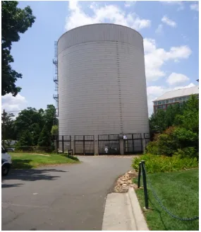
Figure 2.1: Stratified chilled-water storage tank in Chapel Hill, NC ... 21

Figure 2.2: Bottom hexagonal radial diffuser ... 21

Figure 2.3: Top hexagonal radial diffuser... 22

Figure 2.4: Tank geometry for turbulent regime (a) and laminar regime (b) ... 24

Figure 2.5: Generated mesh for turbulent regime geometry (left) and laminar regime geometry (right) ... 26

Figure 2.6: Meausured tank charging flow rate versus approximated ... 35

Figure 2.7: Measured tank inlet chilled-water temperature versus approximated ... 35

Figure 2.8: Measured tank discharging flow rate versus approximated ... 36

Figure 2.9: Measured tank inlet warm-water temperature versus approximated ... 36

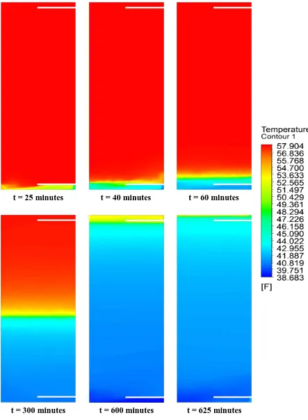
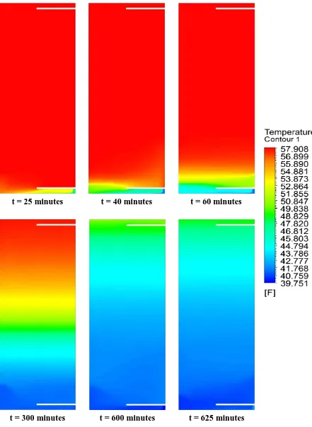
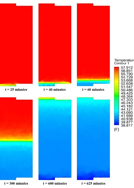
Figure 2.10: Temperature contour plots at various points in time during tank charging process using realizable k – ε turbulent model ... 44

Figure 2.11: Temperature contour plots at various points in time during tank charging process using SST k – ω turbulent model ... 45

(15)

Figure 2.13: Thermocline propagation using realizable k – ε turbulent model ... 47

Figure 2.14: Thermocline propagation using SST k – ω turbulent model ... 47

Figure 2.15: Thermocline propagation using laminar model... 47

Figure 2.16: Measured tank outlet temperature versus simulated ... 47

Figure 2.17: Temperature contour plots at various points in time during tank discharging process using laminar model ... 49

Figure 2.18: Thermocline propagation using laminar model... 50

Figure 2.19: Measured tank outlet temperature versus simulated ... 50

Figure 2.20: CWL versus Θlim at varying charging flow rates for initial temperature difference of 9oF ... 53

Figure 2.21: CWL versus Θlim at varying charging flow rates for initial temperature difference of 12oF ... 53

Figure 2.22: CWL versus Θlim at varying charging flow rates for intial temperature difference of 15oF ... 53

Figure 2.23: CWL versus charging flow rates at varying temperature differences for a Θlim of 0.70... 54

Figure 2.24: CWL versus Θlim at varying discharging flow rates for intial temperature difference of 9o_{F ... 57}

Figure 2.25: CWL versus Θlim at varying discharging flow rates for intial temperature difference of 12o_{F ... 57}

Figure 2.26: CWL versus Θlim at varying discharging flow rates for intial temperature difference of 15oF ... 57

Figure 2.27: CWL versus discharging flow rates at varying temperature differences for a Θlim of 0.30 ... 58

Figure 3.1: Modeled TES system... 62

Figure 3.2: Chiller efficiency curves ... 64

Figure 3.3: Cooling tower characteristic curve for 625 nominal ton counterflow cooling tower [55] ... 67

(16)

Figure 3.5: Required chiller input power ... 76

Figure 3.6: Stratified chilled-water storage tank level ... 76

Figure 3.7: Facility power ... 76

Figure 3.8: CWL ... 76

Figure 3.9: Required chiller input power ... 79

Figure 3.11: Facility power ... 80

Figure 3.12: CWL ... 80

Figure 4.1: Single effect, LiBr absorption chiller model [77] ... 87

Figure 4.2: Graphical generator solution strategy... 102

Figure 4.3: Pressure and quality along generator tube bundle ... 108

Figure 4.4: Steam temperature, tube wall temperature, and quality along generator tube bundle ... 109

Figure 4.5: Quality along generator tube bundle versus inlet steam pressure ... 111

Figure 4.6: Quality along generator tube bundle versus steam mass flow rate ... 111

Figure 4.7: Quality along generator tube bundle versus cooling tower return water temperature ... 113

Figure 4.8: Absorption chiller percent design energy input versus chiller capacity [78] ... 113

Figure 4.9: Quality along generator tube bundle versus chilled-water flow rate ... 116

Figure 4.10: Absorption chiller capacity versus chilled-water temperature leaving evaporator [78] ... 116

Figure 4.11: Schematic of thermal system for transient simulation ... 117

Figure 4.12: Generator tube-side inlet steam pressure and outlet pressure ... 119

Figure 4.13: Overall steam condensation length ... 119

Figure 4.14: Condensate return temperature ... 119

Figure 4.15: Internal refrigerant mass flow rates ... 120

Figure 4.16: Internal water-LiBr solution mass flow rates ... 120

Figure 4.17: Average internal shell-side heat exchanger temperatures ... 120

(17)

Figure 4.19: LiBr mass fractions ... 121

Figure 4.20: Heat exchanger masses ... 121

Figure 4.21: Absorption chiller capacity ... 122

Figure 4.22: Absorption chiller COP ... 122

Figure 5.1: Low-fidelity absorption chiller model diagram... 128

Figure 5.2: Average shell-side temperature model response to step increase in steam mass flow rate and pressure ... 131

Figure 5.3: Tube-side temperature model response to step increase in steam mass flow rate and pressure ... 131

Figure 5.4: LiBr mass fraction model response to step increase in steam mass flow rate and pressure ... 131

Figure 5.5: Condensate return temperature model response to step increase in steam mass flow rate and pressure ... 131

Figure 5.6: Average shell-side temperature model response to step increase in steam mass flow rate and pressure (T13 = constant) ... 133

Figure 5.7: Tube-side temperature model response to step increase in steam mass flow rate and pressure (T13 = constant) ... 133

Figure 5.8: LiBr mass fraction model response to step increase in steam mass flow rate and pressure (T13 = constant) ... 133

Figure 5.9: Condensate return temperature model response to step increase in steam mass flow rate and pressure (T13 = constant) ... 133

Figure 5.10: Average shell-side temperature model response to step increase in steam mass flow rate and pressure ... 134

Figure 5.11: Tube-side temperature model response to step increase in steam mass flow rate and pressure ... 134

Figure 5.12: LiBr mass fraction model response to step increase in steam mass flow rate and pressure ... 134

(18)

Figure 5.14: Average shell-side temperature model response to gradual sinusoidal change in

steam mass flow rate and pressure ... 135

Figure 5.15: Tube-side temperature model response to gradual sinusoidal change in steam mass flow rate and pressure ... 135

Figure 5.16: LiBr mass fraction model response to gradual sinusoidal change in steam mass flow rate and pressure ... 135

Figure 5.17: Condensate return temperature model response to gradual sinusoidal change in steam mass flow rate and pressure ... 135

Figure 6.1: SMR Simulator [93] ... 139

Figure 6.2: Turbine output and electric demand ... 141

Figure 6.3: Reactor thermal power ... 141

Figure 6.4: Primary coolant temperatures ... 141

Figure 6.5: Control rod position... 141

Figure 6.6: OTSG and turbine impulse pressure ... 142

Figure 6.7: OTSG dryout location ... 142

Figure 6.8: Absorption chiller SMR integration ... 144

Figure 6.9: Facility cooling demand profile ... 145

Figure 6.10: Ambient dry bulb and wet bulb temperature profiles... 145

Figure 6.11: Discharging CWL curves for Θlim = 0.2 ... 146

Figure 6.12: Turbine output and electric demand ... 146

Figure 6.13: Reactor thermal power ... 146

Figure 6.14: Primary coolant temperatures ... 146

Figure 6.15: Control rod position... 147

Figure 6.16: OTSG and turbine impulse pressure ... 147

Figure 6.17: OTSG dryout location ... 147

Figure 6.20: Chilled-water temperature ... 148

(19)

Figure 6.22: Bypass steam mass flow rate ... 148

Figure 6.23: Chilled-water temperature versus percent turbine output ... 151

Figure 6.24: Chiller capacity versus percent turbine output ... 151

Figure 7.1: Sensible heat storage system, charging mode [95] ... 153

Figure 7.2: Flash vessel system configuration for chilled-water production via absorption chillers [96] ... 154

Figure 7.3: Absorption chiller integration with flash vessel system for chilled-water production and storage ... 155

Figure 7.4: Quality along generator tube bundle ... 159

Figure 7.5: Steam temperature along generator tube bundle ... 159

Figure 7.6: Steam pressure along generator tube bundle ... 159

Figure 7.7: Axial tube wall temperature gradient ... 159

Figure 7.8: Quality along generator tube bundle versus inlet steam superheat ... 161

Figure 7.9: Electric demand and turbine output [95] ... 163

Figure 7.10: Reactor thermal power [95] ... 163

Figure 7.11: Flash vessel system mass flow rates... 164

Figure 7.12: Flash vessel system pressures... 164

Figure 7.13: Flash vessel condensate level ... 164

Figure 7.16: Chilled-water system temperatures ... 165

Figure 7.17: Turbine demand for typical summer day with 40 MWe solar PV [99] ... 167

(20)

(21)

NOMENCLATURE

Latin Variables

A Area (ft2)

a Thermal diffusivity (ft2/hr)

act Area of air-water interface (ft2/ft3)

a1, a2 Integration limits ACV Auxiliary control valve

AF Mass amplification factor (--)

ASHRAE American Society of Heating, Refrigerating, and Air-Conditioning Engineers

b1, b2 Constants in LiBr state equation (--) BA Balancing authority

C Correction factor (--)

Cd Discharge coefficient (--)

Cint Integrated capacity (--)

Clost Lost capacity (--)

Cmax Maximum capacity (--)

cp Specific heat (BTU/lbm-oF)

CR Heat capacity ratio (--)

C1 Variable in realizable k – ε RANS equations (--)

C2 Constant in realizable k – ε RANS equations (--)

c1, c2 Constants in condensation HTC equations (--)

C1ε Constant in realizable k – ε RANS equations (--)

C3ε Variable used to calculate buoyancy effects on turbulence dissipation rate in realizable k – ε RANS equations (--)

Cμ Variable used to calculate turbulent viscosity in realizable k – ε RANS equations (--)

CFD Computational fluid dynamics CHP Combined heat and power

CLTD Cooling load temperature difference (o_F)

COP Coefficient of performance (--)

CV Control volume CWL Chilled-water lost (%)

D Diameter (ft)

d Thickness (ft)

Dω Cross-diffusion term (lbm/hr2-ft3) DNS Direct numerical simulation

E Total energy (BTU)

E1 Constant in two-phase flow multiplier equation (--)

f Function (--)

F1 Constant in two-phase flow multiplier equation (--)

(22)

FOM Figure of merit (--) Fr Froude number (--)

Frso Froude transition number (--) G Mass flux (ft/hr-m2)

g Gravity (ft/hr2)

gc Gravitational constant (lbm-ft/lbf-hr2)

Gb Turbulence kinetic energy generation from buoyancy (lbm/hr3-ft)

Gk Turbulence kinetic energy generation via mean velocity gradients (lbm/hr3-ft)

Gω Specific turbulence dissipation rate generation (lbm/hr2-ft3) Ga Galileo number (--)

GHG Greenhouse gas

H Height (ft)

h Specific enthalpy (BTU/lbm)

H1 Constant in two-phase flow multiplier equation (--) HTC Heat transfer coefficient

HVAC Heating, ventilation, and air-conditioning IHX Intermediate heat exchanger

INL Idaho National Laboratory

J Jacobian Matrix (--) Ja Jakob number (--)

Kct Overall unit surface conductance for energy transfer (lbm/hr)

k Turbulence kinetic energy (ft2/hr2)

L Length (ft)

LCV Level control valve LES Large eddy simulation LiBr Lithium bromide

LM Latitude and monthly correction factor (oF) LMTD Log-mean temperature difference

M Mass (lbm)

m Mass flow rate (lbm/hr) MED Multi-effect distillation MSF Multi-stage flash distillation

N Number of (--)

n Number of tubes (tubes)

NERC North American Electric Reliability Corporation NHES Nuclear Hybrid Energy System

NR Average number of tubes per row (tubes/row) NTU Number of transfer units (--)

Nu Nusselt number (--)

O Denotes order of accuracy of numerical approximation (--) OTSG Once through steam generator

P Pressure (psia)

(23)

Pr Prandtl number (--)

Prt Turbulent Prandtl number for energy (--)

PV Photovoltaic

PWR Pressurized water reactor

Q Heat transfer rate (BTU/hr)

q Heat flux (BTU/hr-ft2₎ R Radius (ft)

r Radial direction or distance (ft)

fo

R _{Fouling thermal resistance (ft}2_-o_F-hr/BTU) Rair Ideal gas constant for air (ft-lbf/lbm-R) Re Reynolds number (--)

Rels Superficial Reynolds numbers (--)

RANS Reynolds-averaged Navier-Stokes RO Reverse osmosis

S Modulus of mean-rate-of-strain tensor (1/hr)

Sh Source term in heat transport equation (BTU-lbm/ft3-hr)

Sk Source term for turbulence kinetic energy (lbm/hr3-ft)

Sε Source term for turbulence dissipation rate (lbm/hr4-ft)

Sω Source term for specific turbulence dissipation rate (lbm/hr2-ft3) SCV Steam control valve

SMR Small modular reactor

T Temperature (o_F) t Time (hr)

TBV Turbine bypass valve TCV Turbine control valve TES Thermal energy storage TMY Typical meteorological year

U Internal Energy (BTU)

u Specific internal energy (BTU/lbm)

UA Overall heat transfer coefficient (BTU/hr-oF) UDF User defined function

V Volume (ft3₎ v Velocity (ft/hr)

V Volumetric flow rate (gpm)

Vct Active cooling tower volume (ft3/ft2) VFD Variable frequency drive

w Specific humidity (--) We Weber number (--)

X Lithium bromide mass fraction (--)

x General Cartesian direction (--)

xst Quality (--)

(24)

y Fluid level in heat exchanger (ft)

Yk Dissipation of turbulence kinetic energy (lbm/hr3-ft)

YM Dilalation dissipation (lbm/hr3-ft)

Yω Dissipation of specific turbulence dissipation rate (lbm/hr2-ft3)

Y+ Dimensionless wall distance (--)

z Axial distance (ft) Greek Variables

 Heat transfer coefficient (BTU/hr-ft2-oF)  Coefficient of thermal expansion (1/o_F)

 Difference

ij

 Kronecker delta function (--)  Turbulence dissipation rate (ft2/hr3)

ct

 Effectiveness of cooling tower (--)

IHX

 Effectiveness of IHX in absorption chiller (--)  Scalar quantity (--)

2 lo

 Two-phase flow multiplier (--)

o

 Film mass flow rate (lbm/hr-ft) k

 Effective diffusivity of turbulence kinetic energy (lbm/ft-hr) 

 Effective diffusivity of specific turbulence dissipation rate (lbm/ft-hr)

 _{Exponential cooling tower performance coefficient (--)}



Exponential cooling tower performance coefficient (--)

 _{Dynamic viscosity (lbm/ft-hr)}

t

 Turbulent viscosity (lbm/ft-hr)  Kinematic viscosity (ft2/hr)

 _{Thermal conductivity (BTU/hr-ft-}o_F)

Θ Dimensionless temperature (--)

strat

 Angle from top of tube to condensate level in bottom of tube (Ra)

 _{Density (lbm/ft}3₎

h

 Two-phase density (lbm/ft3)  Void fraction (--)

k

 Turbulent Prandtl number for turbulence kinetic energy (--)



 Turbulent Prandtl number for turbulence dissipation rate (--)  Specific turbulence dissipation rate (1/hr)

(25)

Subscripts

abs Absorber acc Acceleration actual Actual

air Air

amb Ambient atm Atmospheric ave Average base Uncorrected bypass Bypass calc Calculated ch Chilled water char Tank charging

chiller Denotes steam conditions downstream of chiller valve in flash vessel system CL Cold leg

cold Cold water in storage tank con Condenser

corrected Corrected ct Cooling tower db Dry Bulb dif Diffuser

dischar Tank discharging eva Evaporator f Friction

fi Film

FV Flash vessel gen Generator HF High-fidelity HL Hot leg

i Inside

impulse2 Denotes steam conditions downstream bank of PCVs in flash vessel system in Inlet

int Integrated

i, j, k Denotes general cartesian direction k Denotes iteration

l Liquid

LF Low-fidelity lim Limiting

lm Log-mean

lo Liquid only lost Lost

(26)

net Net

no Nodes

nom Nominal

o Outside

out Outlet

pan Refrigerant pan

r Radial

recirc Recirculation ref Refrigerant

return Warm water returned from cooling load tank Flow rate through storage tank

sat Saturated sh Superheat small Small sol Solution

st Steam

strong Concentrated water-LiBr solution mixture

t Tube

tot Total

v Vapor

vapor Water vapor properties in ambient air vo Vapor only

w Wall

warm Warm water in storage tank wb Wet bulb

weak Dilute water-LiBr solution mixture x Cross-sectional

z Axial

0 Reference

(27)

Chapter 1 Introduction

The widespread generation and transmission of electricity is a fundamental identifier of a modern developed country. Through a country’s electric grid, residential and industrial consumers are able to utilize electrical power to run appliances, condition homes and other spaces, and energize a multitude of technological devices. Average consumers do not allocate much thought to pondering the origin of their electricity; yet, the availability of electricity is never questioned when a light switch is turned on or a phone is plugged-in, save for outages during inclement weather. In reality, electricity in the United States originates at various conventional power plants and renewable energy sources dispersed across the

country. Electricity is subsequently sent to substations for either local distribution or long-distance transmission. Much like temperature differences induce heat transfer, voltage differences prompt electrical current. At these substations, voltage can be increased (stepped-up) for more efficient travel through long-distance high-voltage power lines, or voltage can be decreased (stepped-down) for the transmission through distribution lines to nearby consumers. This large interconnection of suppliers and consumers across vast regions comprises the electric grid, sometimes simply referred to as the “grid”.

The United States power system is divided into three primary interconnections, or grids: The Eastern Interconnection, The Western Interconnection, and the Electric Reliability Council of Texas. The interconnections can be further subdivided into regional entities, regional

transmission organizations (RTOs), and independent system operators (ISOs). Balancing authorities (BAs) manage electric grid operations at the regional level. Per the North

(28)

Figure 1.1: NERC regions and approximate BA locations, as of October 1, 2015 [2] A lack of economical large-scale electrical storage elements on the electric grid means that BAs have to match the supply and demand of electricity down to second-by-second

(29)

afternoon hours due to large thermal masses of buildings put further strain on utilities during warmer months. To account for these abnormally high loads, fast peaking generators can be brought online.

Figure 1.2: Normalized demand profile in the Carolinas on a typical summer day [5] As previously mentioned, gas-fired plants are more proficient at load-following compared to coal-fired and nuclear plants, making them ideal candidates for satisfying intermediate and peak loads illustrated in Figure 1.2. Recent revolutionary hydraulic fracturing techniques, such as horizontal drilling, have resulted in a natural gas market explosion and a subsequent plunge in natural gas prices. Electricity generation via natural gas combustion dethroned coal as the largest power source in 2015 for the first time in history in the United States [6]. Despite the U.S. Energy Information Administration’s (EIA) short term forecasted price increases for natural gas, in 2016 and early 2017 the Federal Energy Regulatory Committee (FERC) awarded certifications for natural gas pipeline and pipeline expansions to

accommodate an additional estimated 24.6 billion cubic feet of natural gas per day (Bcf/d) [7], [8]. The combustion of natural gas for power generating purposes also offers a cleaner

Peaking

Intermediate

(30)

carbon atom and four hydrogen atoms per molecule. Coal’s higher carbon-to-hydrogen ratio results in more carbon dioxide emissions, a greenhouse gas (GHG), during oxidation

compared to natural gas. Moreover, coal combustion has been found to create corrosive sulfuric acid, hazardous fine particulates, and coal ash with various toxic heavy metals and trace amounts of radioactive nuclides [9].

At the same time, mounting evidence from the scientific community linking rising global temperatures to atmospheric carbon dioxide levels has made hydrocarbon combustion for power generation purposes less desirable. In a paper published by Cook et al. [10], the authors examined 11,944 climate change related peer reviewed papers. They found that of the paper authors that took a clear explicit or implicit position on human induced global warming, over 98% of the authors believe human related activities are to blame for rising global temperatures [10]. Tol [11] offered a sharp rebuttal, pointing out that the study performed by Cook et al. essentially disregarded the papers that took no discernable position on global warming. This in turn prompted another response by Cook et al. [12], clarifying and fortifying their position that a majority of climate scientists believe humans are to blame for rising global temperatures. It is clear that global warming is still a hotly debated topic. However, rising atmospheric carbon dioxide levels are undeniable per data from the National Aeronautics and Space Administration (NASA) and the National Oceanic and Atmospheric Administration (NOAA) [13]. Rising atmospheric carbon dioxide levels combined with the gas’s natural propensity to absorb and emit wavelengths in the infrared spectrum have rendered the small fraction of climate-change-denying scientists’ position all but invalid. While natural gas combustion results in fewer carbon dioxide emissions than the burning of coal, the scientific community and climate activists continue to pressure the government and utilities to further curb atmospheric GHG emissions.

(31)

wind electric grid implementation in several states. The result has been a rapid buildout of wind technology and solar PV plants in some regions of the United States. For instance, North Carolina installed 1,140 MW of solar PV capacity in 2015 after becoming the first state in the southeast to adopt a renewable energy portfolio standard [14]. As of 2017, North Carolina has the second most installed solar PV capacity in the United States behind only California [14]. However, renewable energy technology grid integration presents a new set of challenges, specifically, intermittent, non-dispatchable energy. Put simply, solar PV plants do not produce power at night and experience large plant capacity reductions during times of cloud cover, while wind farms rely on fluctuating air movement. Sudden weather changes make matching electricity supply and demand difficult for BAs. This problem becomes more pronounced with increased renewable energy technology penetration into the electric grid, as shown in Figure 1.3 [15].

Figure 1.3: “Duck Curve” from substantial renewable energy (solar PV) integration in California [15]

(32)

that can be constructed at a single location and deployed to various sites. In addition to providing reliable power with no carbon emissions, these Small Modular Reactors (SMRs) offer increased site compatibility, advanced passive safety systems for the removal of decay heat, a reduction in primary and secondary-side coolant inventory, and decreased capital costs for reactor construction [16]. Preliminary designs outlined by Westinghouse, Babcock and Wilcox, and NuScale allow for limited to full load-following capabilities [16]. Defined by the U.S. Department of Energy (DOE) as having a nominal electrical output of 300 MWe or less, SMRs can be clustered in a single location to create a traditional baseload nuclear power plant, as illustrated in Figure 1.4 [17], or SMRs can be deployed to remote locations with limited electric grid access in order to supply a military base-type installation with reliable carbon emission-free energy [18]. Furthermore, it has been proposed that SMRs can supply both heat and power in a combined heat and power system (CHP), replacing

traditional gas and oil-fired boilers currently used [19]. A good candidate for an SMR in a CHP application is a paper mill facility where electricity and heat requirements are high.

(33)

and a reduction in cycle thermal efficiencies at lower loads. Rather than throttle a reactor at night or during times of high renewable output, a more attractive option is to shed steam or electricity to ancillary nonelectrical applications or large TES reservoirs to form a candidate NHES as illustrated by Figure 1.5 [20].

Figure 1.5: Example architecture for a tightly coupled NHES, as proposed by Idaho National Laboratory (INL) [20]

1.1 Ancillary Energy Applications and TES Methods

Several methods for using diverted steam or electricity during times of excess reactor

capacity have been investigated. Thermal sinks and ancillary applications are often proposed based on local geographical features or societal needs.

1.1.1 Ancillary Energy Applications

Ancillary energy applications allow for specific energy intensive processes to be

(34)

1.1.1.1 Water Desalination

In several papers, Ingersoll et al. [21], [22] have been proponents of using NuScale’s SMR for the co-generation of electricity and water in the western regions of the United States where potable water shortages are an emerging concern. The case study by NuScale explored coupling their SMR to water desalination plants that use different methods for producing clean water including Reverse Osmosis (RO), Effect Distillation (MED), and Multi-Stage Flash Distillation (MSF) [21], [22]. Both MED and MSF desalination plants can use diverted high-pressure, medium-pressure, or low-pressure steam to create higher purity water, while RO desalination plants require significant amounts of electricity to power high-pressure pumps to force “dirty” water though membranes. An ideal configuration for MED and MSF plants involves bypassing high-pressure steam leaving the NuScale module to a reboiler where steam is generated for the desalination process [21], [22]. Another option is to bypass medium-pressure steam from a turbine tap or low-pressure steam from the turbine exhaust to drive thermal distillation plants [21], [22]. However, utilizing medium-pressure or low-pressure steam from the condensing steam turbine is not as flexible of a plant layout as bypassing high-pressure steam directly from a co-located NuScale module, as clean water outputs during off-peak hours are inhibited by reduced electricity requirements [21], [22]. Maximum and minimum turbine flow requirements can further limit potable water outputs during times of reduced electricity demand. Ultimately, the authors concluded that SMRs coupled to RO plants offer the best economics, as RO plants only require electricity and yield the highest potable water output at the expense of lower water quality [21], [22]. Moreover, RO plants do not have to be co-located with a nuclear source of energy. Still, as pointed out by Ingersoll et al. [21], [22], a thermally coupled SMR and thermal desalination plant offers potential protection from electric grid variability.

1.1.1.2 Oil Refining

(35)

of the assorted hydrocarbons in the crude oil. The temperature of the tower decreases with increasing tower height. Crude oil contains a mixture of hydrocarbons, and the properties of each hydrocarbon, such as boiling point, viscosity, and density, are a function of molecular makeup (i.e., the number and arrangement of carbon and hydrogen atoms).

Figure 1.6: Fractional distillation column [23]

(36)

in required natural gas and a reduction in potential future emission penalties [24]. Savings become more pronounced with higher costs for natural gas and stiffer carbon emission taxes [24].

1.1.1.3 Hydrogen Production

Hydrogen production represents another ancillary energy application candidate for utilizing excess reactor capacity in a NHES. Currently in the United States, hydrogen is used for numerous industrial and transportation applications including fertilizer production, oil refining, and industrial quenching. The combustion of hydrogen as a replacement for traditional fossil fuel combustion is attractive due to hydrogen’s lack of carbon emissions during oxidation. Additionally, the emergence of hydrogen fuel cell technology has further encouraged hydrogen utilization over polluting carbon-based fuels in the transportation sector. However, this shift from petroleum fuel to hydrogen combustion and fuel-cell technology is only beneficial if the hydrogen is produced using carbon-emissions free energy.

Of the several ways to produce hydrogen, two of the most common methods are steam-methane reforming and partial oxidation [25]. Steam-steam-methane reforming involves reacting high-temperature steam (1300o_{F to 1830}o_{F) and methane (natural gas) using a small amount}

(37)

Another way to produce hydrogen is by electrolysis, which is the process of splitting water molecules into hydrogen and oxygen using a large energy input [27]. Most often, this energy input is obtained from electricity. Hydrogen production via electrolysis becomes attractive when this electricity is produced from carbon-free energy sources; thus, electrolysis is a good candidate ancillary energy application for an SMR in a NHES. Moreover, high-temperature steam electrolysis (HTSE), which uses a large energy input from steam to decompose water molecules, has been shown to be considerably more efficient than electrolysis. A case study by Ingersoll et al. [24] revealed pairing a NuScale SMR with an HTSE facility has the potential to produce roughly 2,900 lb/hr of hydrogen. Of course, the authors noted that coupling an SMR to an HTSE plant becomes more competitive with increasing natural gas prices and stiffer carbon-emissions penalties [24]. Other similar studies have suggested pairing SMRs to hydrogen producing facilities [28], [29].

1.1.2 TES Methods

Like ancillary energy applications, properly sized TES systems coupled to SMRs can mitigate power maneuvers as a consequence of time-varying loads placed on the reactor. A TES reservoir can be charged when excess reactor capacity exists, and subsequently

discharged during times of peak demand. Several sensible and latent TES methods that are currently implemented throughout industry can be repurposed for use in a NHES.

1.1.2.1 Steam Accumulation

Steam accumulators offer a simple and effective technique for storing steam. The accumulator is essentially a large insulated tank that is fed steam, or high-pressure condensate, generated during times of excess capacity. Steam is injected into the accumulator via a large distributor in the bottom of the tank. As the mass in the tank

(38)

the steam can be sent to peaking turbines to alleviate peak electricity demands, as depicted in Figure 1.7 [20].

Figure 1.7: Proposed steam accumulator Rankine cycle configuration [20] 1.1.2.2 Sensible Heat Storage

(39)

method for promoting steady-state reactor operation and minimizing reactor power cycling due to daily and seasonal changes in turbine demand as well as intermittency from

renewables [30]. Moreover, Therminol-66 can be discharged from the hot storage tank and fed to a steam generator to generate steam. The steam can be reintroduced into the energy conversion system or sent to peaking turbines during times of peak electricity demand. Additionally, the condensate produced as a byproduct of condensing high-pressure steam in the intermediate heat exchanger can be used for other applications that require low-pressure steam or hot water.

1.1.2.3 Chilled-Water Storage

Storing chilled water is often overlooked as an effective TES reservoir. Chilled water is regularly used in large manufacturing facilities, college campuses, and district heating and cooling systems to satisfy cooling demands. Traditionally, electric chillers make chilled water via the vapor-compression cycle. The chilled water is pumped to air handlers

throughout a facility to satisfy comfort cooling needs. During warmer months of the year, a large portion of a facility’s electricity demand is generated from associated HVAC loads. Because building cooling loads regularly peak during the early to late afternoon hours, the HVAC equipment is sized to accommodate these peak loads. At night or during early morning hours when cooling loads are low, excess chiller capacity exists. High facility cooling loads often coincide with times of the greatest electricity demand as well, which puts further strain on utilities. Chilled-water storage can combat peak cooling loads by shifting them from on-peak to off-peak hours.

Stratified chilled-water storage tanks have become an increasingly popular option for storing chilled water. In a stratified chilled-water storage tank, warm and cold water are stored in the same vessel with no physical component separating the warm and cold water. Differences in density between the warm and cold water cause a thin thermocline, or sharp temperature gradient, to form, depicted in Figure 1.8. Excess chilled water, produced when facility cooling demands are low, is deposited on the bottom of the tank via diffusers. The tank is a constant volume device. Charging the tank with cold water means warm water is

(40)

warm water being deposited in the top of the tank. Therefore, a fully charged tank implies the tank is full of chilled water, while a fully discharged tank implies the tank is full of warm water.

Figure 1.8: Example thermocline during stratified chilled-water storage tank charging procedure

1.2 Project Overview

This dissertation involves investigating the prospect of using chilled-water storage as a TES reservoir in conjunction with an SMR in a NHES. As with the other ancillary energy

applications and TES methods introduced earlier in Chapter 1, chilled-water storage can help mitigate SMR power maneuvers in a NHES due to diurnal and seasonal changes in HVAC loads of adjacent facilities. Excess reactor capacity can be harnessed during off-peak hours or during times of pronounced renewable energy output to produce and store chilled-water. This chilled-water can be used to satisfy HVAC loads during on-peak hours.

Ther

m

o

cli

(41)

The chilled-water storage device employed in this study is a stratified chilled-water storage tank, as described above. Chapter 2 provides an in-depth literature review of prior efforts to describe dynamic stratified chilled-water storage tank behavior. After introducing previous relevant studies, numerical modeling is performed, and a parametric study is conducted in order to quantify storage tank behavior at nominal and off-nominal conditions. Stratified chilled-water storage tank performance trends established in Chapter 2 are subsequently used throughout the remainder of the dissertation.

The chilled-water storage vessel, while important, is only one part of the chilled-water storage system that satisfies HVAC loads. To produce chilled water, either electric chillers or absorption chillers are used. The former relies on electricity and the vapor-compression cycle to make chilled water, while the latter harnesses waste-heat from low-pressure steam or hot water and the affinity between an absorbent and a refrigerant to create a chilling effect. In Chapter 3, chilled-water storage system components, including electric chillers, cooling towers, and a stratified chilled-water storage tank, are modeled in FORTRAN. The model uses hour-sized time-steps over a calendar year to simulate how a chilled-water storage system can shift a facility’s HVAC related cooling loads from on-peak to off-peak hours, with an emphasis on how such a system can be used in conjunction with an SMR in a NHES.

(42)

Chapter 2 Storage Element Analysis

While all stratified chilled-water storage tanks store cold water, they can be integrated into a conventional chilled-water system to achieve different objectives. For instance, a stratified chilled-water storage tank can be charged and discharged on a daily basis to shift HVAC related loads in order to reduce the size of the equipment needed and increase usage factor. A chilled-water storage tank can also be used for purely electrical cost avoidance measures. To better evaluate the prospect of using a stratified chilled-water storage tank in conjunction with an SMR in a NHES to offset cooling loads, a comprehensive review of previous storage tank studies is required. These studies shed light on storage tank best practices, design features, charging and discharging procedures, tank efficiencies, and thermocline behavior. Upon completion of the literature review, a stratified chilled-water storage tank is modeled in ANSYS based on the geometry of a 5-million-gallon storage tank located in Chapel Hill, NC. Computational Fluid Dynamics (CFD) simulations are performed using both laminar and turbulent models to determine which model most sufficiently aligns with experimental data provided by the chiller plant operators in Chapel Hill, NC. The CFD model that best

describes tank transients is then used in a parametric study to gain insight on tank behavior at off-design conditions. Numerical results from this parametric study mimic actual storage tank trends observed in industry and detailed throughout literature. These results are subsequently used in later chapters to describe tank behavior in FORTRAN-based dynamic TES models.

2.1 Previous Work

(43)

off-authors also concluded that savings from higher chiller efficiencies from lower cooling tower return water temperatures achievable at night can partially offset increased electricity

consumption due to inherent stratified chilled-water storage tank inefficiencies [32].

Karim [33] used flow visualization techniques to gain insight on the stratification behavior of smaller storage tanks. In his experimental studies, Karim [33] showed that diffusers that provide an equal pressure drop and a Froude number near unity allow for tank thermal efficiencies, defined as the ratio of the extracted cooling effect from one discharge cycle to the deposited cooling effect from one charge cycle, as high as 90%. Off-design flow

conditions during charging and discharging cycles, and thus deviations from Froude numbers near unity, translate to lower tank thermal efficiencies [33]. Heat gain from conduction through poorly insulated tank walls and losses during thermocline formation at the onset of tank transients further contribute to reduced tank efficiencies [33]. Karim [33] also

suggested that reduced time for conduction across the thermocline during faster tank transients can partially offset losses from more pronounced mixing effects.

Nelson et al. [34] performed a series of highly detailed experimental studies on their custom small-scale stratified chilled-water storage tank with a diameter of 540 mm, wall thickness of 5 mm with the ability to add and remove Styrofoam insulation, and variable

height-to-diameter ratios (aspect ratio). They hypothesized that thermocline degradation is the result of three primary phenomena: heat gains from the environment, thermal diffusion across the thermocline from the warm volume of water to the cold volume of water, and mixing during tank transients [35]. The authors defined a Percent Cold Water Recoverable (PCR) term as a means to assess the performance of stratified chilled-water storage tanks [34], [35].

(44)

thermocline degradation via conduction across the thermocline and heat gain from the

environment despite intensified mixing effects adjacent to the diffusers. This revelation goes against conventional wisdom that the chilled-water be injected and extracted at low flow rates to avoid mixing. Instead, Nelson et al. [34], [35] recommended charging and discharging the tank at higher flow rates to maximize tank efficiencies.

Recent advances and increased availability in CFD software have allowed for the direct comparison of numerical and experimental results. Osman et al. [36] modeled the charging process of a three-dimensional stratified chilled-water storage tank using the k – ε turbulent model in ANSYS Fluent 6.2. Numerical results were verified experimentally by comparing simulated thermocline thickness against measured thermocline thickness as the tank charged. Simulated and experimental results demonstrated good agreement [36]. Additional

simulations with variable tank aspect ratios and inlet Reynolds numbers showed tanks with aspect ratios between 2.0 and 4.0 offer optimal tank thermal efficiencies (i.e., the thinnest thermocline) [36]. Shin et al. [37] modeled a stratified chilled-water storage tank with the ideal plug-type flow, neglecting convective mixing and non-axial velocity terms in the temperature transport equation. This simplified model was compared to numerical results provided by k – ε and k – RNG turbulent models as well as experimental results from their small-scale and large-scale stratified chilled-water storage tanks. The ideal plug-type flow model reasonably agreed with experimental data from the small-scale storage tank [37]. For the large-scale tank (5.2 million gallons), numerical results from both turbulent models and their simplified model showed good agreement with experimental data [37]. As with previous studies, longer charging times translated to decreased stratification because more time is allotted for conduction across the thermocline and heat gain from the environment [37]. Higher than nominal Froude and Reynolds numbers from increased inlet chilled-water velocities were found to have no discernable effect on stratification in large stratified chilled-water storage tanks [37].

(45)

tank revealed thermocline thicknesses at the onset of tank charging cycles increased with higher inlet Reynolds numbers [38]. The authors suggested this increase in thermocline thickness was a product of higher mixing effects resulting from the increased inlet velocities. Musser and Bahnfleth [38] also discovered that inlet Reynolds numbers had negligible

effects on outlet water temperature profiles during tank charging processes, contrary to other smaller scale studies. Moreover, the authors found that for equal inlet Reynolds and Froude numbers, the upper diffuser produced thicker thermoclines when compared to the lower diffuser [38]. They indicated that the free surface at the top of the tank, as opposed to the no-slip boundary in the bottom of the tank, is likely the cause of delayed thermocline formation when discharging as opposed to charging [38]. Unlike the charge cycles, higher inlet Reynolds numbers during discharge cycles had a discernable effect on outlet temperature profiles [38]. Bahnfleth and Musser [39] then conducted experiments to assess tank lost capacity during full charging and discharging processes. Full-cycle charging and discharging procedures yielded lost capacities of 2% and 6%, respectively [39]. These outcomes suggest full-cycle tank losses on the order of 8% and confirm their earlier findings of delayed

thermocline formation, and thus increased mixing, at the onset of discharging procedures. Finally, Musser and Bahnfleth [40], [41] developed a CFD model to validate their

experimental findings and perform additional parametric studies on tank charging

procedures. They assumed a laminar flow regime and uniform inlet velocities solely in the radial direction at the edge of the bottom diffuser [40]. The numerical model and measured field data showed good agreement [40]. The parametric study revealed inlet Richardson numbers, diffuser diameter to diffuser height ratios, and diffuser diameter to tank diameter ratios had the most profound effect on radial diffuser inlet thermal performance [41]. Bahnfleth et al. [42] later developed a numerical model of a stratified chilled-water storage tank using the realizable k – ε turbulent model. Simulations results for the storage tank with slotted-pipe diffusers demonstrated good agreement with collected field data [42].

Finally, Taheri [43] conducted numerical CFD simulations of small-scale stratified chilled-water storage tanks using a laminar flow regime and the realizable k – ε and SST k – ω

(46)

2.2 Numerical Model

To confirm the behavior of stratified chilled-water storage tanks described by previous studies, CFD simulations are performed. Numerical modeling is completed using ANSYS Fluent release 17.1. Simulation results presented in this chapter are used to enhance the FORTRAN-based stratified chilled-water storage tank model introduced in Chapter 3.

2.2.1 Tank Overview

The stratified chilled-water storage tank modeled in this section is based on approximate dimensions and features of a 5-million-gallon storage tank in Chapel Hill, NC, illustrated in Figure 2.1. The tank operates in conjunction with an adjacent chiller plant in order to supplement the local district cooling system comprised of a hospital and college campus. Three 2,000 nominal ton electric chillers equipped with centrifugal compressors in the basement of the chiller plant feed the storage tank during off-peak hours. Cooling towers on the plant’s roof supply cooling water to the condenser of the chillers through plate-and-frame heat exchangers. Plant operators receive a 24-hour advance on electricity prices from the local utility company. If monetary savings are feasible, chiller plant operators can opt to supplement local cooling demands with cold water in the storage tank as opposed to running the energy intensive electric chillers.

(47)

(48)

In contrast, discharging the storage tank simply involves performing the charging process in reverse. During discharging procedures, excess warm water returning from a facility is placed in the top of the tank using the upper diffuser, while at the same time, chilled-water is removed via the bottom diffuser for satisfying peak cooling loads. Plant operators often commence the discharging process with a lower initial flow rate to help establish the thermocline, as recommended by Musser and Bahnfleth [38]. Once the thermocline is established, the tank can be discharged at a faster flow rate.

Figure 2.3: Top hexagonal radial diffuser

Plant operators typically charge the stratified chilled-water storage tank in Chapel Hill, NC at a combined average volumetric flow rate of 8,450 gpm. For reference, the combined

volumetric flow rate from three 2,000 nominal ton electric chillers to induce a 10oF

(49)

Table 2.1: Supplemental Stratified Chilled-Water Storage Tank Information

Parameter Value

Nominal Water Capacity 5,000,000 gallons

Height 117 ft

Diameter 85 ft

Insulation Thickness 2”

Insulation Material Polyisocyanurate

Diffuser Shape Hexagonal

Diffuser Dimensions 45.83 ft (point-to-point)

Diffuser Height 34”

Inlet/Outlet Pipe Diameter 2.5 ft

Operation Cost Avoidance

Normal Charge Time ~10 hours (8,450 gpm) Normal Discharge Time 4 to 12 hours (20,000 gpm)

2.2.2 Geometry

Reynolds numbers of the water within the stratified chilled-water storage tank differ drastically based on the vicinity of the water to center of the nearest radial diffuser. For example, under normal operating charging conditions based on the information listed in Table 2.1, the Reynolds number of the chilled water at the lower diffuser inlet falls well within the turbulent regime. To capture flow phenomena in the immediate surroundings of the inlet and outlet diffusers, a turbulent flow model is required. However, most turbulent models necessitate that Reynolds numbers stay well within the turbulent regime. As a result, turbulent models often tend to predict excessive mixing effects and turbulence at lower Reynolds numbers that occur near the outer edge and middle, less-disturbed portion of the storage tank where a laminar model might be better suited. To account for this problem, two different tank geometries are developed. One domain is catered to the turbulent flow regime, while the other domain is catered to the laminar flow regime. Both geometries are modeled in the ANSYS workbench geometry tool using an axisymmetric coordinate system with the axis of rotation being the vertical center-line of the tank. To facilitate modeling, the

hexagonal diffusers are assumed to be of circular design. Both tank geometries are

(50)

Table 2.2: Dimensions for Both Tank Geometries

Parameter Variable (a) Variable (b) Value (a) Value (b)

Tank Height Htank Htank 117 ft 117 ft

Tank Radius Rtank Rtank 42.5 ft 42.5 ft

Diffuser Radius Rdif Rdif 21.882 ft 21.382 ft

Diffuser Clearance Hdif Hdif 2.8333 ft 2.8333 ft

Diffuser Thickness ddif ddif 1.0 ft 0.5 ft

Inlet/Outlet Area Rin out2, 2R Hdif dif 4.909 ft2 380.65 ft2

(51)

Table 2.3: Boundary Conditions for Both Tank Geometries

Surface Boundary Condition (a) Boundary Condition (b)

Outer Tank Wall No slip; q_net 0 No Slip; q_net 0 Floor No slip; q_net 0 No slip; q_net 0 Free Surface No shear; q_net 0 No shear; q_net 0 Lower Diffuser No slip; q_net 0 No slip; q_net 0 Upper Diffuser No slip; q_net 0 No slip; q_net 0

Axis Axis Axis

Inlet Specified velocity and

temperature

Specified velocity and temperature

Outlet Outflow Outflow

2.2.3 Meshing

Meshing of the aforementioned stratified chilled-water storage tank geometries is performed in the ANSYS workbench meshing tool. The mesh is comprised of predominantly triangular elements with smaller mesh elements at no-slip surfaces and other flow boundaries. Further meshing details are provided in Table 2.4, and the generated mesh for each tank geometry can be viewed in Figure 2.5. Justification for decisions regarding near-wall mesh sizing and shape can be found in the following subsections where wall-functions are discussed.

Table 2.4: Meshing Characteristics for Both Tank Geometries

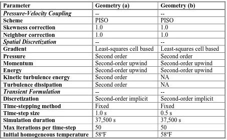
Parameter Geometry (a) Geometry (b)

Method Triangular Triangular

Maximum Element Size 1.05 ft 1.05 ft

Element Size Near Diffusers 0.085 ft 0.085 ft

Element Size along Tank Outer Wall 0.15 ft 0.15 ft

(52)

Figure 2.5: Generated mesh for turbulent regime geometry (left) and laminar regime geometry (right)

2.2.4 Governing Equations

Numerical results are obtained using ANSYS Fluent version 17.1. This CFD package is capable of accurately simulating a plethora of different flow phenomena including, but not limited to laminar and turbulent flow throughout various fluid domains, single and two-phase flows, species transport, and heat transfer effects. As pointed out in the previous subsections in this chapter, Reynolds numbers within stratified chilled-water storage tanks vary

(53)

models are compared with results obtained assuming laminar flow. Both turbulent and laminar simulation results are compared to field data. The flow model and respective geometry that best describes stratified chilled-water storage tank behavior are then used to perform a parametric study to ascertain tank behavior during off-nominal conditions.

Several reasonable simplifying assumptions can be made to facilitate modeling and decrease simulation runtimes. Temperature differences between chilled water in the bottom of the tank and warm water in the top of the tank typically vary between 9oF and 15oF. While these rather insignificant differences in temperature are large enough to induce stratification stemming from density differences, water properties can be assumed to be constant. To capture buoyancy-induced stratification as a result of differences in density, the Boussinesq approximation is employed. The Boussinesq approximation assumes the density throughout the fluid domain is constant, and thus, resulting inertial forces from density differences are negligible, but buoyancy forces in the presence of a non-zero gravitational field are

substantial enough to affect fluid flow [44]. The Boussinesq approximation is given by Equation (2.1):

 

  



TT0



(2.1)

This simplification is valid for:

  (2.2)

With this simplification, the differences in density are linearized about a specified temperature, in which the product of the coefficient of thermal expansion and constant density value is the slope of the linear approximation. As with any linear approximation, it is only valid for small differences in the independent variable, or in this case, water