Two-Locus Sampling Distributions and Their Application
Richard R. Hudson
Department of Ecology and Evolution, University of Chicago, Chicago, Illinois 60637 Manuscript received March 1, 2001
Accepted for publication August 31, 2001
ABSTRACT
Methods of estimating two-locus sample probabilities under a neutral model are extended in several ways. Estimation of sample probabilities is described when the ancestral or derived status of each allele is specified. In addition, probabilities for two-locus diploid samples are provided. A method for using these two-locus probabilities to test whether an observed level of linkage disequilibrium is unusually large or small is described. In addition, properties of a maximum-likelihood estimator of the recombination parameter based on independent linked pairs of sites are obtained. A composite-likelihood estimator, for more than two linked sites, is also examined and found to work as well, or better, than other available ad hocestimators. Linkage disequilibrium in the Xq28 and Xq25 region of humans is analyzed in a sample of Europeans (CEPH). The estimated recombination parameter is about five times smaller than one would expect under an equilibrium neutral model.
L
INKAGE disequilibrium is widely recognized as an multiple linked polymorphic sites. However, at present,these Monte Carlo methods are extremely computation-important aspect of variation in natural
popula-tions (Lewontin1964, 1974;Langleyet al.1974;Lang- ally intensive, and it has been difficult to assess when a
valid estimate of the likelihood is obtained and even
ley 1977). Despite this recognition, there appears to
be no consensus about how to analyze linkage disequilib- more difficult to assess the properties of any statistical
inference based on these methods. rium or even to summarize the levels of observed linkage
In summary, quantifying and interpreting observed disequilibrium when two or more polymorphic sites are
patterns of linkage disequilibrium remain a challenge. observed in a sample of chromosomes. One approach
To address this challenge, we propose in this article has been to calculateD2orr2for all pairs of polymorphic
that one consider polymorphic sites in pairs and utilize sites and plot these values as a function of the distance
likelihood methods appropriate for analyzing a pair of
between each pair of sites. (For examples, seeLangley
polymorphic sites. That is, we suggest that it may be of
1977; Chakravarti et al. 1984; Langley et al. 2000;
use to interpret observed two-site sample configurations
Taillon-Miller et al. 2000.) Since the moments of
in light of the two-site sampling distribution under a these summary statistics are known at least
approxi-simple neutral model, without summarizing the data in
mately under standard neutral models (Ohtaand
Kim-a stKim-atistic such Kim-asD2orr2. When more than two linked
ura1969, 1971;KimuraandOhta1971;Hill1975),
polymorphisms appear in a data set, this approach will this has been useful. However, much information is
entail some loss of information, but a great deal is gained lost in these summary statistics. An alternative analysis
in tractability relative to the full multisite-likelihood
ap-consists of reporting the P value of an exact test of
proach. In this article, we describe some methods of independence for all pairs of sites (e.g.,Macphersonet
calculating (or estimating) two-site sampling
distribu-al.1990;Langleyet al.2000;VieiraandCharlesworth
tions and some applications of these distributions for
2000; however, see Lewontin1995 for an alternative
the analysis of samples from natural populations. to this approach). Unfortunately, this approach gives
Although methods of calculating or estimating two-little sense of whether observed levels of linkage
disequi-locus sample probabilities have been previously de-librium are higher or lower than expected for pairs of
scribed (Golding 1984; Hudson 1985; Ethier and
tightly linked sites.
Griffiths1990), very little use has been made of these Recently, methods for estimating likelihoods under
distributions, in part because of the computational
ef-simple neutral models have been introduced (
Grif-fort that has been necessary to obtain these
probabili-fithsandMarjoram1996;Kuhneret al.2000;Nielsen
ties. However, even inexpensive desktop computers are 2000). In principle these methods should allow the most
now sufficiently fast to calculate these probabilities, at powerful analyses to be carried out on samples with
least for small sample sizes. Furthermore, the required sampling distributions can be made available over the Internet.
Address for correspondence:Department of Ecology and Evolution,
In addition to describing existing methodology, we
1101 E. 57th St., University of Chicago, Chicago, IL 60637.
E-mail: [email protected] extend the methods in several ways. These include
sidering samples in which the ancestral/derived states primary interest, and most results will be for the limiting
case as →0.
of alleles are taken into account. Also, two-locus diploid sample probabilities are calculated. In addition, we de-scribe how these distributions can be used to assess
OBTAINING SAMPLE PROBABILITIES
observed levels of linkage disequilibrium between sites
Recursion equations method: Numerical values of and how they may be used to estimate the
recombina-qu(n;,) can be obtained for small samples by solving a
tion rate parameter of a neutral model.
recursion, originally due toGolding(1984) and further
analyzed byEthierandGriffiths(1990). The reader
should consult these articles for details. For sample sizes
THE MODEL AND NOTATION
⬎40, the linear systems of equations that need to be
We consider a selectively neutral two-locus random solved become quite large. For example, with a sample
union of gametes model with discrete generations and of size 40, the last set of equations that must be solved
Wright-Fisher sampling to produce succeeding genera- has ⬎20,000 equations. However, the system is sparse,
tions (KarlinandMcGregor1968;Ewens1979;Grif- having only nine or fewer nonzero coefficients in each
fiths1981). The population size, assumed constant, is equation. A program to numerically solve Golding’s
re-denoted N. We assume that each locus has the same cursion was written by the author and is available at
neutral mutation rate, although relaxing this assump- http://home.uchicago.edu/ⵑrhudson1. The program
tion is trivial. An infinite-allele model of mutation is utilizes a conjugate gradient method and indexed
stor-assumed, although we focus primarily on the case in ages of the sparse matrices as described byPresset al.
which mutation rates are small, in which case the model (1992) to solve the linear systems.
becomes essentially the same as the infinite-sites muta- Random-genealogies Monte Carlo method:An
alter-tion model. The neutral mutaalter-tion rate at each locus is native to solving Golding’s recursion is to estimate the
denotedu, and the recombination rate between the two two-locus sample probabilities by the method of
Hud-loci is denoted r. For large populations the sampling son(1985). This method is practical for samples of sizes
properties are functions of the composite parameters, up to 100 and perhaps somewhat larger. Briefly, the
4Nu (⬅ ) and 4Nr(⬅ ) (Ohta and Kimura 1969, estimate is obtained by generating a large number of
1971;Hill1975). independent two-locus genealogies (under the neutral
We focus our attention on samples with exactly two model with the appropriate value of) using standard
alleles at each locus. The two alleles at the first locus coalescent machinery (Hudson1983). For each
geneal-are designated A0 and A1; the two alleles at the other ogy, one calculates the probability of the sample
con-locus are designatedB0andB1. (At this point the labeling figuration of interest. The average of these probabilities
is arbitrary, although later, when ancestral and mutant is an estimate ofqu(n;,). Because it is of use later, we
alleles are specified, the labeling will be meaningful.) describe the method in more detail. Before proceeding
A sample ofngametes is randomly drawn from a popula- with this description we note that Monte Carlo Markov
tion at stationarity under the neutral model. The unor- chain methods, such as that of Nielsen (2000), are
dered sample configuration is denoted byn⫽(n00,n01, likely to be very much faster than the method described
n10, n11), where nij is the number of sampled gametes below. Nielsen’s method estimates essentially the same
that carry allele Ai at the A locus and allele Bj at the probability that we consider here but can be used on
B locus. Hence,n00⫹n01⫹n10⫹n11⫽n.The frequen- the much more difficult problem of more than two
cies of theA1allele and theB1allele in the sample are linked sites. However, for estimating the probabilities
p1⫽(n10⫹n11)/nandq1⫽(n01⫹n11)/n, respectively, of all possible configurations for a pair of sites and a
and the frequency in the sample of the A1B1 gamete is given sample size, the method ofHudson(1985) may
p11 ⫽ n11/n. In this notation,D ⫽ p11 ⫺ p1q1 and r2 ⫽ be competitive with the Monte Carlo Markov chain
D2/(p
1(1⫺p1)q1(1⫺q1)) are two commonly employed methods. (For small sample sizes, the point may be
sample measures of linkage disequilibrium. moot, since the sample probabilities have already been
The probability of a particular sample configuration, calculated and tabulated, as described inresults and
n⫽(i,j,k,l), is denotedqu((i,j,k,l);,) or when no applications.For larger sample sizes, the issue remains
ambiguity results asqu(n;,). This sample probability important.) We now describe the method of Hudson
corresponds to the probability given by Ethier and (1985).
Griffiths(1990, Equation 2.14) and the quantity⌽M A two-locus genealogy is produced by generating a ofGolding(1984). We note thatqu((i,j,k,l);,)⫽ random sequence of events, proceeding backward in qu((i,k,j,l); ,), since we assume that the mutation time from the present, as described byHudson(1983).
rate is the same at the two loci. It is qu(n; , ) and The events are coalescent events, in which two lineages
closely related probabilities that are the main foci of merge into a single common ancestor, and
recombina-this article. Because we are interested in polymorphism tion events, in which a single ancestral chromosome
event byEi.The complete ordered sequence of events is Thus to obtain the sample probability, qu(n; , ), we
sum over all branchesjandkand take the expectation
denoted⑀and is referred to as theE-sequence.
Associ-over the joint distribution of⑀and theT-sequence, ated with each event is a specification of which lineage
or lineages are involved. The E-sequence completely
qu(n;,)⫽E
冢
兺
j,kI(⑀,n,j,k)(1⫺e⫺aj)(1⫺e⫺bk)(e⫺(A⫺aj)e⫺(B⫺bk))
冣
determines the topology of the A locus and B locus gene trees. A complete specification of the two-locus
≈E
冢
2兺
j,kI(⑀,n,j,k)ajbk
冣
, (2)genealogy requires that one also specify the time inter-vals between the events. We note, however, that under
the constant population size model, theE-sequence can whereE( ) designates expectation over random
geneal-be generated without regard to the time intervals geneal-be- ogies,jindexes the branches of the A locus tree, andk
tween events. The time interval precedingEiis denoted indexes the branches of the B locus tree. The
approxi-Ti. The ordered sequence of these time intervals is re- mation is for small and is obtained by Taylor
ex-ferred to as theT-sequence. Under the constant popula- panding the exponentials and dropping higher-order
terms in. Since we are interested in small, we consider
tion size model and conditional on theE-sequence, the
the following function: time intervals are independent exponentially
distrib-uted random variables. The mean of Ti depends on
hu(n,)⫽lim
→0
qu(n;,)/2
the configuration of the ancestral lineages during the
interval, which, in turn, depends on the E-sequence.
⫽E
冢
兺
j,k
I(⑀,n,j,k)ajbk
冣
. (3)The calculation of the mean ofTi conditional on the
E-sequence is also described inHudson (1983).
The two-locus genealogy can be summarized as two This function is perhaps best described as the “scaled,
tip-labeled gene trees, one for the A locus and one for small-, likelihood function” and is referred to as the
the B locus. We arbitrarily number the branches of the “scaled likelihood.” The value ofhu(n,) at a particular
A locus tree from 1 to 2n⫺2 and designate the length value ofcan be estimated by generating a large
num-of theith branch byai, measuring time in units of 4N ber,m, of two locus genealogies using the specified value
generations. Note that for any particular branch, say the ofand calculating the sum
ith,aiis the sum of one or more consecutive elements of
theT-sequence. Similarly, the branches of the B locus h
u
典
(n,)⫽ 1
m
兺
m
i⫽1
兺
j,kI(⑀i,n,j,k)aj(i)bk(i), (4) tree are numbered, and their lengths are denoted by
bj.As with the A locus tree, the lengths of the B locus
where⑀iis theE-sequence of theith randomly generated tree are sums of one or more consecutive elements
two-locus genealogy, andaj(i) andbk(i) are the branch
of the T-sequence. It is assumed that the number of
lengths on the same two-locus genealogy. In effect, the
mutations on branchiof the A locus tree, conditional
method simply estimates the expected product of the on its length, is Poisson distributed with mean (/2)ai.
lengths of pairs of branches that, if mutations occurred
The sum of the ai is denoted A and the sum of the
on them, would produce the specified sample configu-lengths of the B locus branches byB. For a given
two-ration. To obtain an estimate of qu(n; , ) we use
locus genealogy, it is a simple matter to check for each
pair of branches, one from the A locus gene tree and 2hu
典
(n,). This is the method of Hudson(1985). In the case of the constant population size model, one from the B locus gene tree, whether a mutation
the method ofHudson(1985) can be made more
effi-on the A locus branch and a mutatieffi-on effi-on the B locus
cient by replacing the randomly generated values of branch would lead to the specified sample
configura-ajbkby their expectation conditional on theE-sequence.
tion, n. This property of the two-locus genealogy
de-That is, we estimatehu(n,) by
pends only on⑀and not on theT-sequence. LetI(⑀,n,
j,k) denote an indicator variable that is one if branch
jon the A locus tree and branchkon the B locus tree
hu
典典
(n,)⫽ 1
m
兺
m
i⫽1
兺
j,kI(⑀i,n,j,k)E(ajbk|⑀i). (5) are such a pair of branches and zero otherwise. IfI(⑀,
n, j, k) equals one, then the sample configuration, n,
This is feasible because aj and bk are sums of one or
would arise if one or more mutations occurred on branch
more consecutive elements of the T-sequence, which
jof the A locus tree, and one or more mutations
oc-are exponentially distributed. Ifajandbkshare no ele-curred on branchkof the B locus tree, and no mutations
ments of theT-sequence in common, then the
expecta-occurred elsewhere on the tree. Thus given⑀ and the
tion of the product is the product of the expectations.
T-sequence, the probability of the configurationnbeing
If they have elements in common, the expectation of
produced by mutations on branchjof the A locus tree
the product is the product of the expectations plus
and branchkof the B locus tree is
the sum of the expectations of the elements that are
common to both. For example, ifajis equal to the sum
of T2 ⫹ T3 andbkisT3 ⫹ T4, then under the constant ing population size can be easily accommodated. A
pro-population size model, the expectation ofajbkis gram to estimateh(n;) using (4) under these models
is available at http://home.uchicago.edu/ⵑrhudson1.
E((T2⫹ T3)(T3⫹ T4))⫽(2⫹ 3)(3 ⫹ 4)⫹ 3, Sequenced samples with two polymorphic sites: In
the previous sections, the samples considered are as-wherei⫽E(Ti|⑀). This follows from properties of the
sayed only at two sites. The intervening and flanking exponential distribution. Thus if hu(n;) is estimated
nucleotide sites may or may not be polymorphic. This
with (5) rather than (4), theT-sequence does not need
is exactly the situation considered byNielsen (2000).
to be generated and a lower variance estimate ofhu(n;
In contrast, we consider now the case where a set of
) is obtained.
contiguous sites are sequenced in each individual and
Ancestral and derived alleles: In the previous
para-all sites are therefore examined, and para-all polymorphisms graphs, we did not specify which alleles were ancestral
in the sequenced segment are detected. Thus, full hap-and which were the mutant (or derived). It is now
com-lotype information is obtained for all sites in the seg-mon to obtain sequence from a closely related species
ment. This is the situation considered byGriffithsand
and infer which alleles are ancestral. The probabilities of
Marjoram(1996) and Kuhneret al. (2000).Nielsen
sample configurations with specified ancestral/derived
states are no more difficult to calculate than the unspeci- (2000),GriffithsandMarjoram(1996), andKuhner
fied configurations. A sample in which the ancestral/ et al. (2000) all analyze the very difficult problem of
derived status of each allele is specified is referred to estimating the probability of samples with arbitrary
as an “a-d-specified” sample, and otherwise the sample numbers of linked sites. In contrast, we now limit
our-is “a-d unspecified.” The algorithm we just described selves to the special case where only two sites are found
can be modified to estimate the probabilities of a-d- to be polymorphic in the sample (and the rest are
mono-specified samples by simply changing the indicator func- morphic), because, in this case, the random-genealogies
tion used. Golding’s recursion can also be modified to method of Hudson (1985) can be easily extended to
calculate a-d-specified sample probabilities. We use the calculate these sample probabilities for a sequenced
convention for a-d-specified samples thatA0andB0de- segment. This can be done as follows.
note the ancestral alleles and A1 and B1 denote the If the segment sequenced isL nucleotides long, we
mutant alleles. For a-d-specified samples, the quantities use anL-locus model, where each locus corresponds to
corresponding to qu(n;,) andhu(n;) are denoted a nucleotide site. We number the nucleotide positions
q(n;,) andh(n;). from 1 (the leftmost site) toL(rightmost site.) Instead
The a-d-unspecified probabilities can be obtained of a two-locus gene genealogy we must consider anL-locus
from the a-d-specified probabilities by summing four gene genealogy. Each site has associated with it a gene
(or fewer) distinct a-d-specified sample probabilities, genealogy or gene tree. The sum of the lengths of the
which result in the same unspecified sample configura- branches of the gene tree of theith site is denoted
i.
tion. That is, we can obtain the a-d-unspecified probabil- We denoteRL
i⫽1i/Lbyseq. We designate the positions
ities with of the two polymorphic sites byxandy.The branches
of the tree of sitexand of the tree siteyare numbered
qu((i,j,k,l);,)⫽[q((i,j,k,l);,)⫹q((k,l,i,j);,)
arbitrarily from 1 to 2n ⫺2, and the length of branch
⫹q((j,i,l,k);,) j of the tree of site x is labeled x,j, and similarly y,k
denotes the length of thekth branch of the tree of site
⫹q((l,k,j,i);,)]/(i,j,k,l),(6)
y. The two-locus sample configuration at sites xand y
where is denoted by n, as before. Hudson (1983) describes
how to generate anL-locus gene genealogy. TheE-series must now include information on where each crossover event occurs along the segment. We focus on the case
(i,j,k,l)⫽
4 ifi⫽ j⫽k⫽ l
2 ifi⫽ jandk⫽landj⬆ k, or if
i⫽ kandj⫽landi⬆j, or if
i⫽ landj⫽kandi⬆j
1 otherwise.
of small mutation rates, and so the infinite-allele model is still appropriate for each site. Letutdenote the total
mutation rate for the set ofLsites andut/Lthe mutation
rate per site. We denote 4Nutbyt. In this notation, if
Inresults and applications, we compare
scaled-likeli-t/Lis small, the expected number of polymorphic sites hood curves for one a-d-unspecified sample and the
isⵑtE(seq), and the probability of no polymorphic sites corresponding a-d-specified configurations. In that
sec-in the sample isⵑE(e⫺tseq). As before, we define ⫽
tion we also address the issue of whether knowledge of
4Nr, but in this case r is the recombination rate per
which alleles are ancestral can improve estimates of.
generation between the leftmost and rightmost sites of
The method of Hudson(1985) can be extended to
the sequenced segment. The probability of the fully any neutral model in which the two-locus genealogy
sequenced a-d-specified sample with two polymorphic can be efficiently generated. In particular, simple island
be represented by a 10-vector, nd ⫽ (n0, n1, . . . , n9). qseq(n,x,y;t,) ⫽ E
冢
兺
j,k
Ix,y(⑀,n,j,k)(1⫺ e⫺tx,j/L)
We use n0 to denote the number of coupling-phase
double heterozygotes (A0B0/A1B1) andn1to denote the ⫻(1⫺ e⫺ty,k/L)
number of repulsion-phase double heterozygotes (A0B1/ A1B0). The numbers of each of the other diploid geno-⫻(e⫺t(seq⫺x,j/L⫺y,k/L))
冣
types are designated byni,i⫽2, . . . , 9. From the vector,
nd, we can count the number of each of the four possible
chromosomes. That is, the vector nd maps
unambigu-≈E
冢
(t/L)2兺
j,k
Ix,y(⑀,n,j,k)xjyke⫺tseq
冣
,ously to the underlying haploid data configuration,
(7) which we denote byn(nd). Under random mating, the
probability ofndisq(n(nd); ,) times the probability where the approximation is obtained by expanding
se-that 2nhaploids of configurationn(nd) when randomly lected exponential terms and dropping terms of order
paired producend. In symbols, (t/L)3 and higher and where I
x,y is an indicator
func-tion, as before, but in this case it depends on the gene qdip(nd;,)⫽b(nd,n(nd))q(n(nd); ,), (10) genealogies of sitexand of site y. Ix,y is one if thejth
where b(nd, n(nd)) is the probability under random
branch of the tree of sitexand thekth branch of the
pairing of getting nd from a haploid configuration
tree of site y are such that mutations on them lead
n(nd). By counting up the possible pairings, one finds to the given a-d-specified sample configurationn. This
that expression for the probability of a sequenced sample is
essentially the same as the expression for the two-locus
b(nd,n)⫽
n!
兿
9i⫽0ni!
n00!n01!n10!n11!
(2n)! 2
n
het, (11)
configuration (2), except for the last term,e⫺tseq. The
analogue ofh(n;) for sequence data, which we denote
hseq(n,x,y;,t), is wherenhetis the number of diploid individuals that are
heterozygous at one or two loci and whereniis theith
hseq(n,x,y;,t)⫽lim
L→∞ qseq
(n,x,y;t,)/(t/L)2, (8)
element ofndandnij,i,j⫽0, 1 are the elements ofn. Now consider the case where the phase of double
wheretis assumed constant (and does not depend on
heterozygotes is not determined by the experimenter.
L). This can be estimated by
In this case, we cannot observe n0 or n1, but we do
observe their sum. We denote the sum byndh.We denote
hseq
典
(n,x,y;,t)⫽ 1
m
兺
m
i⫽1
兺
j,kIx,y(⑀i,n,j,k)xj(i)yk(i)e⫺tseq(i),
the diploid data set in this case bynd⫺9⫽(ndh,n2, . . . ,
n9). Given ndh, the actual number of coupling phase
(9)
double heterozygotes,n0, could be any value from zero
where⑀iis theE-sequence of theith randomly generated to n
dh. Each of these possible values corresponds to a
L locus genealogy, and xj(i) and yk(i) are the branch differentn
dconfiguration. We denote these possiblend
lengths on the trees of site x and site y, respectively. configurations byn
d(i,nd⫺9), wherei⫽0, . . . ,ndh.That
Andseq(i) isseqfor this sameLlocus genealogy. is, ifn
d⫺9 ⫽ (ndh, n2, . . . , n9), then nd(i, nd⫺9) ⫽ (i, In results and applications we compare h(n; ) n
dh⫺ i,n2, . . . ,n9). Then the probability of a diploid
andhseq(n,x,y;,t) to see how much the knowledge configurationn
d⫺9is obtained by summing up the
prob-that there are no other polymorphisms between or near ability of each of these mutually exclusive possiblen
d
the focal pair of sites affects an inference about. The configurations, as:
estimates of hseq(n, x, y; , t) obtained as described
here may be useful for checking other algorithms for q
dip⫺9(nd⫺9;,)⫽
兺
ndh,
i⫽0
qdip(nd(i,nd⫺9);,). (12) estimating sequenced sample configuration
probabili-ties.
Thus, with the haploid sample probabilities in hand, it
Diploid samples:Up to this point, we have considered
is a simple matter to calculate diploid sample probabili-samples consisting of haplotypes. It would be useful to
ties, using (10), (11), and (12). have sample probabilities analogous to q(n; , ) for
Conditional probabilities:Most applications of these
the case of diploid samples. We show here how the two-locus sampling distributions will focus only on pairs
probabilities of diploid samples can be expressed in of sites in which both sites are polymorphic in the
sam-terms of the haploid sample probabilities. ple. This means that rather than q(n; , ), it will be
For diploids, with two alleles segregating at each locus, useful to consider the probability of specific sample
there are 10 distinct diploid genotypes. Often the phase configurations conditional on two alleles segregating in
of double heterozygotes is not determined directly, in the sample at each locus. That is, it is useful to consider
which case there are only 9 distinguishable diploid geno- the conditional probability
types. However, we begin by considering the case where
the haplotypes constituting double heterozygotes are q
(n,,|2 alleles at each locus)⫽ q(n;,)
兺
mq(m;,), (13)
where the summation is over all configurations,m, with The conditional probabilities qc(n;) when plotted
as functions ofare conditional-likelihood curves. Esti-two alleles at each locus. In the limit astends to zero
this becomes mates of three such curves are shown in Figure 2.
Appli-cation of these likelihood curves for estimating are
lim →0
q(n,,|2 alleles at each locus)⫽ h(n;)
兺
mh(m;), (14) described in a subsequent section,Estimating.
Before proceeding to some applications of these sam-ple probabilities we consider briefly the effects of know-which we can estimate without specifying. This
condi-ing which alleles are ancestral and the effects of havcondi-ing tional probability for smallis denotedqc(n;).
full sequence datavs.assessing the variation at only two It may also be of interest to condition on other events.
specified sites. In Figure 3, we show plots ofh(n;) for For example, one may wish to limit consideration to
a set of four a-d-specified samples and hu(n;) for the
polymorphisms in which the rarer allele has frequency
corresponding a-d-unspecified sample. In the plot, we
⬎0.05, or one may wish to condition on precisely the
see that different a-d-specified samples, each corre-marginal allele frequencies observed. These are easily
sponding to the same a-d-unspecified sample, can have calculated by changing the summation in the
denomina-very different likelihood curves. In this case, two of the tor of the right-hand side of (14). Various conditional
configurations have monotonically decreasing likeli-probabilities are utilized in the following sections.
hood curves, and the other two configurations have a
maximum for intermediate values of . However, two
RESULTS AND APPLICATIONS
of the configurations, which have similar curves, have much higher probabilities than the other two
configu-Example sampling distributions:I have used the
Hud-rations. Thus, although knowledge of which alleles are
son(1985) Monte Carlo algorithm (and Equation 4 or
ancestral may in specific instances have an important 5) to estimate h(n;) for all possible two-locus sample
impact on inferences about, on average, knowledge
configurations (with exactly two alleles at each locus)
of which alleles are ancestral may not provide very much for samples sizes of 20, 30, 40, 50, and 100 and a range
more information. This suggestion is supported by the
of values between 0 and 100. These are available at
results concerning asymptotic variances of estimates of
http://home.uchicago.edu/ⵑrhudson1. The program
using many pairs of sites, which is described later. used to estimate these quantities is also available at this
The effects of having full sequence datavs.assessing site. The program actually generates multilocus gene
the variation at only two polymorphic sites are illustrated trees and simultaneously estimates the sample
probabili-in Figure 4, probabili-in which we show plots ofh(n;) andhseq(n,
ties for a range of recombination rates and all possible
x,y;, t) as functions of forn ⫽ (15, 15, 9, 1) and sample configurations simultaneously. The results for
t⫽0.6. In this case, the curves are very similar in shape. sample size 40 have been compared for several
configu-One should be cautious about generalizing from this rations to the results of solving the recursions of
Gold-particular result, but it appears that, for the case where
ing (1984). No significant discrepancies were found.
only two sites are polymorphic, likelihoods based on Thus two very different approaches using entirely
inde-full sequence data may be quite similar to the likelihood pendent computer code produced essentially the same
based on assays of only the pair of sites that are polymor-values for the probabilities of a large number of sample
phic. For other values oftthis may not hold. configurations over a range ofvalues. In addition, the
Assessing observed levels of linkage disequilibrium:
results for large recombination rates converge on the
With the conditional probabilities described above, it free recombination configuration probabilities that are
is possible to assess whether or not the level of linkage easy to calculate with Ewens sampling distribution
disequilibrium observed between a particular pair of
(Ewens 1972) and the assumption of independence
sites is compatible with our neutral model and a speci-of the two sites. These two results give considerable
fied value of . For example, suppose that we have a
reassurance that the Monte Carlo program functions
sample of 90 gametes in which two sites, 1000 bp apart, correctly. The program can also be used to estimate
are assayed and found to be polymorphic, with sample two-locus sample probabilities under the island model
configuration,n⫽ (53, 7, 17, 13). (This is the sample
of spatial structure and under a model with recent
expo-configuration corresponding ton11⫽13 in Figure 1.)
nential growth in population size.
Note that the marginal allele frequencies of the derived Figure 1 shows some conditional sampling
distribu-alleles are 30(⫽ 17⫹ 13) at one locus and 20(⫽ 7⫹
tions for a sample of size 90. This figure shows the
13) at the other locus. We ask the question of whether asymmetric U-shaped distribution of linkage
disequilib-this observed configuration is compatible with the hy-rium, which is typical for low recombination rates, the
pothesis that 4Nrbp (⫽ bp) equals, say, 0.001, whererbp
broad distribution of linkage disequilibrium for values
is the recombination rate per base pair per generation.
ofin the range of 5–20, and the unimodal and nearly
With these assumptions, the relevant recombination pa-normal distribution of linkage disequilibrium for large
rameter for our pair of sites is ⫽ bp 1000⫽ 1.0. To
. An application of these distributions is described in
Figure1.—Conditonal prob-abilities of two-locus sample configurations for samples of size 90. The height of each col-umn gives the probability of the configuration withn11 tak-ing the value on the abscissa, conditional onn11⫹n10⫽30 andn11⫹n01⫽20. Given these marginal frequencies, Dtakes its minimum possible value whenn11⫽0 and its maximum possible value whenn11⫽20. These conditional sample probabilities were calculated with (14) with the denominator equal to the sum over all configurations with the specified marginal allele frequencies. The leftmost column is truncated and should rise to a value of 0.58.
unusually high or low, we examine the distribution ofn 13 have probabilities less than or equal to the observed
configuration. The sum of the probabilities of these conditional on the observed marginal allele frequencies
with ⫽1.0. Conditional on the marginal allele frequen- configurations is approximately 0.028, so our hypothesis
is rejected. That is, we conclude that this sample config-cies, there are only 21 possible sample configurations,
which can be specified by the value ofn11. The condi- uration is quite unusual for ⫽ 1.0 and note that it
would be much more likely if ⫽10. We refer to this
tional probabilities of these configurations for ⫽1.0
are shown in Figure 1 and were obtained using Equation test as the “exact test conditional on the marginals”
(ETCM) and emphasize that it requires that one know 14, with the summation in the denominator of the
right-hand side being over the 21 possible sample configura- or specify.
Suppose now that our pair of polymorphic sites, with tions.
We define a statistical test by summing the conditional n ⫽ (53, 7, 17, 13), had been 100,000 bp apart, in
which case, ⫽ 100. If we examine the conditional
probabilities of all configurations with probabilities less
than or equal to the probability of the observed config- probabilities for this value of (shown on the right in
Figure 1), we find that the sum of the probabilities of uration. If this sum is⬍0.05 we reject our hypothesis.
In our example, the configurations withn11⫽ 8, . . . , configurations with less or equal probabilities isⵑ0.02,
and so the hypothesis would again be rejected. (In this case the configurations with lower probabilities aren11⫽
0, andn11⫽ 14, . . . , 20.) There is too much linkage
disequilibrium in this case. This illustrates that the
Figure2.—The conditional-likelihood curves for three sam-ple configurations. (䊐)n11⫽5. (䊊)n11⫽1. (䉬)n11⫽0. The conditioning in this case is that there are two alleles at each locus in the sample. The three sample configurations aren⫽
(20, 10, 20, 0),n⫽(21, 9, 19, 1), andn⫽(25, 5, 15, 5), which Figure3.—A comparison of the scaled-likelihood functions for an a-d-unspecified sample,hu(n; ), and the four corre-are labeledn11⫽ 0, n11⫽ 1, andn11⫽ 5, respectively. The
marginal allele frequencies are the same for each configura- sponding a-d-specified samples. The top curve, hu(n; ), is equal to the sum of the lower four curves. (䊉)hu ((16, 20, tion. The values ofqc(n;) shown here were estimated with
(14), modified for a-d-specified samples, using scaled likeli- 14, 0);). (䉫)h((16, 20, 14, 0);). (䊏)h((6, 30, 14, 0);). (䉭)h((0, 30, 14, 6);). (䉱)h((0, 20, 14, 16);).
Figure4.—A comparison of (䊏)h(n;) and (䊊)hseq(n,x, y; 2,t) forn⫽(15, 15, 9, 1) andt⫽0.6.hseq(n;x,y; 2,t) was estimated with Equation 9 on the basis of simulations with L⫽10,000 sites andx⫽2500 andy⫽7500. With this choice of xand y, the recombination parameter corresponding to the recombination rate between these two sites is.
Figure 5.—The expected log-likelihood curve, (䊏) E0 (log(qc(n; z))), for0 ⫽5.0 and n⫽ 50. For this curve we
ETCM can reject the null hypothesis due to either too conditioned on the marginal allele frequencies beingⱖ0.1.
(This curve is obtained using (16) and (14) and tabulated
much or too little linkage disequilibrium.
values ofh(n;).) Also shown is a second degree polynomial
This test could be carried out for all possible pairs of
obtained by a least-squares fit to the points on the expected
polymorphic sites in a contiguous region to explore the
log-likelihood curve nearz⫽5.0. (—) Fitted quadratic.
possibility that some sites exhibit unusually high or low levels of linkage disequilibrium. Such sites may be indic-ative of hotspots of recombination or mutation or
epi-pair of sites. The maximum-likelihood estimate of
static selection. This is a complementary approach to
obtained with (15) is denotedˆ. the usual analysis of linkage disequilibrium in which
To characterize the statistical properties of the maxi-Fisher’s exact test of independence is applied to all
mum-likelihood estimate ˆ, it is useful to consider the pairs. It should be noted that, when more than two
expectation of log(qc(n; z)), over the distribution of n
linked sites are considered, there is a statistical
depen-conditional on polymorphism at both sites. That is, we dence between the ETCMs on each pair, and any
inter-consider pretation of the results should bear this in mind.
Estimating:Using independent linked pairs:The condi- E0(log(qc(n;z)))⫽
兺
nqc(n;0)log(qc(n;z)), (16)
tional probabilities qc(n; ) when plotted as functions
ofare likelihood curves. Estimates of three such curves whereE
0indicates expectation given that the true value
are shown in Figure 2. (The estimates are obtained using ofis0. This function can be viewed as a function of
(14) and (4) but for a-d-specified samples.) Most sample bothzand0and can be estimated from our tabulated
configurations lead to monotonically increasing or de- values ofh(n;). An estimate of this function is plotted
creasing likelihood curves, but samples with high but as a function of logzfor0⫽ 5.0 and a sample of size
not complete linkage disequilibrium lead to likelihood 50 in Figure 5. (The conditioning for Figure 5 is that
functions with a maximum at a finite positive value of both sites are polymorphic with the rarer allele having
. Thus the maximum-likelihood estimate of for a frequencyⱖ0.1.) The second derivative of this function
single pair of sites is often zero or infinity. When the
with respect toz, evaluated at the0, is inversely propor-estimate is finite and greater than zero, the confidence
tional to the asymptotic variance of the maximum-interval is clearly large (as indicated by the broad
likeli-hood estimate of . More precisely, if k pairs of sites
hood function). This was noted before by Hudson
are utilized, we expect the variance of the
maximum-(1985) and byHillandWeir(1994). However, if one
likelihood estimator to be approximately
hadkpairs of sites, where each pair is independent of
the other pairs and where each pair of sites has the
Var0,k(ˆ) ≈
1
⫺k(2/z2)E
0(logqc(n;z))|z⫽0 (17) same, then one might be able to obtain a very accurate
estimate of . In this case the overall likelihood, for
forksufficiently large. Here, Var0,kdenotes the variance small, is approximately
of the estimator based onkpairs and with ⫽ 0. With
L(n1, n2, . . . ,nk;)≈
兿
k
i
qc(ni;), (15) the tabulated estimates of h(n; ), one can estimate
the second derivative in (17) and hence the asymptotic
variance of ˆ. However, it may be of most interest to
distributed, then with probabilityⵑ0.95, log(ˆ) will lie in the interval log(0)⫾ 2(0.35), and henceˆ will be within a factor of 2 of the true value. To check this result, I generated 32,000 two-locus samples on the computer, using the conditional sampling probabilities qc(n; ),
conditioning on the appropriate marginal allele fre-quencies. These random two-locus samples were formed
into 1600 groups of 20, andˆ was calculated for each
group. From these outcomes, the estimated variance of log(ˆ) was 0.124, which is very close to the prediction
from the asymptotic analysis (2.5/20 ⫽ 0.125). The
probability of being within a factor of 2 is estimated to be 0.96, also in very good agreement with the asymptotic analysis prediction of 0.95.
In practice, different pairs of polymorphic sites will
Figure6.—Estimates of the asymptotic variance of the loga- be different distances apart and will have different
re-rithm of the maximum-likelihood estimate ofbased on k combination rates. In the case where the physical dis-independent pairs of polymorphic sites. These estimates were
tance between each pair of sites was known and the
obtained with Equation 18, with estimates of the second
deriva-recombination rate per base pair was the same for each
tive of the expected likelihood function. The expected
log-pair of polymorphic sites, then the likelihood fork
poly-likelihood functions were estimated from (16) and tabulated
values ofh(n;). morphic pairs is approximately
L(n1,n2, . . . ,nk;bp)≈
兿
k
i
qc(ni;bpdi), (19) investigate the coefficient of variation of the estimate
of, so we consider instead
wherebpis 4Nrbp,rbpis the recombination rate per base
pair, anddiis the distance in base pairs between theith pair of sites. This likelihood could be used to estimate
bp. The results in the previous paragraph suggest that the lowest variance estimator ofbp will be obtained if sites are separated by a distance such thatbptimes the distance isⵑ5. Ifrbpvaried from one pair of sites to the
In Figure 5, we show, in addition to our estimate of next, but the value ofrbpwere known for each pair of
E0(log(qc(n;z))) for0⫽5.0, a quadratic function ob- sites, say from comparisons of physical and genetic
tained by a least-squares fit to several points nearz⫽5.0. maps, a similar likelihood could be used to estimateN,
Clearly the expected likelihood function is very close the effective population size.
to quadratic for a substantial range ofzin the neighbor- Using the above method, we can estimate the
asymp-hood of 5.0. This suggests that the asymptotic properties totic variance of in a-d-unspecified samples and in
may apply for moderate values ofk.By estimating the diploid samples in which the phase of double
heterozy-second derivative of the expected likelihood functions, gotes is not determined. For the case of a-d-unspecified
we have estimated asymptotic variances (timesk) for a samples of 50 gametes in which ⫽5.0, the asymptotic
set of values of0and plotted the results as a function variance is estimated to be 2.2/k, which is essentially
of0in Figure 6. The plot in Figure 6 shows that pairs the same as what we found for a-d-specified samples.
separated byin the range of 2–15 are best for estimat- Thus, there appears to be little if any gain in knowing
ing. Asdecreases below 2.0, the asymptotic variance which alleles are ancestral when the data consist of
inde-grows rapidly. For larger values ofthe asymptotic vari- pendent linked pairs of sites. A similar asymptotic
analy-ance grows more slowly. sis could be used to determine the optimum sample
To give some feeling for the number of pairs needed size when one can trade off sample size for number of
to get a reasonable estimate ofwe consider a numerical pairs. We do not pursue that analysis here.
example. Suppose that we have data fork⫽20 indepen- Finally we note that, when investigating pairs of
poly-dent pairs of polymorphic sites, where the rare allele morphic sites, the incorporation of gene conversion is
has in every case allele frequency of at least 0.1 and straightforward. It is necessary only to establish an effective
where the recombination rate,0, between the sites of recombination rate as a function of distance that
incorpo-each pair is the same and is in the range from 2 to 10. In rates gene conversion, such asAndolfattoand
Nord-this case, we see from Figure 6 thatk is borg(1998) orLangleyet al.(2000). The
scaled-likeli-ⵑ2.5, and hence the asymptotic standard deviation of hood functions do not need to be recalculated.Frisse
log(ˆ), when estimated from 20 independent pairs, is et al.(2001) recently estimated gene conversion rates
in humans using this method.
Figure7.—Estimates of the medians (ˆ50) of four estima-tors of(each divided by the true value of ). These are based on 10,000 samples of size 50 generated by coalescent-based Monte Carlo simula-tions. The four estimators are described in the text.
Using many linked sites:In the previous sections, we recombination rate between the ends of the segment
observed andbeing the mutation parameter associated
considered one or more linked pairs of sites, where
each pair is independent of the others. We now consider with the entire segment. Figures 7 and 8 show estimates
of the medians and the 10th and 90th percentiles of the case where more than two linked polymorphic sites
are assayed in a single sample. In this situation, full the distribution ofˆCLfor a range ofvalues. The same
quantities were estimated for three other estimators that likelihood considering all polymorphisms
simultane-ously is the proper approach.GriffithsandMarjoram have been described in the literature. These estimators
are␥(HeyandWakeley1997),Cwak(Wakeley1997),
(1996),Kuhneret al.(2000), andNielsen(2000) have
provided Monte Carlo methods for estimating these andCHRM (Wall2000). Each estimator was calculated
for each of 10,000 samples (each of size 50
chromo-likelihoods. However, at present the methods of
Grif-fithsandMarjoram(1996) andKuhneret al.(2000) somes). [These results for␥(HeyandWakeley1997),
Cwak(Wakeley1997), andCHRMwere kindly provided by
are difficult to employ due to the very large
computa-tional requirements and the difficulty in determining Jeff Wall.]
The figures show that the estimator, Cwak, performs
when adequate convergence has been obtained. The
approach ofNielsen(2000) is less computationally de- poorly compared to the other estimators shown. The
estimator Cwak is an improved version of the estimator
manding and goes some way toward solving this
prob-lem. However, the properties of full-likelihood estima- ofHudson(1987), which would perform slightly more
poorly thanCwak.
tors have not been explored, and the computation
requirements for this exploration are daunting. As an The estimator␥has a considerably lower 90th
percen-tile than the other estimators. This is desirable as long alternative we consider a composite (or pseudo-)
likeli-hood obtained by using (19), where the summation on as the 90th percentile is larger than the true value.
Unfortunately, for largeand ⫽ /4, the 90th percen-the right-hand side is over all pairs of sites. This is an
approach suggested byHudson(1993). Because of the tile of␥falls below the true value. In addition, it has a
median considerably below the true value and a 10th statistical dependence between different pairs of sites,
this expression is not the true likelihood. We can never- percentile well below the 10th percentile of ˆCL and
CHRM. Thus, for these parameter values␥ has a strong
theless maximize this function to obtain an estimate
of bp, which is denotedˆCL, where the subscript “CL” tendency to underestimate. For other parameter
val-ues HeyandWakeley(1997) showed that ␥has little indicates an estimate based on composite likelihood.
Once the two-locus sampling-scaled likelihoods (h(n; bias or a bias in the opposite direction.
The medians of the estimatorsˆCLandCHRMare close
)) are tabulated, calculating these composite
likeli-hoods is very fast, and hence the statistical properties to the true , for ⬎ ⵑ4.0 for the case of ⫽ and
for ⬎ 10 when ⫽ /4. The 10th percentiles ofˆCL
of this estimator can be explored.
To assess the quality of this composite-likelihood esti- andCHRMare considerably closer to the true value than
the 10th percentiles of the other estimators. Their 90th mator,ˆCLwas calculated for a large number of samples
generated by coalescent methods. The samples were percentiles are much closer to the true value than the
90th percentile ofCwakbut as mentioned above are not
generated by the method ofHudson(1983), according
estima-Figure8.—Estimates of the 90th (ˆ90) and 10th (ˆ10) per-centiles of the distributions of four estimators (divided by the true value of). These were es-timated with the same samples used in Figure 7.
torsˆCLandCHRMappear to be quite similar. Overall, it the values reported here for are, in fact, estimates
of 4Nr, where ris the female recombination rate. The
appears that the estimatorspandCHRMare substantially
superior to the other two estimators (at least for the estimates were 9⫻10⫺5, 8.8⫻10⫺5, and 9 ⫻10⫺5for
all 39 sites, for the 14 sites of Xq25, and the Xq28 sites, parameter values investigated). The estimator ˆCL has
considerable flexibility that may make it of broader use. respectively. These results suggest that there is no overall difference in recombination rates in the Xq25 region Since it does not rely on surveying or sequencing of all
sites, it can be applied to data collected on previously compared to the Xq28 region. The effective population
size of humans has been estimated from levels of DNA identified single nucleotide polymorphisms (SNPs) or
in surveys of regions with intervening gaps. Also, as polymorphism to beⵑ104and the recombination rate
per base pair, though quite variable, is for this region indicated earlier, incorporating gene conversion is
straightforward and does not require reestimating any on average ⵑ10⫺8. Thus we might expect thatbp≈4⫻
10⫺4 or about five times larger than we estimate from
of theh(n;) values.
Finally, since ˆCL is so quick to calculate (once the the X chromosome data.
The linkage disequilibrium at each of the 741 (⫽39⫻ scaled likelihoods are in hand), one can afford to carry
out simulations to characterize the properties of an esti- 38/2) possible pairs of sites was evaluated by the ETCM,
described inAssessing observed levels of linkage
disequilib-mate. For example, if the sampling procedure employed
to collect the data is well specified and simple, then rium, assumingbp⫽ 9⫻ 10⫺5. A total of only 7 pairs,
orⵑ0.9% of the pairs, showed unusual two-locus
con-computer-generated samples can be used to study the
distribution of the logarithm of the ratio of the compos- figurations (with P ⬍ 0.025) using the ETCM. This is
somewhat fewer than one would expect by chance when ite likelihood of the data atˆCLto the likelihood at the
true value of for a range of values and in this way carrying out this many tests. Thus, overall, our analysis
does not support the presence of a low recombination obtain confidence intervals.
An application to human polymorphism data: We rate region in Xq25, as suggested by Taillon-Milleret al.However, it should be noted that 6 of the 7 significant
close by estimatingfrom a survey of human variation
on the X chromosome (Taillon-Miller et al. 2000). pairs involve sites from the Xq25 region, and the seventh
is immediately adjacent to the Xq25 region. Of the 6 In this study, 39 SNPs were surveyed in three population
samples. In the following, only the sample of 92 CEPH significant pairs in the Xq25 region, 5 show unusually
large linkage disequilibrium, but the 6th shows
unusu-males is considered. The parameter bp was estimated
by maximizing the composite likelihood for (i) all 39 ally low linkage disequilibrium. The latter pair of sites
is separated by 30 kb andD⬘for the pair is 0.22. The five SNPs, (ii) the 14 SNPs in Xq25, and (iii) the 10 SNPs
in or near Xq28. For loci on the X chromosome, using pairs showing significantly large linkage disequilibrium
from the Xq25 region were among the pairs identified theh(n;) functions described for autosomal loci will
result in an estimate of 2Nr, whereris the per-generation by Taillon-Miller et al. as showing significant linkage disequilibrium by a Fisher’s exact test. In Figure 9, the recombination rate in females andNis the total effective
population size. In the following, the estimates returned values of r2 are plotted for all pairs of sites within the
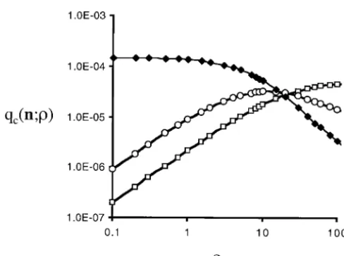
Figure9.—A plot ofr2vs.distance for poly-morphic sites on the X chromosome in a CEPH sample of Europeans. The sites in the Xq25 region are indicated by open circles and those from the Xq28 region by solid squares. The points withx’s over them (all from Xq25) have significantly unusual linkage disequilibrium by the ETCM test. The curve is the expected value ofr2in samples of this size conditional on all alleles having frequency⬎0.32. See text.
pairs within the Xq28 region (10 sites or 45 pairs). LITERATURE CITED
Taillon-Milleret al.also displayed this plot. In the figure Andolfatto, P.,andM. Nordborg,1998 The effect of gene conver-those sites that showed significantly large or small link- sion on intralocus associations. Genetics148:1397–1399.
Chakravarti, A., K. H. Buetow, S. E. Antonarakis, P. G. Waber,
age disequilibrium givenbp⫽9⫻10⫺5, using the ETCM
C. D. Boehmet al., 1984 Nonuniform recombination within
test, are shown withx’s. Also shown in Figure 9 is the the human beta-globin gene cluster. Am. J. Hum. Genet.36:
expected value ofr2 conditional on the frequencies of 1239–1258.
Ethier, S. N.,andR. C. Griffiths,1990 On the two-locus sampling
the minor alleles being ⬎0.32. These were calculated
distribution. J. Math. Biol.29:131–159.
with the tabulated h(n; ) values for a sample of size Ewens, W. J.,1972 The sampling theory of selectively neutral alleles.
92. The fit to the data appears to be fairly good, but Theor. Popul. Biol.3:87–112.
Ewens, W. J.,1979 Mathematical Population Genetics.Springer-Verlag,
there does appear to be some tendency for Xq28 pairs
Berlin.
to fall below the line for larger distances and to be above Frisse, L., R. R. Hudson, A. Bartoszewicz, J. D. Wall, J. Donfack the line for shorter distances. In contrast, the Xq25 sites et al., 2001 Gene conversion and different population histories may explain the contrast between polymorphism and linkage
appear to scatter on both sides of the curve.
disequilibrium levels. Am. J. Hum. Genet.69:831–843.
Golding, G. B.,1984 The sampling distribution of linkage disequi-librium. Genetics108:257–274.
CONCLUSIONS Griffiths, R. C.,1981 Neutral two-locus multiple allele models with
recombination. Theor. Popul. Biol.19:169–186.
Two-locus sample probabilities offer a useful tool for Griffiths, R. C.,andP. Marjoram,1996 Ancestral inference from
samples of dna sequences with recombination. J. Comput. Biol.
analyzing linkage disequilibrium levels from population
3:479–502.
surveys. Carrying out tests of significance for pairs of
Hey, J.,andJ. Wakeley,1997 A coalescent estimator of the
popula-sites and estimatingfrom many sites is computationally tion recombination rate. Genetics145:833–846.
Hill, W. G.,1975 Linkage disequilibrium among multiple neutral
quick, once the two-locus sample probabilities are in
alleles produced by mutation in a finite population. Theor. Popul.
hand. A composite-likelihood approach for estimating
Biol.8:117–126.
with more than two linked sites appears to work as Hill, W. G.,andB. S. Weir,1994 Maximum-likelihood estimation
well as the method of Wall (2000) and better than of gene location by linkage disequilibrium. Am. J. Hum. Genet.
54:705–714.
otherad hocmethods. Of course, none of thesead hoc
Hudson, R. R.,1983 Properties of a neutral allele model with
intra-methods should be used when full-likelihood intra-methods genic recombination. Theor. Popul. Biol.23:183–201.
are computationally feasible. Hudson, R. R.,1985 The sampling distribution of linkage
disequilib-rium under an infinite allele model without selection. Genetics The author is grateful to Jeff Wall and Tony Long for useful discus- 109:611–631.
sion. Also, I am indebted to Jeff Wall for providing most of the numbers Hudson, R. R.,1987 Estimating the recombination parameter of a going into Figures 7 and 8 and to P. Taillon-Miller for providing finite population mode. Genet. Res.50:245–250.
Karlin, S.,andJ. McGregor,1968 Rates and probabilities of fixa- Macpherson, J. N., B. S. WeirandB. Leigh,1990 Extensive linkage disequilibrium in the achaete-scute complex ofDrosophila
melano-tion for two locus random mating finite populamelano-tions without
selection. Genetics58:141–159. gaster. Genetics126:121–129.
Nielsen, R.,2000 Estimation of population parameters and
recom-Kimura, M.,andT. Ohta,1971 Theoretical Aspects of Population
Genet-ics.Princeton University Press, Princeton, NJ. bination rates from single nucleotide polymorphisms. Genetics 154:931–942.
Kuhner, M. K., J. YamatoandJ. Felsenstein,2000 Maximum
likeli-hood estimation of recombination rates from population data. Ohta, T., andM. Kimura, 1969 Linkage disequilibrium due to random genetic drift. Genet. Res.13:47–55.
Genetics156:1393–1401.
Langley, C. H.,1977 Nonrandom associations between allozymes Ohta, T.,andM. Kimura,1971 Linkage disequilibrium between two segregating nucleotide sites under the steady flux of mutations in in natural populations ofDrosophila melanogaster, pp. 265–273 in
Lecture Notes in Biomathematics,Vol. 19, Measuring Selection in Natural a finite population. Genetics68:571–580.
Press, W. H., S. A. Teukolsky, W. T. VetterlingandB. P. Flannery,
Populations, edited byF. B. ChristiansenandT. M. Fenchel.
Springer-Verlag, New York. 1992 Numerical Recipes in C.Cambridge University Press, Cam-bridge, UK.
Langley, C. H., Y. N. TobariandK. Kojima,1974 Linkage
disequi-librium in natural populations ofDrosophila melanogaster.Genetics Taillon-Miller, P., I. Bauer-Sardina, N. L. Saccone, J. Putzel,
78:921–936. T. Laitinen et al., 2000 Juxtaposed regions of extensive and
Langley, C. H., B. P. Lazzaro, W. Phillips, E. Heikkinen and minimal linkage disequilibrium in human xq25 and xq28. Nat.
J. M. Braverman, 2000 Linkage disequilibrium and the site Genet.25:324–328.
frequency spectra in thesu(s)andsu(wa)regions of theDrosophila Vieira, J.,andB. Charlesworth,2000 Evidence for selection at
melanogaster Xchromosome. Genetics156:1837–1852. the fused locus ofDrosophila virilis. Genetics155:1701–1709.
Lewontin, R. C.,1964 The interaction of selection and linkage. I. Wakeley, J.,1997 Using the variance of pairwise differences to esti-General considerations; heterotic models. Genetics49:49–67. mate the recombination rate. Genet. Res.69:45–48.
Lewontin, R. C.,1974 The Genetic Basis of Evolutionary Change.Co- Wall, J. D.,2000 A comparison of estimators of the population lumbia University Press, New York. recombination rate. Mol. Biol. Evol.17:156–163.
Lewontin, R. C.,1995 The detection of linkage disequilibrium in