On a finite buffer problem

(1)

ON A FINITE BUFFER PROBLEM

Bih-Hwang Lee

and

Arne A. Nilsson

Center for Communications and Signal Processing

Department of Electrical and Computer Engineering

North Carolina State University

December 1988

(2)

1. INTRODUCTION

In data communication, there are three major components, the source

system, the transmission medium, and the destination system. Generally,

the source system contains an input device and a transmitter and the

destination system contains an output device and a receiver ( Figure 1 ). In

this paper, we will focus only on the source system.

INPUT

DEVICE

TRANSMISSION TRANSMITTER

MEDIUM RECEIVER

OUTPUT

DEVICE

) \..~----..._y, - - - - '

DESTINAnON SYSTEM

,"""---...

. , - - - ' )

Y

SOURCE SYSTEM

Figure 1 communication model

The input device can be any data generator or data handling machine. If

the input device is an image coder, the image Intorrnatlon is manipulated

into a series of digital data by the coder, and then the transmitter sends

the data to the transmission medium upon receiving the data from the

coder. The data can immediately be transmitted by the transmitter if the

transmission rate of the transmitter is greater than the rate of the coder.

Unforturnately, the transmission rate of a transmitter is sometimes less

(3)

I

~GE

CODER

I

1

BUFFER

I 1

lRANSWTIER

I

TRANSMISSION

MEDIUM

Figure 2 a buffer in the source system

In order to prevent the data loss, we need a buffer in which the excess

input to the transmitter is temporarily stored ( Figure 2 ). An interesting

question is that of how large a buffer we need. Of course, there will be no

loss if we have an infinite buffer, but this is very inefficient and also

totally unrealistic. We also know that if the size of the buffer is small,

the loss can be considerable, unless we adapt a smaller rate of a coder;

however, this implies a degraded performance. Consequently, we have to

face a trade-off problem, which is to decide the optimum buffer size to

achieve the required performance.

In this paper, we assume that the transmission rate of the coder is

much greater than that of the transmitter, so the transmitter receives the

entire input data instantaneously. Thus, the data has to be stored in a

buffer before being transmitted, otherwise, the loss of data is inevitable.

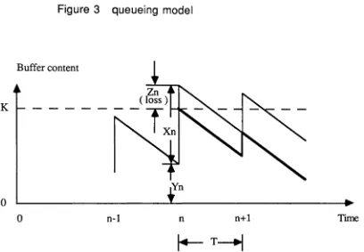
2. ANALYSIS

For a finite-capacity resource system, a queueing model is usually a

good tool to describe the system ( Figure 3). We assume that (1) this is a

FCFS system, (2) the inter-arrrival time between each input is a constant

time period, T, and (3) the amount of data entering the buffer at each input

time is a generally distributed random variable whose probability

distribution function is denoted by B(x). According to this, the queueing

system can be said to be a D/G/1 with variations, ie., a D/G/1 queue with

(4)

PERIODIC INPUT

1

FINITE QUEUEI

Figure 3 queueing model

Buffer content

K

Yn

o

n-l n n+l Time

Figure 4 an embedded Markov chain description

The system can be analyzed by an embedded Markov chain ( Figure 4 ).

Let Ynand X_n represent the buffer content, in bits, at time n and the

message, in bits, entering the buffer at time n respectively. Any excess of

the buffer's capacity, which is K bits, is lost. The amount of loss at time n

is denoted by Zn ' where n = 0,1,2, . .. · For simplicity, let us assume that

the transmission rate of the transmitter is one bit per second, we find

Y n+1

= [

min ( Yn+ Xn ' K ) - T

r

z

_n = [Y_n + X - K_n ]+ · where [ x

I'

= max [ 0, x ] ·

(1)

(5)

Let Wn+1 (y) represent the probability distribution function of Yn+1· Then,

using some probability properties, we get Wn+1 (y) as follows.

Wn+1 (y) = Pr { Yn+ 1

s

y}

= Pr { [ min ( Yn + X_{n '} K ) - T

t

s

y}

= Pr { min (

Y

_{n + Xn ' K ) - T}

s

y}

= Pr {

Y

_{n + Xn}

s

y+T < K or K-T

s

Y }

= Pr {

Y

n + Xn

s

Y+T < K } + Pr { K-T $; Y }

= Pr {

Y

_{n + Xn}

s

y+T and y+T < K } + Pr { K-T

s

Y }

= Pr { Yn + Xn$;y+T } * Pr { y+T < K } + Pr { K-T

s

Y }

= Pr {

Y

n

s

y+T-x

I

Xn=x } * Pr { y < K-T } + Pr { K-T

s

Y }

== {

f:+

T Wn ( Y+T-x ) d B (

x ) }

* Pr { y< K-T } + Pr { K-T

s

Y }

y+T

fa

Wn ( Y+T-x ) d B ( x )

1

o

s

y

< K-T

y~ K-T (3)

(5)

Let us represent the stationary distribution for Yn+1

by

w (

y )

=

lim Wn+1( Y ) (4)

n~oo

where we assume that the limit exists. W(y) will be the stationary

distribution for the buffer content, and also this limiting distribution is

independent of the initial state

Yo.

Thus we have y+T

fo

W ( Y+T-x ) d B ( x ) 0

s

Y< K-T

W(y)

={

(6)

loss at time n. Using some probability properties, we have

Ln

=

Pr {

Zn

s

Z }

= Pr { [ Yn + X_{n -} K

I'

s

z }

=

Pr { Yn + X_{n -} K ~ z }

=

fo

oo

Pr { Yn

s

z + K - x

I

x,

=

x} d B ( x )

=

fo

oo

W

n (

z-K-x )

d B (

x)

z+K

=

fo

Wn ( z+K-x) d B ( x ) ·

Similarly, let us represent the stationary distribution for Zn by

L ( Z )

=

lim i., (z )

n~oo

(6)

(7)

and the limit must exist. L(z) will be the stationary distribution for the

amount of loss, and this limiting distribution is independent of the initial

state

Zoe

Thus we have

z-K

L ( z )

=

fo

W ( z+K-x) d B ( x ) · (8)

Until now, we have obtained W(y) and L(z) for the system. In the next

section, we will select a specific probability distribution function for

(7)

3. SOLUTION FOR THE ERLANG DISTRIBUTED DATA INPUT

In many applications, like telephone traffic theory and data

manipulation, the Erlang distributed random service time has been widely

used. For such a service demand, we have obtained the solution to the

integral equation of the probability distribution function of the buffer

content. If the probability distribution function B ( x) and the probability

density function b ( x) are given as :

k-1 i

B ( x )

=

1 _

e-k~x

" " (kJlx)

.L..J

·

_{I .}I i=0

d ku (

kux

)k-1

b ( x )= - B ( x ) = r- e-k~x ,

dx ( k-1 ) I

(9)

(10)

then, based on the structure of the probability density function, we guess

a solution of the form to be :

k

W(y) =

L

aj

e-~iY

i=0

where ~o

=

0 . (11)

Using the integral equation, we derive it as follows.

y+T

W ( y) =

fa

W ( Y+T-x) d B ( x )

v-r

k k-1

=

1 L

a·

e-~'

(Y+T-x) kJl ( kJlX )

e-k~x

dx

a i=0 I ( k-1 ) !

k

=

L

aj

e-~I(y+T)

(kJl)k 1 I fY+TXk-1

e-(k~-~i)X

dx

1=0 (k-1). 0

k k k k k-n

=

L

<Ij

e-~Ye-~IT

(kJl) -

L

<lj

e-~I(y+T) (kJl)ke-(1CJ1-~,)(Y+T)

L

(y+n

(8)

k

=

L

(Xi

e-

lliY

i=Q

(12)

Fortunately, the solution is obvious if the following two equations hold.

and

(13)

n

=

1,2, ... ,k (14)

Let us first consider the transcendental equation, which is

This is a kth-root equation and ~i can be found as below.

ku (R.T _i21ti )11k (~.T+j21ti)/k

-~ = etJ1 _e ₌e 1

kJl-~i

where j = -v-1 ·

i = 1, 2, ... ,k

i= 1,2, ... ,k

(15)

(16)

In order to obtain ( x . , We need to solve k+1 linear equations of the form

(9)

(17)

n= 1,2, ... ,k k

I

(Xi =0

i= 0 (kJl-~i)D

and make sure that the boundary condition W ( K-T ) = 1 is satisfied.

Thus, the probability distribution function of the buffer content, W(y), has

been obtained.

Now, the probability distribution function of loss L ( z ) can easily be

found by solving the integral equation below.

z+K

L ( z )=

fo

W ( z+K-x) d B ( x )

z-F z+K

=

1

d B ( x)

+

J

W ( z+K-x) d B ( x )

o

z+T

k k ~n

=

B ( z+T ) +~ (x. e-kl!(Z+

n

~ [k/J.(Z+T)] e~i [(n/k+1)T-Kl+j21tni/k (18)

~ I

£.J

(k-n)!

1=0 n=1

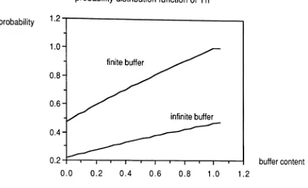
4. EXAMPLE

For specified parameters, the probability distribution function of

buffer content, W(y), and of loss, L(z), have been found. For the parameters

of k=2, Jl= 1.1, and K=2 ( bits ), the curve of the probability distribution

function of buffer content, W(y) , is shown in Figure 5 and the probability

of no loss is 94% in this case. Furthermore, we know that if the buffer

size is increased, the loss is decreased. If the buffer size is increased

immensely, i.e., an infinite buffer system, the probability distribution

function of buffer content has also been found, and of course, there is no

loss. The curve of the probability distribution function of buffer content in

(10)

probability distribution function of Yn

probability

1.2.,---

--..

buffer content

1.2 1.0

0.8 0.6

0.4 0.2

finite buffer

0.2;-...,..-r--..--...-,r----r--~__r-~....,.._--....___1

0.0 0.4 0.8

0.6 1.0

Figure 5 probability distribution functions for finite and infinite buffer

5. CONCLUSION

The buffer problem is an important factor in a queueing system. In

other words, if the capacity of a system is finite, the loss has to be

considered. Although a small buffer can minimize cost and a smaller

transmission rate of a coder can reduce the loss of data, these

characteristics will degenerate the performance of a system. A goOd

performance can be obtained by using a bigger buffer, but the cost may be

prohibitive. However, we can use the model derived in this paper to

(11)

6. REFERENCES

[1] L. Kleinrock, Queueing system Vol. 1 : theory, Wiley, 1976.

[2] D.

J.

Daley, "Single-server Queueing System with Uniformly Limited

Queueing Time", J. Austral. Math. Society 4 ( 1964) pp. 489-505.

[3] J. W. Cohen, The Single server Queue, North Holland publishing Co.,

Amsterdam, 1969.

[4] W. Stallings, Data and Computer Communications, Macmillan