Non-Classical Damping Properties and Modal Correlation Coefficient for Dynamic Analysis of Structures

ABSTRACT

BOSE, MRINAL KANTI. Non-Classical Damping Properties and Modal Correlation Coefficient for Dynamic Analysis of Structures. (Under the direction of Abhinav Gupta and Ajaya Gupta.)

The seismic response of secondary systems depends, in addition to their uncoupled dynamic characteristics, on the interaction with primary structures supporting them. This dissertation presents a verification study of the formulations to evaluate the seismic response of non-classically damped building-piping systems by modal synthesis approach. The existing studies consider only simple representative primary-secondary systems. No real-life like coupled system such as building-piping was used in these studies. Further, the majority of simple systems considered in these studies do not represent realistic coupled systems with significant effect of non-classical damping as they have either high values of mass ratios or systems with detuned modes.

In this dissertation, different configurations of simple representative systems as well as real-life like building-piping systems are considered. Responses obtained from modal superposition time history analyses as well as response spectrum analyses are compared with the corresponding responses obtained by Brookhaven National Laboratory from the direct integration time history analyses. Modal superposition time history analyses results and direct integration time history analyses results are almost identical. The mean and standard deviation of responses from response spectrum analyses are close to the corresponding values evaluated using direct integration time history analysis. In addition to the verification results, a detailed discussion is also presented on the significance of non-classical damping. It is shown that the effect of non-classical damping is significant in systems that have nearly tuned modes and sufficiently small values of modal mass ratios. It is also illustrated that composite modal damping is an alternate form of classical damping that can result in incorrect responses in non-classically damped systems. Possible reasons for numerical and modeling differences that can occur in real-life like building-piping system are identified and their effect on the dynamic characteristics of the coupled system is illustrated.

NON-CLASSICAL DAMPING PROPERTIES AND MODAL

CORRELATION COEFFICIENT FOR DYNAMIC ANALYSIS OF

STRUCTURES

by

MRINAL KANTI BOSE

A dissertation submitted to the Graduate Faculty of North Carolina State University

in partial fulfillment of the requirements for the Degree of Doctor of Philosophy

CIVIL ENGINEERING

Raleigh 2001

APPROVED BY:

BIOGRAPHY

Mrinal Kanti Bose received his Bachelor of Civil Engineering degree from Jadavpur

University, Calcutta, India, in 1990. He received his Master of Civil Engineering from

the same university in 1992. Then he worked in Bhabha Atomic Research Center, India

and his field of research was structural mechanics. He came to North Carolina State

University in 1996 for Ph.D. in Structural Engineering. During his study, he worked as

Research Assistant in the Center for Nuclear Power Plant Structures, Equipment and

Piping, at North Carolina State University.

His research interest includes structural dynamics, finite element analysis and

ACKNOWLEDGEMENTS

This research was partially supported by the Center for Nuclear Power Plant

Structures, Equipment and Piping at North Carolina State University. Resources for the

Center come from the dues paid by member organizations and from the Civil Engineering

Department and College of Engineering in the University.

The author wishes to express his appreciation to Dr. Abhinav Gupta and Dr.

Ajaya Gupta for their guidance throughout the course of this research. Appreciation is

TABLE OF CONTENTS

Page

LIST OF TABLES ……….. vi

LIST OF FIGURES ……….…... vii

PART I INTRODUCTION ……….. 1

Introduction ………. 2

Objective ………..……… 8

Organization ……….…….. 9

References ………. 11

PART II VERIFICATION OF METHODS FOR EVALUATING SEISMIC RESPONSE OF NON-CLASSICALLY DAMPED PRIMARY-SECONDARY SYSTEMS: SIMPLE COUPLED SYSTEMS ………… 13

Abstract ……… 14

Introduction ……….. 15

Coupled Equation of Motion ……… 18

Eigenvalue Problem ………. 20

Coupled System Response ……… 23

Time History Analysis ………. 24

Response Spectrum Analysis ……… 24

Damping Matrix of The Coupled System ……… 26

Description of Benchmark Problems: Simple Systems ………... 28

Validation Results: Simple Systems ……… 29

Significance of Non-Classical Damping ……….. 32

Conclusions ……….. 39

Acknowledgements ……….. 41

References ……….…... 42

PART III VERIFICATION OF METHODS FOR EVALUATING SEISMIC RESPONSE OF NON-CLASSICALLY DAMPED PRIMARY-SECONDARY SYSTEMS: BUILDING-PIPING SYSTEMS ……….… 51

Abstract ……… 52

Introduction ……….. 53

Coupled Problem ………... 55

Secondary System Residual Vectors ………... 56

Description of Building-Piping Systems ……….…..…. 60

Validation Results: Building-Piping Systems ……… 62

Conclusions ……… 66

Acknowledgements ………..……….. 68

References ………..… 69

PART IV A NEW METHOD TO EVALUATE CORRELATION COEFFICIENT FOR COMBINING MODAL RESPONSES ……… 84

Abstract ………... 85

Introduction ………. 86

Modal Superposition ……….. 87

Modal Correlation Coefficient ……….…….. 89

Limitations of the Existing Formulations ………... 92

Proposed Formulation ………. 94

Conclusions ……… 97

Acknowledgements ……… 99

References ………. 100

PART V SUMMARY AND CONCLUSIONS ……… 128

Summary and Conclusions ……… 129

Contributions to Industry Practice ……… 132

Recommendation for Future Work ……….. 132

References ……… 134

APPENDIX A.1 ……… 135

APPENDIX A.2 ……… 153

APPENDIX B.1 ……….. 171

APPENDIX B.2 ……… 187

LIST OF TABLES

Page

PART II VERIFICATION OF METHODS FOR EVALUATING SEISMIC

RESPONSE OF NON-CLASSICALLY DAMPED PRIMARY-SECONDARY SYSTEMS: SIMPLE COUPLED SYSTEMS

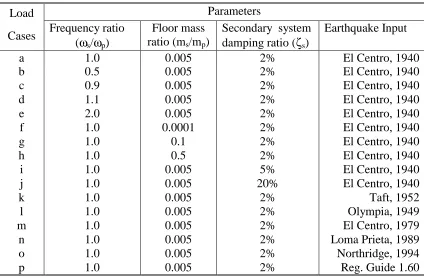
1. Values of Parameters for Various Load Cases of a Particular

Primary-Secondary Configuration ……… 44

PART III VERIFICATION OF METHODS FOR EVALUATING SEISMIC RESPONSE OF NON-CLASSICALLY DAMPED PRIMARY-SECONDARY SYSTEMS: SIMPLE COUPLED SYSTEMS 1. Frequencies and Damping Ratios for Uncoupled Systems ……… 70

2. Spring Forces (kN) in Secondary System ………. 70

3. Uncoupled Primary System Frequencies ……… 70

4a. Uncoupled Secondary System Frequencies, Case 1 ……….… 71

4b. Uncoupled Secondary System Frequencies, Case 2 ………...… 72

5. Coupled System Frequencies, Case 1 ………. 73

PART IV MODAL CORRELATION COEFFICIENT: A NEW PERSPECTIVE 1. Values of key frequencies f₁d and f_r for twelve earthquake records (Gupta et al. 1996) ……….……… 102

LIST OF FIGURES

Page

PART II VERIFICATION OF METHODS FOR EVALUATING SEISMIC

RESPONSE OF NON-CLASSICALLY DAMPED PRIMARY-SECONDARY SYSTEMS: SIMPLE COUPLED SYSTEMS

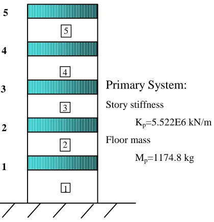
1. Primary System of Benchmark Problem 1,2 and 3 ………..….. 45

2. Secondary System of Benchmark Problem 1 ……….……. 45

3. Secondary System of Benchmark Problem 2 ………. 45

4. Secondary System of Benchmark Problem 3 ……… 45

5. Ratio of element forces from Response Spectrum and Time History analyses, Benchmark Problem 1 ……….. 46

6. Ratio of element forces from Response Spectrum and Time History analyses, Benchmark Problem 2 ………. 46

7. Ratio of element forces from Response Spectrum and Time History analyses, Benchmark Problem 3 ……….. 47

8. Variation of modal and total force in element number 8, Benchmark Problem 1 (Case m) ……… 47

9. SDOF Primary-SDOF Secondary, (2-DOF Coupled System) ………… 48

10. Force in element number 8, Benchmark Problem 1. (El Centro 1940 input) ……… 48

11. Leading diagonal term C11 of Classical Damping Matrix Ccl, 2-DOF coupled system ………..………. 49

12. Off diagonal term C12 of Classical Damping Matrix Ccl, 2-DOF coupled system…………..……….. 49

13. Trailing diagonal term C22 of Classical Damping Matrix Ccl, 2-DOF coupled system ………...……… 50

14. Element force in secondary oscillator, 2-DOF coupled system (El Centro 1940 input) ……… 50

PART III VERIFICATION OF METHODS FOR EVALUATING SEISMIC RESPONSE OF NON-CLASSICALLY DAMPED PRIMARY-SECONDARY SYSTEMS: BUILDING-PIPING SYSTEMS 1. 6-DOF Primary and 4-DOF Secondary System ………..…… 74

2. Building-Piping System ………...….. 75

3. Coupled system Modeshape ordinates in X-direction for 3rd mode, Case 1 ……… 76

5. Coupled system Modeshape ordinates in Z-direction for

3rd mode, Case 1……… 77 6. Nodal displacements in Y-direction for Case 1, El Centro 1940 ………. 77 7. Nodal displacements in X-direction for Case 2, El Centro 1940 ………. 78 8. Resultant moments in piping elements for Case 1, El Centro 1940 ….… 78 9. Resultant moments in piping elements for Case 2, El Centro 1940 …... 79 10. Axial forces in link elements for Case 1, El Centro 1940 ……… 79 11. Axial forces in link elements for Case 2, El Centro 1940 ………. 80 12. Nodal displacements in Y-direction from classical damping

for Cases a and b, El Centro 1940 ………. 80 13. Resultant moments in piping elements for classical damping

for Cases a and b, El Centro 1940 ………...….. 81 14. Nodal displacements in Y-direction for Case 1,

Direct Integration and Response Spectrum analyses………. 81 15. Nodal displacements in X-direction for Case 2,

Direct Integration and Response Spectrum analyses………. 82 16. Resultant moments in piping elements for Case 1,

Direct Integration and Response Spectrum analyses………. 82 17. Resultant moments in piping elements for Case 2,

Direct Integration and Response Spectrum analyses………..……… 83

PART IV A NEW METHOD TO EVALUATE CORRELATION

COEFFICIENT FOR COMBINING MODAL RESPONSES

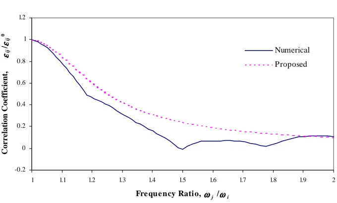
1. Comparison of numerically calculated eij values with those

obtained from existing formulations, ζi=0.01 and ζj=0.01 …………... 104 2. Comparison of numerically calculated eij values with those

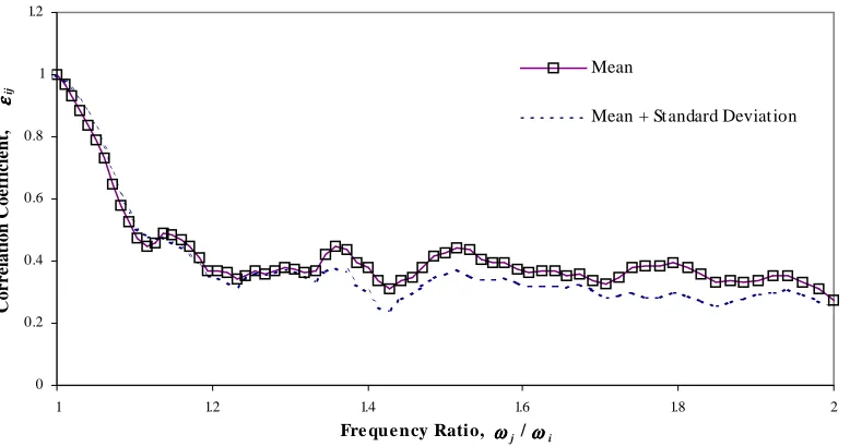
obtained from existing formulations, ζi=0.01 and ζj=0.07 ……….…... 104 3. Numerically calculated εij values using mean and mean plus one

standard deviation response in equation 15, ζi=0.01 and ζj=0.01 ….… 105 4. Numerically calculated εij values using mean and mean plus one

standard deviation response in equation 15, ζi=0.01 and ζj =0.07 .…... 105 5. εij/εij0 _{for modal responses with same algebraic sign,} ζ

i =0.01

and ζj =0.01 ……… 106

6. εij/εij0 _{for modal responses with same algebraic sign,} ζ

i =0.01

and ζj =0.02 ………. 106

7. εij/εij0 _{for modal responses with same algebraic sign,} ζ

i =0.01

and ζj =0.02 ……… 107

8. εij/εij0 _{for modal responses with same algebraic sign,} ζ

i =0.01

and ζj =0.07 ……….. 107

9. εij/εij0 _{for modal responses with same algebraic sign,} ζ

i =0.01

and ζj =0.10 ……… 108

10. εij/εij0 _{for modal responses with same algebraic sign,} ζ

and ζj =0.2 ……….. 108 11. εij/εij0 _{for modal responses with same algebraic sign,} ζ

i =0.02

and ζj =0.05 ………. 109

12. εij/εij0

for modal responses with same algebraic sign, ζi =0.02

and ζj =0.07 ……… 109

13. εij/εij0 _{for modal responses with same algebraic sign,} ζ

i =0.02

and ζj =0.10 ……… 110

14. εij/εij0 _{for modal responses with same algebraic sign,} ζ

i =0.05

and ζj =0.05 ……… 110

15. εij/εij0 _{for modal responses with same algebraic sign,} ζ

i =0.05

and ζj =0.07 ………. 111

16. εij/εij0 _{for modal responses with same algebraic sign,} ζ

i =0.05

and ζj =0.10 ………. 111

17. εij/εij0 _{for modal responses with same algebraic sign,} ζ

i =0.07

and ζj =0.07 ……… 112

18. εij/εij0 _{for modal responses with same algebraic sign,} ζ

i =0.07

and ζj =0.10 ………. 112

19. εij/εij0 _{for modal responses with same algebraic sign,} ζ

i =0.10

and ζj =0.10 ……… 113

20. εij/εij0 _{for modal responses with same algebraic sign,} ζ

i =0.01

and ζj =0.01 ………. 113

21. εij/εij0 _{for modal responses with same algebraic sign,} ζ

i =0.01

and ζj =0.07 ………. 114

22. εij/εij0

for modal responses with same algebraic sign, ζi =0.05

and ζj =0.07 ………. 114

23. εij/εij0 _{for modal responses with different algebraic sign,} ζ

i =0.01

and ζj =0.01 ………. 115

24. εij/εij0 _{for modal responses with different algebraic sign,} ζ

i =0.01

and ζj =0.02 ……… 115

25. εij/εij0 _{for modal responses with different algebraic sign,} ζ

i =0.01

and ζj =0.05 ………..….. 116

26. εij/εij0 _{for modal responses with different algebraic sign,} ζ

i =0.01

and ζj =0.07 ………..…….. 116

27. εij/εij0 _{for modal responses with different algebraic sign,} ζ

i =0.01

and ζj =0.10 ………..….. 117

28. εij/εij0 _{for modal responses with different algebraic sign,} ζ

i =0.02

and ζj =0.02 ………..………….. 117

29. εij/εij0 _{for modal responses with different algebraic sign,} ζ

i =0.02

and ζj =0.05 ………..……….. 118

30. εij/εij0 _{for modal responses with different algebraic sign,} ζ

i =0.02

31. εij/εij0 _{for modal responses with different algebraic sign,} ζ

i =0.02

and ζj =0.10 ……….. 119

32. εij/εij0 _{for modal responses with different algebraic sign,} ζ

i =0.05

and ζj =0.05 ……….. 119

33. εij/εij0

for modal responses with different algebraic sign, ζi =0.05

and ζj =0.07 ……….. 120

34. εij/εij0

for modal responses with different algebraic sign, ζi =0.05

and ζj =0.10 ……….. 120

35. εij/εij0 _{for modal responses with different algebraic sign,} ζ

i =0.07

and ζj =0.07 ……….. 121

36. εij/εij0 _{for modal responses with different algebraic sign,} ζ

i =0.07

and ζj =0.10 ……….. 121

37. εij/εij0 _{for modal responses with different algebraic sign,} ζ

i =0.10

and ζj =0.10 ……….. 122

38. Correlation Coefficient εij0_; ζ

i =0.01 ……….…….. 122

39. Correlation Coefficient εij0_; ζ

i =0.02 ……… 123

40. Correlation Coefficient εij0_; ζ

i =0.05 ………... 123

41. Correlation Coefficient εij0_; ζ

i =0.07 ……… 124

42. Correlation Coefficient εij0_; ζ

i =0.10 ……… 124

43. Correlation Coefficient εij0_; ζ

i =0.01 ……… 125

44. Correlation Coefficient εij0_; ζ

i =0.02 ………..…………. 125

45. Correlation Coefficient εij0_; ζ

i =0.05 ………..…..……... 126

46. Correlation Coefficient εij0_; ζ

i =0.07 ………..…..……… 126

47. Correlation Coefficient εij0

PART I

INTRODUCTION

INTRODUCTION

The seismic response of secondary systems depends, in addition to their uncoupled

dynamic characteristics, on the interaction with primary structures supporting them.

Considerable effort has been made in the past to develop procedures for evaluating

response of non-classically damped, coupled primary-secondary systems using their

uncoupled modal properties and design response spectra at the base of primary structure

directly. Responses obtained from such analyses are more accurate and often reduce the

conservatism in the design compared to a conventional analysis of uncoupled primary

and secondary systems. In general, the two uncoupled systems have different damping

characteristics, making the coupled system non-classically damped.

The non-classical nature of damping matrix makes the eigenvalues and

eigenvectors complex. Villavarde and Newmark (1980) developed a deterministic

formulation for non-classically damped systems starting with the complex frequencies

and mode shapes. They showed that the response for each complex mode shape and its

conjugate can be represented in two parts, one based on the relative displacement

spectrum and the other on the relative velocity spectrum. They assumed that the two

spectra are equivalent when expressed in the same units. This assumption does not hold

in the low and high frequency ranges. Also, they concentrated their efforts on secondary

systems, which are connected to the primary system at one or two points only.

Singh (1976) was among the first to present an alternative formulation based on

stochastic method. The method consists of developing a power spectral density function

system are used to obtain PSDF at any connecting degree of freedom (DOF), which in

turn would give the desired Instructure Response Spectra (IRS) at that DOF. However,

the process of generating an input response spectrum compatible PSDF is not unique. The

method also assumes that the ground motion is a stationary Gaussian process. This

assumption leads to overestimating the response in the low frequency range.

Der Kierighian et al. (1983) evaluated the response to a stochastic input. Unlike

Singh (1976), they modeled the earthquake as a white noise. The new method was an

improvement in that it accounted for interaction between the equipment and the structure,

and the correlation between the modes with closely spaced frequencies. However, other

problems inherent in the stochastic method remain. Igusa and Der Kieurighian (1985)

used the random vibration technique to develop an approximate method for the dynamic

analysis of multiply connected multi- degree-of-freedom secondary systems. This method

accounts for the interaction between primary and secondary systems, cross-correlation

between support motions, correlation between modal responses for stochastic input,

tuning between frequencies of the two systems, and the non-classical damping effect.

They also developed a modal combination rule for systems with non-classical damping

and closely spaced frequencies for stationary wide-band input. They used a perturbation

technique to derive closed form expressions for the complex modal properties of the

non-classically damped primary-secondary systems. However, their solution for the

eigenvalues and eigenvectors is correct only upto first order. Jaw and Gupta (1987) have

shown that the error in the eigenvalues and eigenvectors increases with the mass ratio

lightness of the secondary system in developing the approach. Singh and Suarez (1987)

proposed a different perturbation approach for evaluating eigenproperties of the

combined equipment-structure system. Through a rigorous analysis carried upto the

second order terms, the closed form expressions were derived for coupled frequencies,

mode shapes, and modal participation factors.

Gupta and Jaw (1986) developed an approximate method to obtain the coupled

frequencies, damping ratios, and mode shapes of the non-classically damped systems in

terms of the uncoupled modal properties of the classically damped primary and secondary

systems. They simplified the analysis by algebraically replacing the complex mode shape

by two real modal vectors. They also presented an alternate modal superposition method

for these real vectors. Gupta and Jaw (1986) further extended their formulation to the

response spectrum method. They also proposed a method for estimating the relative

velocity spectrum needed in the analysis.

Formulations proposed by Gupta and Jaw (1984) are based on the assumption that

the uncoupled modal properties of the primary and secondary systems are known for all

the modes. This is not practical for systems with large DOF. Gupta and Gupta (1999 a,b)

illustrated that a modal synthesis can give incorrect modal properties and seismic

response of non-classically damped coupled systems when all the modes of the

uncoupled primary and secondary are not included. They represented the effect of

missing mass contained in the truncated high frequency modes using residual modal

Gupta (1999) illustrated that the effect of non-classical damping is significant

when the uncoupled systems are tuned or nearly tuned and the modal mass ratios are

sufficiently small. He also illustrated that almost all the response in such systems comes

primarily from the response vectors associated with the relative velocity input and the

response vectors associated with the relative displacement input are negligible. Further,

Gupta and Gupta (1995) analyzed several real-life building-piping systems to show that

the coupled responses can be an order of magnitude less than the uncoupled responses

even when the modal mass ratios are extremely small. The method proposed by Gupta

(1992) and Gupta and Gupta (1998 a,b) is implemented in a computer program CREST

(1997), which is interfaced with the piping analysis program PIPESTRESS (1997) for

application to building-piping systems.

These computer programs have been validated by a comparison of the results

obtained from a modal time history analysis with those obtained from the corresponding

direct integration time history analysis. Similar comparison has also been made for the

results obtained from a response spectrum analysis. Other researchers have also

conducted similar verification studies (Der kieurighian 1983, Singh 1987). However, all

these studies use only simple representative systems and do not consider any real-life like

building-piping system. Further, the majority of simple systems considered in these

studies do not represent realistic coupled systems with significant effect of non-classical

damping as they have either high values of mass ratios or systems with detuned modes.

Recently, Brookhaven National Laboratory, under contract to US Nuclear Regulatory

various formulations for evaluating the seismic response of non-classically damped

coupled systems (USNRC 2000).

In the response spectrum method for evaluating the seismic response of structural

systems, the maximum modal responses are combined using an approximate formulation

for the modal correlation coefficient. A summary of various methods for combining

modal responses is given by Gupta (1992).

Rosenbleuth and Elorduy (1969) have given an expression for the correlation

coefficient by approximating the earthquake ground motion as a finite segment of white

noise and the modal response as completely damped periodic. Based on random vibration

theory, Der Kieurighian (1981) developed expressions for modal correlation coefficients

by considering earthquake excitations to be stationary white noise of infinite duration.

Under the assumption of stationarity for the response, Singh and Chu (1976) and Singh

and Mehta (1983) have presented the equations for superposition of modal responses in

response spectrum method, from which it is possible to write an equivalent expression for

the modal correlation coefficient.

In general, it has been found that the formulations based on the assumption of

stationarity underestimate the correlation coefficient. Many attempts have been made to

avoid this assumption. Rosenbleuth and Elorduy (1969) have approximated the

non-stationary transient nature of the response due to finite duration of the input earthquake

excitation by including a term representing the strong motion duration of the input. Gupta

and Cordero (1981) suggested modifications to the expression proposed by Rosenbleuth

Later, Gupta (1984) proposed another method for deriving the expression for

combination of modal responses in non-classically damped systems. The modal response

in non-classically damped system consists of two parts, one corresponding to the relative

displacement input and the other to the relative velocity input. Therefore, Gupta (1992)

proposed three different correlation coefficients, one for modal responses corresponding

to the relative displacement input, another for those corresponding to the relative velocity

input, and a third for cross correlation between the two types of modal responses. Similar

expressions have been proposed by Igusa and Der Kieurighian (1985). An important

observation made by Gupta (1992) is that total response in a particular mode is damped

periodic only in low frequency regions. The contribution of rigid part increases gradually

with increasing value of frequency and the response becomes completely rigid beyond

the rigid frequency of input motion. Gupta et al. (1996) presented a formulation to

separate the damped periodic and rigid parts of a modal response using rigid response

coefficient. Similar expressions for rigid-response coefficient have been proposed by

Lindely and Yow (1980). However, their study is heuristic in nature and gives incorrect

values in the low frequency region (below the peak of input spectrum). Recently,

USNRC (1999) conducted a benchmarking study to compare and evaluate the validity of

various methods.

Consideration of only the maximum modal responses in a response spectrum

method makes it a design method which cannot reproduce the results obtained from a

time history analysis on a one-to-one basis. Instead, the results from the two methods

the mean and the standard deviation of responses obtained from multiple time history

analyses should be close to the corresponding values obtained from the response

spectrum method. As pointed out in Gupta (1992), a time history analysis should be

preferred over a response spectrum analysis if the input time history of the ground motion

is known. However, this is not the case in design, as the input time histories for future

earthquakes are not known a-priori. For design purposes, earthquake input is defined as a

response spectrum corresponding to a specified level of non-exceedence probability. The

non-exceedence probability ranges from 0.50 for ordinary structures to 0.84 for critical

industrial facilities such as nuclear power plants. Such a definition of input design

response spectrum ensures that the modal responses have the same non-exceedence

probability as that of the design spectrum. However, the total response obtained after

combining individual modal responses may not necessarily correspond to the same

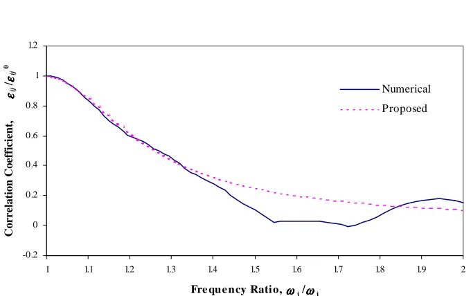
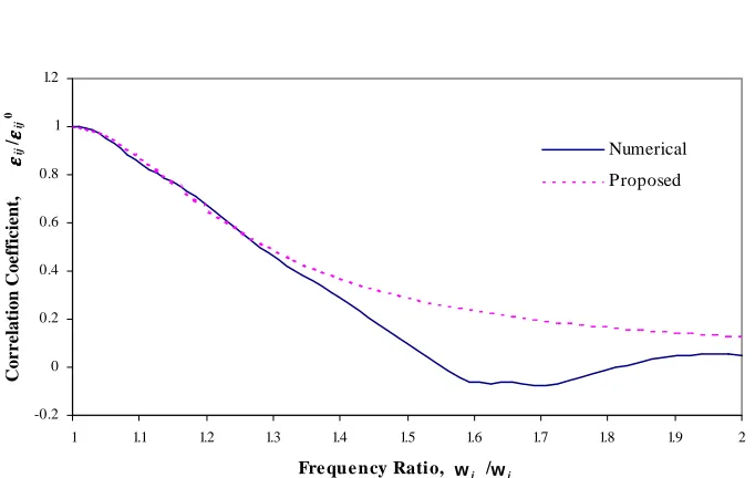
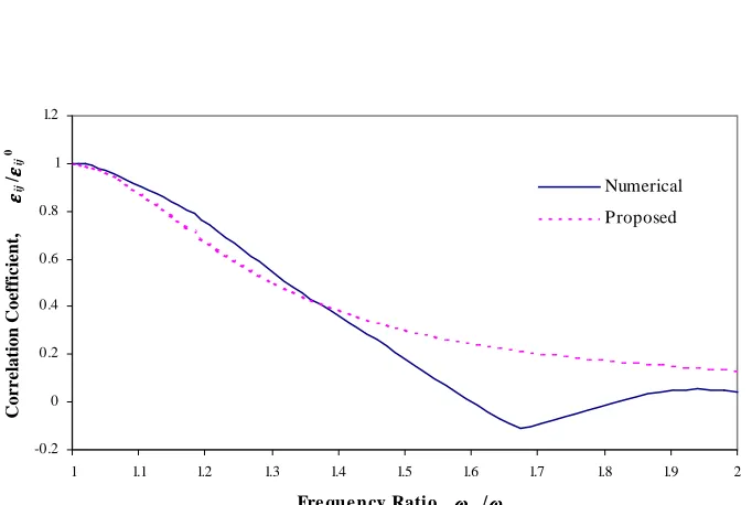
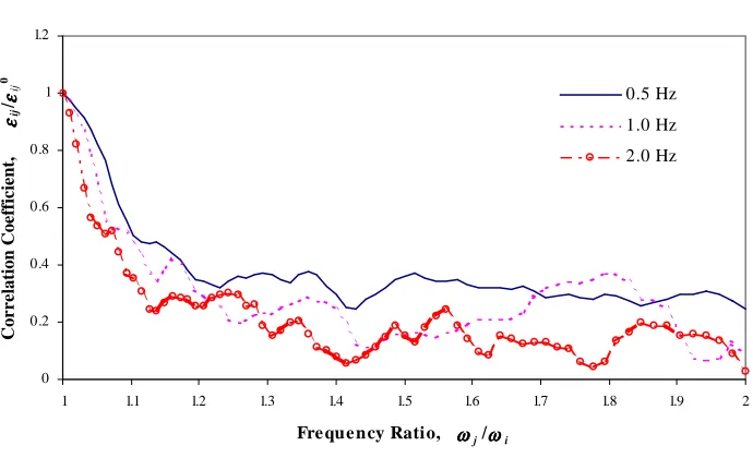
non-exceedence probability. In this paper, a numerical study is presented to illustrate that the

modal correlation coefficients evaluated using the existing formulations can be

significantly less than those needed for evaluating design response corresponding to a

specified level of non-exceedence probability.

OBJECTIVE

The specific tasks required to achieve the objective of this study are:

• Modify computer program CREST/PIPETSRESS to create a new program

CREST-TH which performs a time-wise modal superposition analysis of simple as well as

• Coordinate with Brookhaven National Laboratory (BNL) to develop several simple

but realistic coupled systems for validation of CREST and CREST-TH, study the

effects of mass interaction, tuning of modes, non-classical damping, multiple support

excitation, and high frequency modes using these systems.

• Consider two real-life building-piping systems and perform modal superposition time

history analyses for each simple and real-life like coupled system. Compare the

responses with those evaluated by BNL from a direct integration time history

analysis.

• Study differences in non-classical and composite modal damping.

• Evaluate responses using response spectrum analysis for each system. Compare the

responses with those evaluated from time history analysis.

• Study methods for combining modal responses.

• Develop new formulations for modal correlation coefficients that are consistent with

the evaluation of design response in a response spectrum method.

ORGANIZATION

This dissertation consists of primarily three manuscripts that the authors plan to submit

for publication in the peer-reviewed journals. Part I of the dissertation provides an

introduction and detailed discussion on the existing literature for evaluating seismic

response of non-classically damped primary-secondary systems as well as for evaluating

modal correlation coefficients. The first and second manuscripts, Parts II and III of the

validation of the formulations for evaluating the seismic response of nonclassically

damped coupled systems. An extensive discussion is presented on the results obtained

from modal superposition time history analyses as well as the response spectrum analyses

of simple and real-life like building-piping systems. Part II also provides a detailed

discussion on the significance of non-classical damping in primary-secondary systems

and on the differences between the non-classical, classical, and composite modal

damping. In part III, a detailed discussion is provided on the numerical and modeling

differences that can occur in real-life like building-piping systems. Effect of these

inaccuracies on the dynamic characteristics of the coupled system is also illustrated.

The manuscript given in Part IV of this dissertation provides a discussion on the

existing formulations for modal correlation coefficients and the limitations of these

formulations in the evaluation of design response corresponding to a specified level of

non-exceedence probability. A numerical study is presented to illustrate that the modal

correlation coefficient evaluated using the existing formulations can be significantly less

than those needed for evaluating the design response. An empirical study is used to

propose a new definition for the modal correlation coefficient that is consistent with the

evaluation of design response in response spectrum method. Finally, the summary and

conclusions of this study and the recommendations for future studies are presented in Part

REFERENCES

Der Kieurighian, A. (1981). “A Response Spectrum Method for Random Vibration Analysis of MDOF Systems”, Earthquake Engineering and Structural Dynamics, Vol. 9, pp. 419-435.

Der Kieurighian, A.,Sackman, J. L. and Nour-Omid, B. (1983) “Dynamic Analysis of Light Equipment in Structures: Response to Stochastic Input”, Journal of

Engineering Mechnics, ASCE, Vol. 109, pp. 90-95.

DST (1997), DST/PIPESTRESS User’s Manual. DST Computers Services of Geneva, Switzerland, Version 3.4.09.

Gupta, A. (1999), “Significance of Nonclassical Damping in Coupled System Analysis”, Proceedings, 15th Structural Mechanics in Reactor Technology Conference, 1/K4-A8, Seoul.

Gupta, A. K. (1992), Response Spectrum Method in Seismic Analysis and Design of Structures, CRC Press.

Gupta, A. K., Hassan, T. and Gupta, A. (1996). “Correlation Coefficients for Modal Response Combination of Non-classically Damped Systems”, Nuclear Engineering and Design, Vol. 165, pp. 67-80.

Gupta, A. and Bose, M. K. (1997). CREST, A Computer Program for Coupled

Response Spectrum Analysis of Secondary Systems Interfaced with PIPESTRESS, User’s Manual, Report C-NPP-SEP 9/95, Department of Civil Engineering, NC State University, Raleigh, North Carolina.

Gupta, A. and Gupta, A. K. (1998a). “Missing Mass Effect in Coupled Analysis I: Complex Modal Properties”, Journal of Structural Engineering, ASCE, Vol. 124,

pp. 490-495.

Gupta, A. and Gupta, A. K. (1998b). “Missing Mass Effect in Coupled Analysis II: Residual Response”, Journal of Structural Engineering, ASCE, Vol. 124,

pp. 496-500.

Gupta, A. and Gupta, A. K. (1995). “Applications of New Developments in Coupled Seismic Analysis of Piping systems”, 13th Structural Mechanics in Reactor Technology Conference, K7/3, Stuttgart.

Gupta, A. K. and Jaw, J. W. (1986). “Coupled Response Spectrum Analysis of Secondary Systems Using Uncoupled Modal Properties”, Nuclear Engineering and Design, Vol. 92, pp. 61-68.

Igusa, T. and Der Kieurighian, A. (1985).”Dynamic Response of Multiply Supported secondary Systems”, Journal of Engineering Mechanics, ASCE, Vol. 111, pp. 20-41.

Jaw, J. W. and Gupta, A. K. (1987) “Seismic Response of Multiply Connected MDOF Secondary Systems”, Department of Civil Engineering., NC State University.

Lindley, D.W. and Yow, J. R. (1980). “Modal Response summation for Seismic Qualification”, 2nd ASCE Speciality Conference on Civil Engineering and Nuclear

Power, Vol. VI, Paper 8-2, Knoxville, TN.

Rosenbleuth, E. and Elorduy, J. (1969). “Response of Linear Systems to Certain Transient Disturbances”, Proceedings, 4th World Conference on Earthquake Engineering. A-1, pp. 185-196.

Singh, M. P. and Chu, S. L. (1976). “Stochastic Considerations in Seismic Analysis of Structures”, Earthquake Engineering and Structural Dynamics, Vol. 4, pp. 295-307.

Singh, M. P. and Chu, S. L. (1976). “Stochastic Considerations in Seismic Analysis of Structures”, Earthquake Engineering and Structural Dynamics, Vol. 4, pp. 295-307.

Singh, M. P. and Mehta, K. B. (1983). “Seismic Design Response by an Alternative SRSS Rule”, Earthquake Engineering and Structural Dynamics, Vol. 11, pp. 771- 183.

Singh, M. P. and Suarez, L. E. (1987). “Perturbed Coupled Eigenproperties of Non- Classically Damped Primary Structure and Equipment Systems.” Journal of Sound and Vibration, Vol. 116, pp. 199-220.

Villavarde, R. and Newmark, N. M. (1980). “Seismic Response of Light Attachments to Buildings”, Structural Research Series, No. 469, University of Illinois, Urbana.

USNRC (1999). “Reevaluation of Regulatory Guidance on Modal Response

Combination Methods for Seismic Response Spectrum Analysis”, NUREG/CR-6645, US Nuclear Regulatory Commission/Brookhaven National Laboratory, Eds. Morante, R. and Wang, Y..

USNRC (2000). “Benchmark Program for the Evaluation of Methods to

PART II

VERIFICATION OF METHODS FOR EVALUATING

SEISMIC RESPONSE OF NON-CLASSICALLY DAMPED

PRIMARY-SECONDARY SYSTEMS:

SIMPLE COUPLED SYSTEMS

VERIFICATION OF METHODS FOR EVALUATING SEISMIC

RESPONSE OF NON-CLASSICALLY DAMPED

PRIMARY-SECONDARY SYSTEMS:

SIMPLE COUPLED SYSTEMS

Abhinav Gupta, Mrinal K. Bose, Ajaya K. Gupta

Center for Nuclear Power Plant Structures, Equipment and Piping, North Carolina State University Campus Box 7908, Raleigh, NC 27695-7908, USA

ABSTRACT: Results from a verification study of formulations for evaluating the

seismic response of non-classically damped primary-secondary systems are presented. A

parametric study is concluded in which three different configurations of simple

representative systems are considered. Responses obtained from modal superposition

time history analyses as well as response spectrum analyses are compared with the

corresponding responses obtained by Brookhaven National Laboratory from the direct

integration time history analyses. Modal superposition time history analyses results and

direct integration time history analyses results are almost identical. The mean and

standard deviation of responses from response spectrum analyses are close to the

corresponding values evaluated using direct integration time history analyses. It has been

combination of modal tuning, modal mass ratio and the difference in the modal damping

ratios. In addition to the verification results, a detailed discussion is also presented on the

significance of non-classical damping. It is shown that the effect of non-classical

damping is significant in systems that have nearly tuned modes and sufficiently small

values of modal mass ratios. It is also illustrated that composite modal damping is an

alternate form of classical damping that can give incorrect responses in non-classically

damped systems

INTRODUCTION

The current practice of calculating seismic response is to perform the analysis of primary

system (buildings) and secondary systems (equipment and piping) separately. The

seismic response of secondary systems depends, in addition to their uncoupled dynamic

characteristics, on the interaction with the primary structures supporting them. Seismic

analysis of a coupled primary-secondary system gives responses that are more accurate

and are often less than those calculated from an uncoupled analysis (Gupta 1992). Unlike

the conventional uncoupled analysis, a coupled system analysis accounts for the effects

of mass interaction, tuning between the modes of the uncoupled systems, non-classical

damping, and correlation between inputs at various supports of a multiply supported

piping system. Considerable effort has been made in the past to evaluate the response of

non-classically damped coupled primary-secondary systems using their uncoupled modal

(Burdisso and Singh 1987; Igusa and Der Kieurighian 1985; Gupta and Gupta 1998;

Villavarde and Newmark 1980).

Almost all the existing formulations have been verified by a comparison of the

results obtained from a modal superposition time history analysis of the coupled system

with the corresponding results obtained from a direct integration of the equation of

motion. However, these verification studies considered only simple representative

primary-secondary systems. No real-life-like coupled system such as building-piping was

used in these studies. Recently, Brookhaven National Laboratory (BNL) conducted a

benchmark program for the US Nuclear Regulatory Commission to evaluate and verify

the various methods of calculating seismic response in non-classically damped coupled

primary-secondary systems (USNRC 2000). A parametric study was conducted and a

total of 62 cases were considered. Three different configurations of simple systems and

one configuration of real-life-like building-piping system were considered to generate

these test cases by varying key parameters including the floor mass ratio. Not only were

the results obtained from modal superposition time history analyses compared with the

results obtained from a direct integration of the equation of motion, the results obtained

from the corresponding response spectrum analyses were also considered for verification

purposes.

As stated earlier, a coupled system analysis can account for the effect of

non-classical damping. The coupled system becomes non-non-classically damped when the

damping characteristics of the uncoupled primary and secondary systems are different.

to the complex eigenvectors and eigenvalues can be represented using two real vectors,

one corresponding to the relative displacement input and the other to the relative velocity

input (Gupta 1992). The response corresponding to the relative velocity input exists only

when the coupled system is non-classically damped and is null when it is classically

damped. Gupta (1999) has shown that the effect of non-classical damping is significant

only when the two uncoupled systems are tuned or nearly tuned and the modal mass

ratios are sufficiently small. Typical values for the modal mass ratios in actual

building-piping systems have been found to be on the order of 0.0001 or lower. Even though the

various existing formulations account for this effect, the simple systems used in the

verification studies are not representative of the systems that have significant effect of

non-classical damping due to the following reasons. The simple systems considered for

verification purposes in the earlier studies have either relatively higher values of mass

ratios or systems with detuned modes. Consequently, these simple systems do not

represent coupled systems that have significant effect of non-classical damping.

In the study conducted by BNL, an attempt was also made to compare the results

obtained by considering the non-classical nature of the damping matrix to those obtained

by using composite modal damping for the coupled system (Bose and Gupta 2000).

However, the results obtained from the two types of damping models were compared

only for the response spectrum method of analysis. Results corresponding to a time

history analysis with composite modal damping, either by modal superposition or by

direct integration, were not considered. Based on the results obtained from response

damping characteristics give close results. Even though large differences in the results

obtained from the two methods of modeling damping characteristics were noticed for

real-life like building-piping systems, these differences were attributed to the differences

in stiffness characteristics of the building-piping models between the two sets of

analyses.

In the present paper, a discussion of the results obtained from our participation in

the benchmark program conducted by BNL is provided and two additional independent

topics encountered but not completely addressed in the validation study conducted by

BNL are discussed. First, differences between non-classical, classical and composite

modal damping are studied by comparison of time history analysis results in simple

systems. Next, possible reasons for numerical and modeling differences in real-life like

building-piping system considered in the benchmark program are identified and their

effect on the dynamic characteristics of the coupled system is illustrated. The latter is

given in a companion paper (Bose et al. 2001).

COUPLED EQUATION OF MOTION

The equation of motion for an N-DOF coupled primary-secondary system can be written

as

g

u

_{CU KU MUb}

U

M ++++ ++++ ====−−−− (1)

where, M, C, and K are the mass, damping and stiffness matrices, respectively of the

coupled system; U is the displacement vector relative to the fixed base; Ub is the static

unit displacement in the direction of the earthquake, and u_g is the ground acceleration. These matrices and vectors can be expressed in terms of the matrices and vectors of the

primary and secondary systems, denoted by subscripts p and s, respectively.

þþþþ ýýýý üüüü îîîî íííí ìììì ==== þþþþ ýýýý üüüü îîîî íííí ìììì ==== úúúú úúúú ûûûû ùùùù êêêê êêêê ëëëë éééé ++++ ==== úúúú úúúú ûûûû ùùùù êêêê êêêê ëëëë éééé ++++ ==== úúúú ûûûû ùùùù êêêê ëëëë éééé ==== bs bp b s p s sp ps s p p s sp ps s p p s p U U U ; U U U ; K K K K K K C C C C C C ; M O O M M (2)

The matrices Ks_pand Cs_p are the stiffness and the damping contributions of the secondary

system with respect to the primary system's connecting degrees of freedom. In the above

equation, the displacement vector is expressed relative to the fixed base of the primary

system. Gupta and Gupta (1998a) presented a transformation in which the secondary

system DOF are expressed relative to the primary system connecting DOF. The new set

of DOF for the coupled system, U , can be evaluated as

U T U U I U O I U U U s p sp s p ₌ þ ý ü î í ì ú û ù ê ë é = þ ý ü î í ì

= (3)

where, U_p ≡≡≡≡U_p, and the matrix Usp contains secondary system displacement vectors

each of which represents the static deformation shape of the secondary system when the

primary system degrees of freedom undergo a unit displacement. Only those vectors that

correspond to the primary system connecting DOF contain non-zero values. Substituting

Eq. (3) into Eq. (1) and pre-multiplying by T T, the transformed equation of motion is

given by

g

bu

_{CU KU MU}

U

EIGENVALUE PROBLEM

The equation of motion for the coupled system can be transformed further using the mode

shapes of the uncoupled primary and secondary systems (Gupta and Gupta 1998a; Igusa

and Der Kiureghian 1983; Gupta and Jaw 1986). It is assumed that the uncoupled

primary and the uncoupled secondary systems are classically damped. Therefore, the

damping matrices Cp and Csare diagonalized when they are pre- and post-multiplied by

the respective undamped modal matrices. Such systems are called classically damped.

However, when the modal damping ratios of the two systems are unequal, the combined

damping matrix C would be no longer diagonal when pre- and post-multiplied by the

undamped modal matrix of the coupled system. The combined system, therefore,

becomes non-classically damped. Let subscript i and other lower case letters denote the

primary system modes and the subscript α and other Greek letters denote the secondary

system modes. Let the ith mode shape of the uncoupled primary system be φφφφpi and the αth

mode shape of the uncoupled secondary system be φφφφsα such that φφφφT_piM_pφφφφ_pi ====1 and

1

====

sα

s T sαM φφφφ

φφφφ . In terms of the uncoupled mode shapes we can write

þþþþ ýýýý üüüü îîîî íííí ìììì úúúú ûûûû ùùùù êêêê ëëëë éééé ==== ==== s p s p X X Φ 0 0 Φ X Φ

U (5)

Substituting Eq. (5) in Eq. (4) and premultiplying by ΦT , we get

g T _u b U M X K~ X C~ X

M~ ++++ ++++ ==== −−−−ΦΦΦΦ (6)

The various matrices and vectors in the above equation can be written in terms of

ú ú û ù ê ê ë é ₊ = ú ú û ù ê ê ë é = ú ú û ù ê ê ë é ₊ = s s p p s p s sp ps s p p K O O K K K C O O C C M M M M M M _~ ~ ~ ~ ; ~ ~ ~ ; ~ ~ ~ ~ ~ ~ (7a) þ ý ü î í ì ú û ù ê ë é − = þ ý ü î í ì = = − bs bp sp bs bp b b _U U I U O I U U U T U 1 (7b)

When the base of primary system undergoes a unit deflection in the direction of

earthquake, no relative displacement exists between the two uncoupled systems, giving

0

====

bs

U . Further, we can express the various matrices in the above equations as

M~_p ++++M~_ps ====I++++Φ_pTU_spT M_sU_spΦ_p (8a)

M~_ps ==== M~_spT ====ΦT_pUT_spM_sΦ_s (8b)

M_s=I

~

(8c) C~_p ====ΦT_pC_pΦ_p (8d)

C~_s ====ΦT_s C_sΦ_s (8e)

K~_p++++K~_ps ====ΦT_p K_pΦ_p++++ΦT_p

((((

))))

M~_ij ==== 1 ++++ φT_pi U_spT M_s U_sp φ_pi , i ==== j (9a)

==== φφφφ_piT U_spT M_s U_sp φφφφ_pj , i ≠≠≠≠ j (9b)

j i

ζ ω

j i ≠≠≠≠

====0, (9d)

K~_ij ==== ω2_pi ++++ ∆ω_pij2 , i ==== j (9e)

==== ∆ω2_pij, i ≠≠≠≠ j (9f)

∆ω_pij2 ==== φφφφT_pi

((((

))))

where, ∆ω2_pijrepresents the effect of static constraint offered by the secondary system on the primary system. The corresponding term in the transformed damping matrix is

neglected. Matrix M~_ps has elements that can be defined as

M~_iα = φ_piTU_spT M_sφ_sα =r_i1_α/2 (10)

in which riα is the modal mass ratio that represents the ratio of secondary system mass

participating in the αth uncoupled mode to the primary system mass participating in its

own ith uncoupled mode. It is a parameter that describes the interaction between the modes of two uncoupled systems. For a SDOF primary and SDOF secondary system, its

value is equal to the ratio of secondary to primary system mass. The various elements of

matrices M~_s, C~_s, and K~_scan be written as

β α αβ ==== , ==== ~

1

M (11a)

β α ≠≠≠≠

==== 0, (11b)

β α ζ

ω α α

αβ ==== 2 , ====

C _s s

~

(11c)

β α ≠≠≠≠

==== 0, (11d)

β α ω α

αβ ==== s2 , ====

β α ≠≠≠≠

==== 0, (11f) If the eigenvalues of the coupled system are denoted by λ, the free vibration equation of

motion corresponding to Eq. (6) becomes

K*X ====O; K* ====K~++++λC~++++λ2M~ (12)

For non-classically damped systems, the eigenvalue problem given by the above equation

gives complex eigenvalues and eigenvectors together with their conjugates.

COUPLED SYSTEM RESPONSE

The complex eigenvalue in the ith coupled mode λi and its conjugate λ_i give the coupled

modal frequency ωi and the damping ratio ζi. Each complex eigenvector and its conjugate

gives two real modal vectors, Ψ_id and Ψ_iv, (Gupta and Gupta 1998b)

((((

))))

((((

))))

Re Ψ , Ψ Ψ

Ψ v

i d

i ==== −−−−2 ==== −−−−2 (13a)

Ψ_i====ΦX_i (13b)

in which,

==== X_iT Γ , ΓT ====

[[[[

]]]]

i

a

F 1 (14a)

a_i = 2λ_i X_iT M~ X~_i + X_iT C~ X_i (14b) Γ_pT =

[

]

[

]

_spT _{s bs sα}T _{s bs}

T p bp p T

p M U φ U M U φ M U

φ + =

= j j sα

pj γ

where φ_pjand φ _sα are mass normalized mode shapes of the uncoupled primary and

secondary system in the jth and αth modes, respectively.

TIME HISTORY ANALYSIS

For an acceleration time history input, the coupled response can be calculated either by

direct integration of the coupled system equation of motion i.e. Eq. (1). Alternatively, a

modal superposition may be used as follows

i i N i N i N i z z v i d i v i d i

i U U Ψ Ψ

U

U =

å

å

å

= =

=1 1 1

(15)

in which z_i is the relative displacement and z_i the relative velocity of an equivalent SDOF system and can be calculated from

g i 2 i i i i

i ωζ z ω z u

z ++++ 2 ++++ ==== −−−− (16)

RESPONSE SPECTRUM ANALYSIS

For design purposes, earthquake input is defined in terms of a response spectrum and not

an acceleration time history. In response spectrum method of analysis, the modal

responses are calculated as

v Di i d

Di ω S

S v i v i d i d

i Ψ ; U Ψ

U ==== ==== (17) where, S_Did and S_Div are the spectral displacements in coupled mode i. Superscripts d and v

denote that the spectral values correspond to the relative displacement and the relative

velocity spectra, respectively. Conventionally, the response spectrum is defined as that

velocity is not calculated and therefore, not available. A method to evaluate spectrum

curve corresponding to the relative velocity from the relative displacement spectrum is

given in Gupta et al. (1996). However, if the earthquake time history is known, both the

spectrum curves can be calculated directly by integrating Eq. (16). In this study, the

earthquake inputs are defined in terms of acceleration time histories. Therefore, both

spectra are evaluated directly from the time history at exact frequency and damping ratio

values for each mode. The modal responses in the response spectrum method are then

combined according to the method proposed by Gupta et al. (1996).

((((

))))

å

å

å

å å

å

å

å

ijR R ε R R 2µ R R

ε

R

1 1

2 (18)

in which R represents a response quantity of interest and

d j d i d ij d j d i d

ij α α ε α α

ε = {[1− ( )2][1−( )2]} + (19a)

v j v i v ij v j v i v

ij α α ε α α

ε = {[1−( )2][1−( )2]} +

(19b) ij v j d i

ij α α µ

µ = {[1−( )2][1− ( )2]} (19c)

where, ε_ijd ,ε_ijv and µ_ij are the modal correlation coefficients whereas α_idand α_ivare the

rigid response coefficients. These coefficients are described in detail in Gupta et al.

(1996). However, it should be noted that 0≤α_id,v ≤1. Gupta et al. (1996) illustrate that

in the low frequency region (fi less than a key frequency f1d) the response is completely

frequency fr) the response is completely rigid, i.e. α_id,v =1. For modes that have

frequencies in the intermediate frequency region ( f₁d ≤ f_i ≤ f_r), both the periodic and the rigid parts contribute significantly to the response. Values of f₁dand fr for various

input ground motions are evaluated in Gupta et al. (1996).

DAMPING MATRIX OF THE COUPLED SYSTEM

As stated earlier, it is assumed that the uncoupled secondary system is classically

damped, i.e.

[

]

T s s

s

ω

diag( 2 _αζ _α) = Φ C_sΦ (20)

in which ωsα and ζsα are the circular frequency and modal damping ratio, respectively, in

the αth uncoupled secondary system mode. The secondary system damping matrix

relative to its own fixed base, C_s, can be calculated using the undamped modal matrix ΦΦΦΦs

and the mass matrix Ms of the uncoupled secondary system.

[

]

) 2

( −

−

= T _{s s s}

s diag ω Φ

Φ

C_{s α}ζ _α (21)

Since Φ_sTM_sΦ_s = I , we can write

s

sΦ Φ Φ M

M

Φ_s−T = _{s s}−1 = _sT

; (22)

Therefore,

[

]

T s s

s

s M Φ Φ M

For developing the damping matrix of the coupled system, we need to express the

secondary system damping matrix relative to the fixed base of primary system and not its

own fixed base. This can be done by using the transformation developed earlier.

U Q U T U ₌₌₌₌ −−−−1 ₌₌₌₌

ú ú û ù ê ê ë é − − = = s sp s T sp sp s T sp s T t s C U C C U U C U Q C Q C

s (24)

The transformed matrix C_st is of order (NT × NT) where NT is the total number of DOF

for the coupled system (equal to the primary system DOF plus the secondary system

DOF). The primary system damping matrix Cp relative to its own base, can now be

assembled with matrix C_st to obtain the total damping matrix of the non-classically

damped coupled system. The primary system damping matrix Cp can be evaluated using

the same procedure as for the secondary system, i.e.

[[[[

]]]]

T p p

p

p M Φ ( ) Φ M

C ==== diag 2ω_pi S_pi (25)

in which ωpi and ζpi are the circular frequency and modal damping ratio of the ith

uncoupled primary system mode. Damping matrix of the coupled system can now be

DESCRIPTION OF BENCHMARK PROBLEMS: SIMPLE SYSTEMS

Three different configurations of simple non-classically damped primary-secondary

systems, shown in Figs. 1-4, were considered for performing a parametric validation

study in USNRC (2000). All the values given in this figures and the present paper have

been converted from US customary units to SI standard units. The primary system in all

the three configurations is a five degree-of-freedom shear building with uniform

distribution of story stiffness and floor mass. The first configuration is representative of a

simple equipment modeled as a four-degree-of-freedom secondary system that is

supported on the 4th floor of the primary system. The second configuration represents a six degrees of freedom piping system supported at multiple primary system floors i.e.

2nd,3rd and 4th floors. The third configuration consists of a six-degree-of-freedom

secondary system that is not only supported at multiple primary system floors i.e. 3rd and 4th, but also directly on the ground. The parametric study was conducted by a variation in four different quantities: (1) secondary system floor mass, (2) secondary system story

stiffness, (3) secondary system damping ratio, and (4) input ground motions. These four

quantities were considered to study the effects of variation in modal mass ratio, tuning

between the modes of two uncoupled systems, non-classcial damping, and characteristics

of input motion, respectively. A total of fourteen cases were considered for each coupled

system configuration that included four cases for mass ratio variations, five for frequency

ratio variations, three for damping ratio variations, and seven for different input ground

motions. Table 1 describes the characteristics for each of these fourteen cases. The