PARAMETER ESTIMATION USING AGGREGATE DATA

(1)

Parameter Estimation Using Aggregate Data

H. T. Banks

1

, Annabel E. Meade

1

, Celia Schacht

1

, Jared Catenacci

2

, W. Clayton

Thompson

3

, Daniel Abate-Daga

4

, and Heiko Enderling

4

1

_{Center for Research in Scientific Computation, N. C. State University, Raleigh, NC}

2

_{The Johns Hopkins University Applied Physics Laboratory, Laurel, MD}

3

_{SAS Institute, Cary, NC}

4

_{H. Lee Moffitt Cancer Center, Tampa, FL}

July 29, 2019

Abstract

In biomedical/physiological/ecological experiments, it is common for measurements in time series data to be collected from multiple subjects. Often it is the case that a subject cannot be measured or identified at multiple time points (often referred to as aggregate population data). Due to a lack of alternative methods, this form of data is typically treated as if it is collected from a single individual. As we show by examples, this assumption leads to an overconfidence in model parameter (means, variances) values and model based predictions. We discuss these issues in the context of a mathematical model to determine T-cell behavior with cancer chimeric antigen receptor (CAR) therapies where during the collection of data cancerous mice are sacrificed at each measurement time.

Key Words: uncertainty quantification, parameter estimation, CAR T cancer therapy

(2)

1 Introduction

Recently there has been increased awareness that many authors incorrectly treat aggregate or population level data as individual data. This is especially prevalent in biomedical and ecological applications where often the data is collected over several generations of those being observed or the collection of the data requires sacrifice of the objects – cells, animals or species, etc.– being observed. This is also frequently the case in electromagnetic interrogation where it is impossible to excite a single individual (electron). (See additional discussions in [7,10].) As explained in [3], this can, and often does, lead to confusion and incorrect analyses related to inter-individual and intra-individual variability in the case of even simple growth models where one can estimate mean growth rates correctly while failing to correctly determine the variances. Recent authors [2, 14] have encountered related problems in the context of employing delay differential equations requiring bi-Gaussian distributions describing growth and death of species of pests.

2 Logistic Growth and Improperly treating the Data as Individual

Data

Common to many PK/PD models is the notion of a saturation limit for a quantity of interest. For example, the saturation of drug/chemical concentration, the maximum size of tumor growth, or the saturation of a population of cells. Frequently, this limiting behavior results in a S-shaped curve, which can be described by a sigmoid, Hill, Gompertz, logistic, or one of several other functions.

Here we use, to demonstrate our ideas, the system with the solution to the (deterministic) logistic equation

dx

dt(t) =rx(t)

1−x(t)

K

, x(0) =x0. (1)

We begin by exploring potential pitfalls when disregarding the fact that the data is indeed aggregate data, which, again, we emphasize is a very common assumption made in biomedical/ecological modeling literature. Consider a standard experimental set up where the data with nttotal number of data points,y={yj}nj=1t ,

is collected by only collecting a single sample from a new subject at each sampling time. We generate an example data set with x0 = 10, K = 100, where the growth rate rwas drawn from a normal distribution

with mean 2 and variance 0.2, and then a noise level ofσ2

was added to each observation. This data set is

depicted in the upper left figure of Figure 1.

Since here, we wish to disregard the fact that the measurements are collected from different individuals and instead assumed that the observations are collected from a single individual over time, we arrive at the standard statistical model given by

yj =x(tj;θ) +j (2)

wherej is the measurement error andθ are the unknown parameters. In actual fact the data is aggregate

and given by

yij =xi(tj;θi) +ij (3)

for a correct model

dxi

dt (tj) =rixi(tj)(1− xi(tj)

(3)

from a single individual over time, i.e., individual longitudinal data.. We remark that this difference is, in fact, an example of model discrepancy (also referred to as model mispecification in the literature), and the discrepancy is due to the fundamental difference between the modeling assumptions of how the data is collected and how the data is actually generated experimentally. Thus, one possible approach, which we do not explore in this work, is to attempt to account for this model discrepancy in order to arrive at calibrated parameters for which the associated uncertainty agrees with the distributions of the individual parameters. Bayesian estimation is a powerful tool for uncertainty analysis, and here we will illustrate that even a Bayesian procedure leads to false conclusions if one assumes that the data is collected from a single individual when in reality the data is aggregate data. Through the means of a Bayesian estimation, we will estimate the unknown parametersθ= (r, x0, K)T in the logistic model (1). The prior density is denoted by

π0(θ), which we take as a uniform prior, and we further assume that the measurement errors are independent

and identically distributed with a normal distribution having mean 0 and varianceσ2

. With this assumption

the likelihood function is given by

π(y|θ) = 1 (2πσ2

)(nt/2)

exp{− 1

2σ2

nt

X

j=1

(yj−x(tj;θ))2} (5)

wherex(tj;θ) is the solution to the logistic equation (1). Then the posterior density can be obtained through

π(θ|y) =π(y|θ)π0(θ)

π(y) =

π(y|θ)π0(θ)

R

Rpπ(y|θ)π0(θ)dθ

. (6)

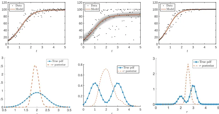
The posterior density was approximated using the delayed rejection adaptive Metropolis (DRAM) algo-rithm [19]. In Figure 1 (upper left), we present the model fit to a data set which was generated with the measurement error varianceσ2= 1. The mean parameters were found to ber= 1.9562,x0= 11.0010, and

K= 97.8998, and we see that we are able to estimate the mean value of the growth rate, the initial condi-tion, and the carrying capacity with reasonable accuracy. However, the approximate posterior density for the growth raterdoes not represent the true density, as can be seen in Figure 1 (lower left). In fact, we severely underestimate the variance of the growth parameter r, which was estimated to be V ar[π(r|y)] ≈ 0.0247. This is because the posterior density represents the certainty that the given values of r describe the data set. In this framework, there is no way to distinguish between the variance due to the intrinsic variability of the growth rate and the measurement noise. The result is an (unjustifiably) high level of confidence in the parameter estimate ofr, which, in this case, represents the mean of the true distribution, with no indication that we are not capturing the inherent variability in the system. We also show the 95% prediction interval, represented by the shaded region about the model fit in Figure 1 (upper left). Clearly the prediction in-terval grossly underestimates the variance observed in the simulated data measurements. This is a further indication of how the overconfidence we have obtained in our parameter estimates can adversely affect the predictive capabilities in a model analysis.

In a second example we used a Bi-Gaussian distribution to generate data as in the first example above. The true distribution for the growth rate in the logistic model is a Bi-Gaussian (µ1 = 1, µ2= 3 and equal

variancesσ2

1 =σ22=.2). We then estimated the growth rate using Bayesian estimation and the posterior for

the growth rate is uni-modal as depicted in the middle graph in Figure 1 with the mean being about 2. We see the data fit to model in the upper middle image of Figure 1. The a priori used in a Bayesian estimation procedure as described above was again a uniform distribution.

(4)

0 1 2 3 4 5 0 20 40 60 80 100 120

0 1 2 3 4 5 0.2

0.4 0.6 0.8

Figure 1: Simulated aggregate logistic data and corresponding Bayesian estimation results (top row) along with the true and estimated posterior PDFs (bottom row). Aggregate data sets are simulated by letting the growth rate parameterrbe drawn from a normal distribution with mean 2 and variance 0.2 (left column), a Bi-Gaussian distribution with means 2 and 3 and variances 0.2 (middle column), and an uneven Bi-Gaussian distribution (right column), respectively.

simulate the data, at each time point, there is a 30% probability that the data is generated by a realization of

Z1and a 70 % probability that the data is generated by a realization ofZ2. Even with 100 data points, there

is still variability from example to example. That is, for the 100 draws of the growth rate, r, the observed distribution is not a perfect representation of the true distribution of R. To make sure we understand how this effects the overall solution to the inverse problem, the inverse problem was run 100 times, resulting in 100 ˆr estimates of the growth rate r. The average value of ˆr was 2.59±0.1893. Note that this is slightly different from that of the expected value ofR,E[R] = 2.7. If the solutionx(t) was linear with respect to R

so thatx(t;R, q) =Rf(t;q), then we would have

E[X(t;R, q)] =E[Rf(t, q)] =E[R]f(t, q),

where qrepresents non-random parameters. Therefore, in the linear case, the estimate ˆr should essentially converge toE[R]. Since the solution to the logistic equation is non-linear in the growth rate, we should not expect that ˆrbe an estimator forE[R]. An example of this is illustrated in the right-most column in Figure 1, where the variance of the posterior distribution ofris .0246, r= 2.5976,x0= 9.9327, andK= 99.0956.

(5)

3 An ODE Model for Cancer in Mice

We now continue to explore another biological example involving aggregate data which was first intro-duced in [18]. Chimeric antigen receptor therapy, or CAR T therapy, utilizes the body’s immune system to fight cancer by genetically modifying T-cells to recognize cancer cells [12]. We have carried out preliminary trial experiments on NSG (NOD/SCID/GAMMA) mice injected with cancer, treated with CAR T therapy, and then sequentially sacrificed for data collection over time. NSG mice were injected with cancer, and after 12-14 days, mice are (on dayt= 0 as determined by tumor volume) the mice are further injected with CAR T cells. On t = 5, 10, and 15 days after the therapy was first administered, autopsies were performed on

N = 5 mice per time point, and the number of T cells in each mouse’s tumor, blood, and spleen is measured (a total of 15 mice were sacrificed and sampled). Because of the nature of data collection, time-longitudinal data on a individual mouse is not possible since mice must be killed for data collection.

The goal of this study is to determine how this type of aggregate data can be treated in order to learn more about CAR T therapy by performing parameter estimation using a least squares problem. First, we determine that it is better to use the original data set as is rather than average the data over each time point and reduce the number of data points from 15 to 3. Secondly, we find that by assuming aggregate data, we tend to over estimate the standard error of the parameter in question.

3.1 Formulation of Model, Simulated Data, and Parameter Estimation

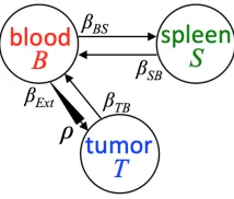
Although different types of CAR T therapy (CAR T therapy alone, CAR T therapy with added CXCR1 chemokine receptors, CAR T therapy with added CXCR2 chemokine receptors, etc.) were studied during these experiments, we only investigate CAR T therapy alone in this manuscript. We do this by modeling the flow of T-cells in the tumorT, T-cell in the bloodB, and T-cell in the spleenS of a single mouse in the system of ordinary differential equations (ODEs),

d~x(t)

dt = d dt





T(t)

B(t)

S(t)



= 



ρβExtB−βT BT

(βT BT−ρβExtB) + (βSBS−βExtB)

βExtB−βSBS



 , ~x0=~x(0) =

  T(0) B(0) S(0)  =   T0 B0 S0   (7)

which is first presented in [18] and depicted in Figure 2. The number of T-cells in the blood,B, extravasate to the tumor,T, at a rateρβExt. For each T-cell that leaves the blood, there may be a transient expansion,

ρ, in the tumor due to antigen recognition. The T-cells in the tumor,T, flow back to the blood,B, at a rate

βT B, T-cells in the blood flow to the spleen, S, at a rateβExt, and T-cells flow from the spleen back to the

blood at a rateβSB. Based on biological assumptions established in [18], we setβExt= 0.01,βT B= 0.001,

βSB = 0.0001, B0 = 106, and T0 = S0 = 0. We assume that each mouse has a different level of antigen

recognition, ρ, so we assume a probability distribution over this parameter, and our goal is to correctly estimate this distribution.

A sample set of data is simulated using (7) and drawing a different value ofρfrom the normal distribution with mean 15 and variance 1 for each mouse in the data set. We choose this mean of 15 due to previous estima-tions regarding the value ofρfor the CAR T therapy [18]. Hence, given that~x(t;ρ) = [T(t;ρ), B(t;ρ), S(t;ρ)] are solutions to (7),

~uij = [Tij, Bij, Sij]T

| {z }

simulated aggregate data

= ~x(tj;ρij) | {z }

model

+

q

~

x(tj;ρij)◦~ij

| {z }

weighted observational error

(8)

represents aggregate data collected from theith _{mouse sampled on the}_jth _{time point. Each}_ρ

(6)

indepen-Figure 2: Schematic of the simple compartmental model described in (7).

N(0,0.10), and◦is the Hammond product, so that the simulated data has weighted observational error [4]. Note that we can average this simulated data in order to obtain exactly one data point~uj = _N1 Pi~uij per

time point.

Rather than use Bayesian analysis to estimate the distribution ofρ, we formulate an aggregate model,

~u(t;p) = [uT(t;p), uB(t;p), uS(t;p)]T = Z 20

10

~

x(t;ρ)p(ρ)dρ, (9) corresponding to the individual model defined in (7) wherepis the probability density function (PDF) ofρ

(7)

4 Results

In the following sections, we compare results for averaged data (which we callreduced data) and non-averaged data (which we call full data). The reduced data set utilizes five simulated solutions, and then averages them to createN = 1 observations per time point,n. The full data utilizes the same five simulated solutions, but does not average them, creating a sample ofN = 5 observations per time point. Each number of time points, n, is generated uniformly in [0,15], and we know the initial conditions for the Tumor, T, Blood,B, and Spleen,S T-cell solutions are [0,106_,_{0], respectively.}

Case 1:

n

= 3

(8)

(9)

Case 2:

n

= 7

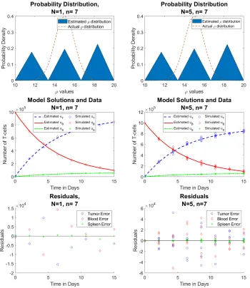
We now have a comparison of reduced and full data, where N is the number of observations per time point, and n = 7 is the number of time points. We see that with both reduced and full data sets, the approximation is not entirely ideal. However, it should be noted that now, both distributions are exactly the same, illustrating that forn= 7, we will have the same results if we average the five mice (givingN = 1 per time point) or if we choose not to average (givingN = 5 per time point).

Figure 4: Reduced data (left) vs. full data (right) forρ∼ N(µ= 15, σ= 1) (Row 1) estimated probability distribution of ρ, (Row 2) n = 7 time points of simulated aggregate data, and (Row 3) residuals | ~u˜j−

~

(10)

Case 3:

n

= 11

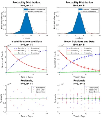
We slightly increase the number of time points to n = 11. Here, we see that the approximations are improving for both the reduced and full data sets, and are identical.

~

(11)

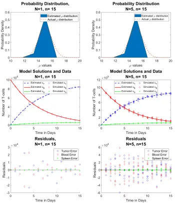
Case 4:

n

= 15

In case 4, we compare the reduced and full data, where N is the number of observations per time point, andn= 15 is the number of time points. The approximations are still improving.

~

(12)

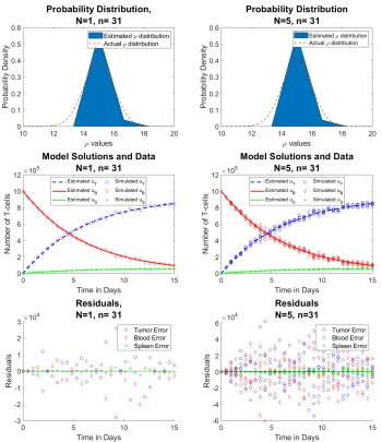
Case 5:

n

= 31

Case 5 shows results for n= 31 time points. Our approximations continue to improve, and there is no difference between the reduced data and the full data.

~

(13)

Case 6:

n

= 39

Lastly, we increase our njust slightly, to n= 39. Here we see the results for the reduced data and the full data. We see that the approximation has actually gotten worse, which could be attributed to too large of ann, and a result of a poor random sample ofρvalues.

~

(14)

5 Practical Identifiability Analysis: Monte Carlo Simulations

Because there are multiple variations of the simulated data, which was simulated through randomly generated ρ values, we now use Monte Carlo simulations to determine the practical identifiability of the probability distribution ofρ. Using techniques from Miao, Xia, Perelson, and Wu [15], we simulateQ= 100 sets of data for each of the 1-6 cases above estimating the probability densities ˆpl(ρ) for each of these l =

1, ..., 100 sets of simulated data, and averaging these estimated densities. We then compare the estimated probability distribution to the actual distribution by comparing the spline nodes to their corresponding place on the actual distribution. That is, with the method of Average Absolute Estimation error (AAE) we estimate the error for each spline node by

AAEk =

1 100

100

X

i=1

|pA(ρk)−pˆl(ρk)| (10)

where ˆpl(ρk) is the kth PDF spline node (k = 1, ..., 5) estimated from the lth Monte Carlo set of simulated

data (l = 1, ..., 100), and pA(ρk) is the actual PDF (the PDF of N(15,1)) at the kth spline node. Note

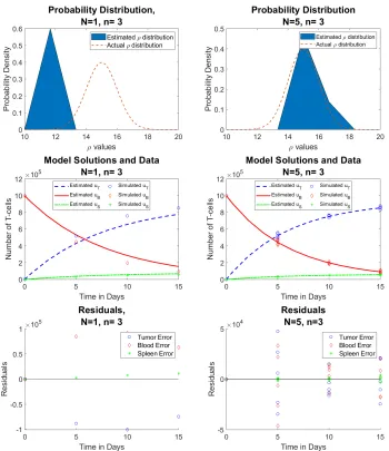
that the full data set (with N = 5 mice per time point) estimates the true PDF significantly better than the reduced data set (where aggregate mice data are averaged at each time point). This is because with the reduced data set the inverse problem is underdetermined, with only n = 3 time points of data (at t = 5, 10, 15 days) and 5 spline nodes of the PDF to be estimated. As shown in the following figures, if we increase the number of simulated time points to ben >5 so that the inverse problem in not underdetermined, the resulting estimated PDF from the full and reduced data set are similar. As shown, the estimated distributions improve as we increase the number of simulated data points, but the distributions are over-dispersed. In other words, this method overestimates the standard error of our parameter of interest,ρ.

Note that this is AAE is different from the average relative estimation error (ARE) as described in [15] which divides the AAE by the true PDFpA(ρ). Since the PDF is very small and close to zero at the tail

ends, the ARE is very large at the tail ends, so we do not calculate the ARE.

(15)

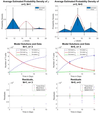
Case 1:

n

= 3

,

Q

= 100

As seen from the figures in the left column, the reduced data sets (N= 1) give, on average, a very poor approximation. Not only does the probability density fail to capture the “actual” distribution, the model solutions do not match the data very well. However, the full data set (on the right) estimates the true PDF significantly better. If we compare this to case 1 from section 4, we will see that here, our average approximated probability density has tails where it did not before. This is due to the nature of the multiple random simulations. Section 4 simply generates one random sample ofρvalues, which may give an inaccurate picture of the entirety of its scope. In the current section, we see the results of many moreρdistributions.

~

(16)

(17)

Case 3:

n

= 11

,

Q

= 100

~

(18)

(19)

Case 5:

n

= 31

,

Q

= 100

~

(20)

(21)

5.1 Comparison of AAE for Cases 1-6: Reduced data and Full data

We now move to the discussion regarding the Monte Carlo simulations, AAE, and average estimated probability density for the previous 6 cases, for reduced data (N = 1) and full data (N = 5). Initially, in Section 4, we only randomly simulated one set of data. By simulatingQ= 100 samples, we can get a more accurate picture of a realistic estimated probability density, as seen in Figures 15 and 16. Figure 15 shows a side-by-side comparison of the average estimated probability densities forρ, computed throughQ= 100 simulations. For the reduced data, we see that the worst approximation occurs whenn= 3, which we know to expect. Approximations improve asnincreases, which we see from Figure 17, which shows how the AAE is largest forn= 3 and then decreases. Now, if we consider the full data, as seen in Figure 16, we see that the average estimated probability density has already started to converge to the “actual” distribution for as low asn= 3. From Figure 17, indeed, we find that the non-averaged data AAE is highest for case 1 and lowest for case 5, when n= 31, and case 6, n = 39. This somewhat contradicts what we found in Figure 8, which shows that the approximation actually gets worse after a certain threshold on n. However, after simulating multiple data sets, and averaging the results of those, it becomes clear that we may not always be able to rely on a single set of random data for accurate information. Furthermore, from Figure 17, we see that the only difference between the AAE for reduced and full data is the case in whichn= 3. The rest of the AAE are the same for values ofn, further solidifying our claim that after a certain value ofn, there is no difference between averaging and not averaging the data. Tables 1 and 3 also give the values for the AAE for each case of data.

We can also quantify these errors through theL2 _{and Infinity Norms, which are shown in Figure 18 and}

in Tables 2 and 4. We continue to see that the lowest errors occur whenn= 31 andn= 39, and the highest errors occur whenn= 3, in both reduced data and full data cases. To find the L2 _{norm, we calculate the}

difference between the average density function, ˆpM _{(as found through averaging the results from the Monte}

Carlo simulations, estimated from the lth set of simulated data for l=1,. . . ,100), and “actual” densitypA at

each of the 7 spline nodes, by measuring the sum of squared differences between the average approximated spline nodes and their corresponding solution on the normal curve. Thus, thisL2 _{norm is defined by}

k∆pk2=

v u u t M X k=0

pA(ρk)−pˆ M₍_ρ

k) 2 (11)

wherepA(ρ) is the true PDF (probability density function) ofPA, and ˆpM(ρ) is the estimated spline

approx-imation of the true PDF, calculated for eachρk nodes, k= 0, ..., M. Similarly, the infinity norm, k∆pk∞,

which takes the maximum vectored error, is defined by

k∆pk∞= max(|∆p0|,|∆p1|, ...,|∆pM|) (12)

(22)

(23)

Figure 17: How AAE varies as time points,n, changes usingReduced(N= 1) and Full(N = 5) data

Figure 18: A comparison of L2 _{norms and Infinity norms}_{as time points change using}_Reduced_data

(24)

Tables

AAE, N=1 (Reduced Data)

n= 3 n= 7 n= 11 n= 15 n= 31 n= 39 [0.0009 0.5503 0.0995 0.3989 0.0995 0.0493 0.0001] [0.0004 0.0595 0.0879 0.1495 0.0891 0.0844 0.0005] [0.0005 0.0530 0.0868 0.1397 0.0878 0.0735 0.0005] [0.0004 0.0622 0.0908 0.1650 0.0879 0.0818 0.0005] [0.0004 0.0376 0.0852 0.1219 0.0936 0.0543 0.0006] [ 0.0005 0.0354 0.0886 0.1318 0.0926 0.0452 0.0005]

Table 1: Values of the AAE at each of the 7 nodes, for M = 0, ...,6 for per number of time points, n, for

Reduceddata

Norms of AAE, N=1

n= 3 n= 7 n= 11 n= 15 n= 31 n= 39

L2 0.6958 0.2206 0.2074 0.2318 0.1877 0.1926

∞ 0.5503 0.1495 0.1397 0.1650 0.1219 0.1318

Table 2: L2 _{and Infinity norms of the AAE for}_Reduced_{data, per}_n_{number of time points}

AAE, N=5

n= 3 n= 7 n= 11 n= 15 n= 31 n= 39 [0.0004 0.0809 0.0945 0.1922 0.0897 0.1064 0.0005] [0.0004 0.0600 0.0891 0.1518 0.0885 0.0851 0.0005] [0.0004 0.0533 0.0857 0.1395 0.0878 0.0732 0.0005] [0.0004 0.0623 0.0897 0.1639 0.0879 0.0803 0.0005] [0.0004 0.0375 0.0852 0.1218 0.0940 0.0545 0.0006] [0.0005 0.0352 0.0881 0.1308 0.0920 0.0452 0.0005]

Table 3: Values of the AAE at each of the 7 nodes, for M = 0, ...,6 for per number of time points, n, for

Fulldata

Norms of AAE, N=5 (Full)

n= 3 n= 7 n= 11 n= 15 n= 31 n= 39

L2 _0.2679 _0.2229 _0.2066 _0.2301 _0.1880 _0.1913

(25)

5.2 The Average Absolute Estimation Error: A Streamlined Case

We know that the number of observations or mice per time point, N, is important when considering the non-average data in the inverse problem. With too few observations, our N is not large enough to produce large-enough degrees of freedom. That is, it is necessary forN≥2. Furthermore, although we can investigate phenomenon for large values ofn, it may not be advantageous to consider such a large sample set of mice, as labs have limited resources. As such, we need to consider more realistic options, for very few mice and very few time points. We will compare calculations forn= 2,3,4,5 time points with N= 2,3,4,5 mice, or observations per time point, noting that we ignore a case in whichn= 2,N = 2, for two mice per two time points, as this would provide too few degrees of freedom.

Figure 19 shows a comparison of the averaged estimated probability density for each combination of

n time points andN observations, for n= 2,3,4,5 and N = 2,3,4,5 and corresponding AAE error bars. We see that, overall, the average probability density tends to improve as bothn andN are increased. The most deviation between the estimated probability density and the actual distribution occurs when n= 2, which is corroborated in Figure 20 and Table 5, node, ˆpM

j (ρi), i = 0, ..., M. in Figure 20 and Table 5,

which shows a comparison of the AAE at each averaged estimated probability density function spline node, ˆ

pl(pk), k=0,. . . ,M for M spline nodes, and l=1,. . . ,100 Monte Carlo simulations. We see that the AAE is

lowest when n = 5, N = 5 and it is highest when n = 2, N = 3 and n = 4, N = 3. This tells us that when considering the fewest possible time points and observations, it would be most advantageous to study 5 observations (or mice) over 5 time points. However, if this is not an option, usingN = 3 mice for either

n = 2 orn = 4 time points will produce a larger AAE. We can further quantify this through theL2 _and

infinity norms.

Figure 21 and Tables 6 and 7 shows the L2 _{and infinity norms for each of the varying}_n_by_N _cases.

We see that L2 _{and infinity norms are lowest for} _n_{= 5,} _N _{= 5 and highest highest for} _n_{= 2,} _N _{= 3 and}

(26)

n=2

n=3

n=4

n=5

N=2 N=3 N=4 N=5

Figure 19: Average Estimated Probability Distribution: A comparison of probability densities asn

(27)

Figure 20: How AAE varies as time points,n, is increased and how number of observations/miceN changes

(28)

Tables

Average Absolute Estimation Error, AAE

N = 2 N= 3 N = 4 N = 5

n= 2 N/A [0.0005 0.1081 0.0927 0.2076 0.0936 0.1560 0.0006]

[0.0005 0.0871 0.0891 0.1744 0.0918 0.1162 0.0005]

[0.0005 0.0981 0.0897 0.1926 0.0905 0.1333 0.0006]

n= 3 [ 0.0004 0.0762 0.0883 0.1745 0.0922 0.1074 0.0004]

[ 0.0004 0.0875 0.0880 0.1973 0.0924 0.1230 0.0005]

[0.0005 0.0978 0.0929 0.1973 0.0891 0.1341 0.0005]

[0.0004 0.0809 0.0945 0.1922 0.0897 0.1064 0.0005]

n= 4 [0.0004 0.0777 0.0901 0.1912 0.0820 0.0963 0.0004]

[0.0004 0.0989 0.0951 0.2080 0.0900 0.1343 0.0005]

[0.0004 0.0792 0.1025 0.1905 0.0890 0.1153 0.0005]

[0.0004 0.0706 0.0836 0.1727 0.0843 0.0883 0.0004]

n= 5 [ 0.0004 0.0922 0.0921 0.1919 0.0901 0.1185 0.0005]

[0.0003 0.0562 0.0895 0.1690 0.0861 0.0793 0.0004]

[0.0005 0.0902 0.0864 0.1892 0.0920 0.1145 0.0005]

[ 0.0004 0.0522 0.0860 0.1552 0.0836 0.0753 0.0005]

Table 5: AAE at each of the 7 nodes, M = 0, ...,6 for varying cases ofN andn

L2 _{Norm of AAE}

N = 2 N = 3 N = 4 N = 5

n= 2 N/A 0.3106 0.2605 0.2841

n= 3 0.2532 0.2793 0.2882 0.2679

n= 4 0.2583 0.2971 0.2725 0.2381

n= 5 0.2756 0.2311 0.2701 0.2165

Table 6: L2_{norm of the AAE for each combination of}_N _and_n

Infinity Norm of AAE

N = 2 N = 3 N = 4 N = 5

n= 2 N/A 0.2076 0.1744 0.1926

n= 3 0.1745 0.1973 0.1973 0.1922

n= 4 0.1912 0.2080 0.1905 0.1727

n= 5 0.1919 0.1690 0.1892 0.1552

(29)

6 Conclusion

When analyzing aggregate data, it is important to treat it as such when performing parameter estimation. Otherwise, even using a powerful uncertainty tool like Bayesian analysis, the uncertainty of an estimated parameters is underestimated. This is demonstrated in Section 2, where aggregate data simulated from a simple logistic model is treated as non-aggregate data.

In Section 3, we simulate data from a more complex biological model and correctly treat this data as aggregate. Instead of using Bayesian analysis, we formulate an aggregate model using techniques from [18] and perform a weighted least squares problem to estimate our parameter of interest. In contrast with Section 2, this method over estimates the standard error of the estimated parameter, and estimates heteroscadicity when there is none. However, it is better to overestimate standard error, and the resulting estimated probability distribution of the parameter is still fairly accurate.

Acknowledgements

This research was supported in part by the Air Force Office of Scientific Research under grant number AFOSR FA9550-18-1-0457.

References

[1] H. T. Banks, A Functional Analysis Framework for Modeling, Estimation and Control in Science and Engineering, CRC Press, 2012.

[2] H.T. Banks, John E. Banks, Natalie G. Cody, Mark S. Hoddle, and Annabel E. Meade, Population model for the decline of HOMALODISCA VITRIPENNIS (HEMIPTERA: CICADELLIDAE) over a ten-year period, CRSC-TR18-06, Center for Research in Scientific Computation, N. C. State University, Raleigh, NC, June, 2018;J. Biological Dynamics,13(2019), 422–446.

[3] H.T. Banks, R. Baraldi, J. Catenacci, and N. Myers, Parameter estimation using unidentified individual data in individual based models, CRSC-TR16-04, Center for Research in Scientific Computation, N. C. State University, Raleigh, NC, June, 2016;Mathematical Modelling of Natural Phenomena, 11, (6) (2016), 103–121. DOI: 10.1051/mmnp/201611607

[4] H. T. Banks, K. Bekele-Maxwell, R. A. Everett, L. Stephenson, S. Shao, and J. Morgenstern. Dynamic modeling of problem drinkers undergoing behavioral treatment, CRSC-TR16-12, N. C. State University, Raleigh, NC, October, 2016. Bulletin of Mathematical Biology,79(6) (2017) 1254–1273.

[5] H.T. Banks and K.L. Bihari, Modeling and estimating uncertainty in parameter estimation, CRSC-TR99-40, December, 1999; Inverse Problems,17(2001), 95–111.

[6] H.T. Banks, D.M. Bortz, G.A. Pinter and L.K. Potter, Modeling and imaging techniques with potential for application in bioterrorism, CRSC-TR03-02, January 2003; Chapter 6 inBioterrorism: Mathematical Modeling Applications in Homeland Security (H.T. Banks and C. Castillo-Chavez, eds.), Frontiers in Applied Math, FR28, SIAM, Philadelphia, 2003, 129–154.

(30)

[8] H. T. Banks, S. Hu and W. C. Thompson,Modeling and Inverse Problems in the Presence of Uncertainty, CRC Press, Boca Raton, FL 2014.

[9] H.T. Banks, Z.R. Kenz and W.C. Thompson, A review of selected techniques in inverse problem nonparametric probability distribution estimation, CRSC-TR12-13, May 2012; J. Inverse and Ill-Posed Problems,20(2012), 429–460

[10] H. T. Banks and W. Clayton Thompson, Random delay differential equations and inverse problems for aggregate data problems, CRSC-TR18-07, Center for Research in Scientific Computa-tion, N. C. State University, Raleigh, NC, July, 2018; Eurasian J. Mathematical and Computer Applications, 6 No. 4 (2018 ), 4–16.

[11] H. T. Banks and Hien T Tran, Mathematical and Experimental Modeling of Physical and Biological Processes, CRC Press, Chapman & Hall, Boca Raton, FL, 2009.

[12] D. Abate-Daga and Marco L Davila, CAR models: next-generation CAR modifications for enhanced T-cell function, Mol Ther Oncolytics May 18; 3(2016) :16014. doi: 10.1038/mto.2016.14. eCollection 2016.

[13] Gerda de Vries, Thomas Hillen, Mark Lewis, Johannes Muller, and Birgitt Schonfisch, A Course in Mathematical Biology: Quantitative Modelling with Mathematical and Computational Methods, SIAM, Philadephia, 2006.

[14] Annabel E. Meade, H.T. Banks, John E. Banks, Natalie G. Cody, and Mark S. Hoddle, Delay differential population models for the decline of HOMALODISCA VITRIPENNIS (HEMIPTERA: CICADELLI-DAE) densities over a ten-year period, CRSC-TR18-08, Center for Research in Scientific Computation, N. C. State University, Raleigh, NC, September, 2018; Proc. 2019 American Control Conference, to appear.

[15] Hongyu Miao, Xiaohua Xia, Alan S. Perelson, and Hulin Wu, On identifiability of nonlinear ODE models and applications in viral dynamics,SIAM Review,53(1) (2004), 3–39.

[16] Edmund K. Moon, Carmine Carpenito, Jing Sun, L.C. Wang, V. Kapoor, J. Predina, D.J. Powell Jr, J.L. Riley, C.H. June, S. M. Albelda, Expression of a functional CCR2 receptor enhances tumor localization and tumor eradication by retargeted human T cells expressing a mesothelin-specific chimeric antibody receptor, Clinical Cancer Research,17(14) (2011), 4719–4730.

[17] S. I. Rubinow, Introduction to Mathematical Biology, John Wiley & Sons, New York, 1975.

[18] Celia Schacht, Annabel Meade, H.T. Banks, Heiko Enderling, and Daniel Abate-Daga, Estimation of probability distributions of parameters using aggregate population data: Analysis of a CAR T-cell cancer model, CRSC-TR19-04, Center for Research in Scientific Computation, N. C. State University, Raleigh, NC, March, 2019;Mathematical Biosciences and Engineering, submitted.