Volume 2010, Article ID 525026,19pages doi:10.1155/2010/525026
Research Article
A Macro-Observation Scheme for Abnormal Event Detection in
Daily-Life Video Sequences
Wei-Yao Chiu and Du-Ming Tsai
Department of Industrial Engineering and Management, Yuan-Ze University, 135 Yuan-Tung Road, Nei-Li, Tao-Yuan 32026, Taiwan
Correspondence should be addressed to Du-Ming Tsai,[email protected]
Received 19 October 2009; Revised 4 March 2010; Accepted 8 April 2010
Academic Editor: Robert W. Ives
Copyright © 2010 W.-Y. Chiu and D.-M. Tsai. This is an open access article distributed under the Creative Commons Attribution License, which permits unrestricted use, distribution, and reproduction in any medium, provided the original work is properly cited.
We propose a macro-observation scheme for abnormal event detection in daily life. The proposed macro-observation representation records the time-space energy of motions of all moving objects in a scene without segmenting individual object parts. The energy history of each pixel in the scene is instantly updated with exponential weights without explicitly specifying the duration of each activity. Since possible activities in daily life are numerous and distinct from each other and not all abnormal events can be foreseen, images from a video sequence that spans sufficient repetition of normal day-to-day activities are first randomly sampled. A constrained clustering model is proposed to partition the sampled images into groups. The new observed event that has distinct distance from any of the cluster centroids is then classified as an anomaly. The proposed method has been evaluated in daily work of a laboratory and BEHAVE benchmark dataset. The experimental results reveal that it can well detect abnormal events such as burglary and fighting as long as they last for a sufficient duration of time. The proposed method can be used as a support system for the scene that requires full time monitoring personnel.
1. Introduction
Activity recognition has played an important role in video surveillance for security, traffic-monitoring, homecare, and healthcare applications. An activity recognition system gen-erally involves the following four steps: low-level detection of moving objects from the background with a still camera, spa-tiotemporal representation of motions in an image sequence, extraction of motion features from the representation, and high-level classification.
There are two major approaches for activity recogni-tion in video sequences: micro-observarecogni-tion and macro-observation. The micro-observation approach analyzes the motions based on the local detailed parts of individual moving objects. In human motion analysis, this means the body parts such as head, torso, and limbs must be identified first, followed by poses assignment based on the extracted body parts. The poses then construct a specific action, and finally a sequence of actions gives a meaningful behavior. This approach requires a bottom-up process to construct a representation from the low-level primitives
of foreground objects. The macro-observation approach does not describe the motion of an object by the local details. Instead, it describes the motion from a global aspect using an abstract representation of time-space changes in a video sequence. Human beings have the remarkable ability to recognize the behavior of a single isolated person, or the interaction between multiple people from a far distance without knowing the detailed motions of individual persons.
In this paper, we propose a fast macro-observation surveillance scheme that can detect abnormality in our daily life that involves distinct activities of a single person or a group of people. A video surveillance system that can monitor abnormal events in daily life is very complicated to construct due to unanticipated or indefinable activities.
objects from the background and precise identification of the individual body parts. An inaccurate extraction and description of details in a lower level causes the failure in a higher level process.
Appearance-based methods [1–6] used appearance mod-els that combine shape, color, and texture to analyze the moving objects. Model-based methods constructed a human body as articulated/kinematic or skeleton models [7–13]. The poses identified from the object models were considered as individual states in space, and then hidden Markov models (HMMs) [14–18] were generally used to describe the state changes over time. Bayesian networks and neural networks [19–21] were also commonly used for high-level activity recognition.W4 [5] is a well-known system using such an
approach to recognize events between people and objects. This approach is also well applied to gesture recognition [22, 23] and gait recognition [24, 25]. Shah et al. [26] presented a surveillance system, called KNIGHT, that used rule-based algorithms to detect single object activities and multiobject interactions. Speed, direction, and orientation of object silhouettes and their interobject distances were used as features to detect activities such as falling, running, and meeting.
1.2. Macro-Observation Approach. Spatiotemporal represen-tation of an image sequence is critical for recognizing diff er-ent activities using the macro-observation approach. Optical flow [27–30] that describes each pixel in two consecutive frames by a velocity vector has been popularly used as a motion representation. Efros et al. [31] recognized human actions of individuals in a low resolution video sequence. Their algorithm started by tracking individual human figures and forming a figure-centric sequence. Then the optical flow vector field was calculated from the figure-centric sequence, and a set of motion descriptors were derived from 4 channels of the optical flow. The K-nearest neighbor classifier was finally used to recognize various human actions in sport videos.
Trajectory [32–36] is a commonly-used representation for describing moving objects from a far distance. In order to construct the trajectory of moving objects in an image sequence, object tracking is generally applied first, and then the centroid of a tracked object is marked as a point on the trajectory. The position, speed, direction, and curve/shape of the motion trajectory are used to analyze the intended behaviors of moving objects in the scene. The trajectory representation has been mostly applied to traffic monitoring. Stauffer and Grimson [37] used vector quantization to cluster trajectories for parking lot monitoring. The clusters were identified by a hierarchical analysis of the vector cooccurrences in the trajectories. The trajectory is good for the representation of a widely open scene, but may fail to describe the people interaction in a room-sized scene.
Eigenspace [38–41] derived from principal component analysis is also used for motion representation in video sequences. Rahman and Ishikawa [42] recognized human motion using an eigenspace. A 2D spatial image was first arranged as a column vector. Then, a series of a fixed number of consecutive images for every possible motion to
be recognized were organized as a matrix. The eigenvectors with dominant eigenvalues of the covariance matrix formed the eigenspace. A human posture in a frame was then represented by a point in the eigenspace, and a motion was described by a set of successive points in the eigenspace. Distance measures were finally used to match the lines of the observed motions and those of the reference motions. The eigenspace approach is computationally expensive and can only describe specific activities.
Motion Energy Image (MEI) and Motion History Image (MHI), first proposed by Davis and Bobick [43], are a global spatiotemporal representation of motion. They are treated as temporal templates for the match of human movement [44]. MEI is defined as the sum of object silhouettes in every image frame over a fixed duration. The result of MEI is a binary image of motion shape. While MEI is used to record the “shape” of a motion, the intensity of MHI is a function of recency of motion. The effectiveness of the MEI and MHI representations is critically determined by the fixed duration value. Bradski and Davis [45] extended the MHI for motion segmentation and pose recognition by extracting additional pose and directional motion information in MHI. The gradient orientation at each pixel is derived from the spatial derivatives along the y- and x-axis of MHI. Wong and Cipolla [46] also used the gradient directions in MHI for gesture recognition. Davis and Bobick [47] used MHI for recognizing aerobic movements. The temporal templates of MEI and MHI were also used for hand gesture recognition [48]. The temporal template has shown to be a good global representation of motions. However, it is currently only verified for simple activities such as hand gestures and aerobic exercises that have a fairly steady motion duration and is only tested for single isolated object in a simple background.
used as the features. A fuzzy self-organizing neural network was then presented to classify the activity patterns. The system was applied in traffic monitoring to detect abnormal driving trajectories.
Fleet et al. [51] and Andrade et al. [52] used optical flow patterns to detect emergency events in crowded scenes. They first computed the optical flow for the whole frame, and retained only the flow information in the foreground region. Principal component analysis was then performed on the optical flow fields for a series of image frames of fixed duration. The dominant eigenvectors of the training data matrix were used to form bases for the projection. The projected optical flow vectors were then used as features. A mixture of Gaussian hidden Markov model was trained with the feature vectors for each video segment in the training set, and the spectral clustering was used to determine the number of HMMs to represent various flow sequences. For day-to-day behavior analysis, an extremely large set of training image sequences may be required. The covariance matrix of such a large training set could be prohibitively large for PCA computation. Adam et al. [53] proposed an optical flow-based method for unusual event detection in cluttered and crowded environments. The abnormality was mainly detected by evaluating the probability distribution of flow magnitude and direction in the optical flow fields. An unusual event without radical motion changes cannot be detected with this method.
Zhong et al. [54] presented a technique for detecting unusual activities in video sequences. Moving objects in each image frame were detected first. The simple spatial histogram of the detected objects was used as image features and, therefore, the observed activities were location-dependent. They divided the video into equal-length segments and classified the extracted features into prototypes. A cooccur-rence matrix between the video segments and prototype features was constructed for similarity comparison. The correspondence between prototypes and video segments was then solved as a graph editing problem.
The abnormal event detection methods aforementioned generally consider the motions of objects with a fixed observation duration (i.e., a predetermined number of image frames) in video sequences, and require well-controlled environments or well-defined patterns of activities. Most of the currently available activity recognition methods only deal with very simple activities, and are domain specific such as aerobic exercises [44] and tennis strokes [55]. In this study, we propose a macro-observation approach to detect abnormal events observed, especially, in a room-sized scene from a still camera. The scene of a room may involve complicated day-to-day behaviors such as an older person staying alone at home (for homecare monitoring), multiple people with/without interaction in a nursing home (for healthcare monitoring), and cashier-customer interaction in a shop (for security monitoring). The observed objects in such scenes have moderate sizes in the image. The trajectory representation of an object as a point may lose meaningful interaction between people. The proposed method does not take the micro-observation approach since it requires complicated object tracking, object segmentation and body
part extraction, and state-space modeling for all possible events to detect. The abnormal events in a daily life are very difficult to define semantically, and the normal events are too numerous to model individual day-to-day activities.
1.4. Overview of the Proposed Method. With the macro-observation approach, the proposed method first segments moving objects from the background for each input scene image. The foreground objects shifting in spatial images over time are globally represented by an energy map, where the movement strength of each pixel in the current scene image is exponentially increased/decreased based on the state changes of the pixel over time. The length of image frames for different activities does not have to be explicitly specified, and the energy map can be promptly updated for each new scene image. The shape of the energy map and movement strength of every pixel in the map carry meaningful time-space interaction of single person or multiple people with the environment. A set of discriminative features can then be effectively extracted from the energy map of each new scene image.
Abnormal event detection in daily life can be considered as a very special case of one-class classification problem. No all possible abnormal event in daily life can be foreseen. It is also very difficult to collect all possible conditions of a specific abnormal event. Conversely, normal behaviors in daily life can be easily collected for learning. The behaviors repeated daily can be grouped into many clusters, and all clusters belong to the same class, that is, the normality class. Because the types of normal behaviors in a daily life could be numerously large and quite different from each other, the images are randomly sampled from a long image sequence that can sufficiently represent the cyclical day-to-day activities of the observed scene. An unsupervised clustering subject to distance constraints is proposed to group various normal activities into a manageable number of clusters so that the computation in the recognition process can be efficiently carried out and all normal events can have distances from their cluster centroids within very tight control limits (distance thresholds). The video images with distinct feature distances lasting for an extended period of time are then declared as an abnormal event.
The proposed macro-observation method mimics the human observer who can easily recognize abnormal events from a far distance without knowing the detailed move-ments of individual persons. The global representation of complicated motions in a scene can well detect abnormal events as long as they can last for tens of seconds. Since the detailed motions of individual body parts are not separately extracted, the proposed method cannot be responsive to the events with subtle motion changes and the events spanning only a few seconds. The proposed monitoring system can be used as a supplement for the personnel that requires intensive and constant manual monitoring of scenes for unpredictable events from multiple cameras.
followed by the extraction of discriminative features from the energy map. The proposed clustering mechanism is then presented to group similar energy maps sampled from image sequences of normal daily life.Section 3describes the experimental results of daily activities in a laboratory over a long period of observation and the BEHAVE benchmark dataset [56]. Section 4 concludes the paper and discusses future work.
2. Abnormal Event Detection
This section discusses the abnormal event detection scheme that comprises the processes of moving object detection, exponential energy map for spatiotemporal representation of motions, extraction of motion features, and the constrained clustering model for classification.
2.1. Moving Object Detection. The objective of the paper is to detect abnormal events in daily life in a scene such as an office or a nursing home, where nonstationary background changes such as movements of a chair, placing of cups and newspapers on tables, revolving of ceiling fans, opening/closing of doors or curtains, and switching on/off room lights are not uncommon. Since the proposed method does not rely on the accurate detail parts of moving objects for the detection, any background subtraction techniques such as the ones in [3,57–59] can be directly applied to foreground segmentation as long as it is computationally fast.
In background updating models, each pixel of the background image over time has been simply modeled with a single Gaussian model [3]. A more robust background modeling technique is to represent each pixel by a mixture of Gaussians [37,57]. In order to promptly detect moving objects for nonstop monitoring of day-to-day activities, we adopt a single-Gaussian background updating approach, instead of the more complicated mixture Gaussian model, to extract foreground objects with a high processing rate.
In the single Gaussian model for each individual pixel in the image, the parameters are represented by the gray-level mean μT(x,y) and standard deviation σT(x,y) of the pixel (x,y) over a limited time duration. Different from the Gaussian background updating models [3,57] that estimate the parameter values by a linear filtering technique, these two statistical values of the single Gaussian model can be easily and precisely calculated by deleting the last image in the series of the historical image frames and adding the current image frame for nonstop monitoring.
Let{ft(x,y), t = T,T−1,. . .,T −N+ 1} be a series ofNconsecutive image frames, whereTdenotes the current time frame. The gray-level mean and variance of the single Gaussian background model for pixel (x,y) at time frameT is given by
μTx,y=Efx,y= 1
NST
x,y,
σT2
x,y=Ef2x,y−Efx,y2
= 1
N ·S
2
T
x,y−μ2
T
x,y,
(1)
where
STx,y=
N−1
i=0
fT−i
x,y
=ST−1
x,y−fT−N
x,y+fTx,y,
S2
T
x,y=
N−1
i=0
f2
T−i
x,y
=S2T−1
x,y−fT2−N
x,y+fT2
x,y.
(2)
Note thatST(x,y) andS2T(x,y) can be efficiently updated by dropping the last image frame fT−N(x,y) in the image series and adding the current image frame fT(x,y) to the image series. Therefore, the updating computation involves only two simple arithmetic operations. A very high process rate of image frames is achieved accordingly. Note also that the mean and variance updating processes in (1) are invariant to the number of image framesNin the series.
In motion detection, the multiple temporal images of the background will present approximately the same gray value with a small variance. The gray value of a foreground pixel will be distinctly different from that of the background. The upper and lower control limits for foreground-pixel detection in the current image frame fT(x,y) can be given byμT−1(x,y)±κ·σT−1(x,y), whereκis a control constant.
If the gray-level of fT(x,y) is out of the control limits, pixel at (x,y) is then considered as a foreground point. Otherwise, it is classified as a steady background point. The detection result is represented by a binary imageBT(x,y), where
BTx,y=
⎧ ⎪ ⎪ ⎪ ⎪ ⎨ ⎪ ⎪ ⎪ ⎪ ⎩
0background, iffTx,y−μT−1
x,y
≤κ·σT−1
x,y,
1foreground, otherwise.
(3)
Since the gray values between foreground and background points are generally distinctly different, the control constant κis set at 5 in this study.
2.2. Spatiotemporal Representation. The goal of this sub-section is to construct a global representation of motion that can describe the changes in both temporal and spatial dimensions. The existing spatiotemporal representations of motions aforementioned generally describe the temporal context with a fixed duration in a video sequence. The motion representation from a fixed number of image frames may not sufficiently capture the salient and discriminative properties for a large variety of activities encountered in daily life. Short observation duration cannot describe a full cycle of an activity. In contrast, excessively long observation duration may mix two or more different activities or reduce the significance of a unique activity in the spatiotemporal representation.
of activities, we construct the motion energy map using an exponential time update process, which is defined as
ETx,y=MT+ET−1
x,y·γ, (4)
whereγis the energy update rate, 0< γ <1, and
MTx,y=
⎧ ⎨ ⎩
Tenergy, ifBT
x,y∈foreground,
0, otherwise. (5)
The initial value of energy is set to zero at time frame 0, that is, E0(x,y) = 0 for all pixels. The energy of a pixel
ET(x,y) will be increased if it remains as a foreground point. It is only decayed when it becomes a background point. In (4) above,Tenergyis a predetermined energy constant, and is
assigned to each foreground pixel. Assume that the current energy value of a pixel (x,y) isE. If pixel (x,y) is a foreground point and lasts for a period ofNf frames, then the energy at (x,y) is increased up to
Tenergy·
Nf−1
i=0
γi+E·γNf. (6)
Conversely, if pixel (x,y) is changed from a foreground point to a background point and lasts forNbframes, the energy at (x,y) is then exponentially decreased to
E·γNb. (7)
The choice ofTenergyvalue is not critical at all as long as
it is larger than zero for foreground points and equal to zero for background points. The value ofTenergyaffects only the
visual representation of the energy map in the image. It does not change the detection results.
The exponential energy updating of foreground pixels assigns larger weights to the most recent image frames. The energy update rateγgives an exponential decrement of the energy. A largeγvalue gives a slow decrement of the energy, and the long-term history of the pixel is taken into account for spatiotemporal representation. In contrast, a small γ value results in an accelerated decrement of energy, and only the short-term history of the pixel is used to represent the motion. The exponential decrement of energy allows flexible adjustment of the observed period for the historical status of each pixel. The proposed exponential energy map of motions prevents the explicit choice of a predetermined number of image frames for the construction of spatiotemporal representation. It can be thus effectively used to represent activities that last for various durations. By detecting each individual pixel as a foreground or a background point in the video sequence, the energy of the pixel can be easily updated according to (4) without knowing its associated moving part of an object. If the motion of the pixel continues (i.e., foreground point), the energy of the pixel will be exponentially accumulated. Otherwise, the energy of the pixel (i.e., background point) will be decreased. In the macro-observation approach, two (or multiple) movements within a scene is simply interpreted as an event in the energy
map. They do not have to be separated into different moving parts.
Figure 1 displays the motion energy maps of various video sequences of one single person from daily activities in a laboratory, in which the energy constantTenergy is set
at 10 for visual display, and the update rate γ is given by 0.999 for the normal walking speed of people in the room. The video images were taken at 10 frames per second. Figure 1(a) shows the original video sequence at varying time frames. The scenario in the sequence is that a single person walked towards the door from the lower-left to the upper-right in the scene. The resulting energy map is shown in the bottom row of Figure 1, where the brightness is proportional to the energy value. Figure 1(b) presents another single person walked from the upper-right door to the lower-left corner in the opposite direction. By closely observing the two corresponding energy maps in Figures 1(a)and1(b), both display similar representations in shape. The energy values in the upper-right are higher than those in the lower-left in the energy map ofFigure 1(a), whereas the energy values in Figure 1(b)show the reverse trend. Therefore, the representative shape of the energy map describes various spatiotemporal activities, and the changes of energy values in the map implicitly indicate the moving direction. Figure 1(c) displays a single person working on a computer. The resulting energy map, as seen in the bottom row ofFigure 1(c), shows that only the sitting area of the person gives bright energy values. The historical data of the movement from the lower-left to the upper-right corners were responsively decayed to very small energy values.
Figure 2(a) shows a group of people discussing in the middle-right area for a prolonged period of time, and then walked back to their seats. The bottom row in Figure 2(a) gives the corresponding energy map, in which the middle-right area is bmiddle-righter than the remaining regions in the image and the energy values for pixels in the walking paths are larger than those of the background.Figure 2(b)shows two people chatting around the public desk in the laboratory, and Figure 2(c) displays two people separately working on the computers. The corresponding energy maps are presented in the bottom row of Figures 2(b) and 2(c), which show that different moving frequencies of multiple people generate different energy maps. Based on the representative samples in Figures1and2, the exponential energy maps can represent different day-to-day activities that involve single or multiple people.
t=1
t=10
t=15
t=20
(a)
t=1
t=10
t=15
t=20
(b)
t=1
t=10
t=15
t=20
(c)
Figure1: Video sequences involving different activities of a single person and their corresponding energy maps: (a) single person walking from lower-left to upper-right; (b) single person walking from upper-right to lower-left; (c) single person working on a computer. The corresponding energy map of each column sequence is shown in the bottom row.
2.3. Discriminative Features. The proposed exponential energy map gives spatiotemporal representation of an activ-ity. To construct a classification system for identifying abnor-mal events, we need to design and extract discriminative
t=1
t=100
t=200
t=300
(a)
t=1
t=100
t=200
t=300
(b)
t=1
t=100
t=200
t=300
(c)
Figure2: Video sequences involving different activities of multiple people and their corresponding energy maps: (a) a group of people discussing in the middle-right area; (b) multiple people chatting around the public desk; (c) multiple people working on the computers. The corresponding energy map of each column sequence is shown in the bottom row.
Invariant Moments f1 to f7. an event in the energy map forms a specific shape with the energy magnitude of each pixel as the weight. The extracted features from the energy map should be independent of location, orientation and size
of an activity in the image. The first seven discriminative features are, therefore, based on Hu’s invariant moments [60]. Features f1 ∼ f7 are invariant to position, rotation
study are not merely computed from the binary shape, but use the energy valueET(x,y) as the density for each pixel in the energy map.
Entropy f8. letET(x,y) be the normalized energy value into integer in the range between 0 and 255 (for an 8-bit display). Thus
ET
x,y=
ETx,y−Minu,vET(u,v)
Maxu,vET(u,v)−Minu,vET(u,v)×
255
.
(8)
Denote by Pi the probability that ET(x,y) = i,i = 0, 1, 2,. . ., 255. The entropy of the energy map is therefore defined as
f8= −
i
Pi·logPi. (9)
The entropy feature describes the complexity of move-ments in a scene. A still scene will have an entropy value approximate to zero. A single person sitting in a chair for study will yield a small entropy value, whereas a scene involving interaction and movements of multiple people will result in a large entropy value.
Maximum Energy f9. the maximum energy is defined as f9=Max
x,y ET
x,y. (10)
This feature gives the maximum energy value in the energy map. A foreground object that keeps moving for a prolonged period of time will have a larger feature value of
f9, compared to that for a short period of time.
Total Energy f10. the total energy is defined as f10=
x
y
ETx,y. (11)
A scene with a group of people generally yields a larger total energy value, compared to the scene with a single person. A person who keeps moving around in the scene will generate a larger total energy value, whereas a person sitting for study will result in a smaller total energy value.
Area of Nonzero Energy f11. this feature is defined as f11=
x
y
bx,y, (12)
where
bx,y=
⎧ ⎨ ⎩
1, ifETx,y>0
0, otherwise. (13)
A wide moving area will result in a larger feature value of f11, even if the movement lasts for only a very short period
of time, whereas a limited moving area will have a smaller feature value even if the movement lasts for a prolonged period of time.
Mean Energy f12. the mean energy is defined as
f12=
x
yET
x,y
x
yb
x,y = f10
f11. (14)
This feature gives the mean energy value in the region of nonzero energy. The total energy f10for highly repetitive
activities in a small limited area may be similar to that for nonrepetitive activities in a wide area. The mean energy can be used to describe the relationship between the repetitive motions and the moving area.
As demonstration examples, Figures3(a1)–3(a3) present the energy maps of people sitting in chairs for study, Figures 3(b1)–3(b3) display the energy maps of a single person walking in different directions, and Figures 3(c1)–3(c3) are the energy maps of the interaction between multiple people. The corresponding features values of f1 ∼ f12 for
the individual energy maps are summarized in Table 1. It shows that similar activities yield similar feature values, and different activities result in distinct feature values.
2.4. Classification. The discriminative features extracted from the motion energy maps can now be used to identify abnormal events from the normal activities in daily life. Monitoring of abnormality in daily life is not possible to be restricted only to the recognition of prestudied and premodeled events. As aforementioned, there could have numerous distinct daily-life activities in an observed scene. It is extremely difficult to apply a supervised classification system, where each input sample must be manually assigned a class index. The selected classification system should be computationally efficient in the detection stage so that it can be easily implemented for on-line, real-time monitoring. The fuzzyC-means (FCM) clustering [61] has been a widely used technique for unsupervised classification. However, the conventional clustering technique only partitions samples into clusters such that the weighted mean distance of each sample to its centroid is minimized. There is no control of the distance variance in each cluster. It cannot handle clusters of different sizes and densities. It is extremely difficult to find a fixed global distance threshold for each cluster to separate normal and abnormal events in video images.
In this paper, a constrained clustering method is applied for training with the objective that the distance of every cluster member to its own cluster center meets adaptively a distance constraint. In order to collect sufficient represen-tative samples of daily life under observation, the training energy maps and, thus, their corresponding discriminative features are randomly sampled from a video image sequence that spans the sufficient period for all possible day-to-day activities. Note that each single input scene image fT(x,y) has its own corresponding energy map ET(x,y). Each training sample in this study means the feature vector (f1,f2,. . .,f12) of an energy map. Based on our
Table1: Feature values for the demonstrative energy maps inFigure 3.
Features Energy maps inFigure 3
3(a1) 3(a2) 3(a3) 3(b1) 3(b2) 3(b3) 3(c1) 3(c2) 3(c3)
f1 1.381 1.636 1.466 2.111 2.108 2.136 2.354 2.496 2.476
f2 2.951 3.627 3.260 4.401 4.577 4.553 5.309 5.507 5.588
f3 4.678 4.630 4.798 7.227 8.090 8.711 7.555 8.126 8.534
f4 4.922 4.647 4.840 7.081 7.111 8.315 8.738 9.571 9.499
f5 9.752 9.286 9.700 14.238 14.871 16.981 16.993 20.433 20.102
f6 6.402 6.461 6.471 9.285 9.412 10.595 11.454 13.215 12.294
f7 10.175 10.829 10.041 15.189 14.854 16.978 17.089 18.421 18.517
f8 0.717 0.708 0.740 1.085 1.309 1.421 1.603 1.747 1.755
f9 186 256 340 253 249 313 361 325 640
f10 103727 106136 161232 381675 435401 513579 860751 1335763 1281152
f11 13084 13248 14248 13231 17102 20284 20063 20177 21571
f12 7 8 11 28 25 25 42 66 59
(a1)
(b1)
(c1) (a)
(a2)
(b2)
(c2)
(a3)
(b3)
(c3)
Figure3: Demonstration examples of energy maps: (a1)–(a3) people sitting in chairs; (b1)–(b3) single person walking in different directions; (c1)–(c3) interaction between multiple people.
2.4.1. Learning Process. In this paper, we are only interested in the classes of normal and abnormal events. Since the abnormal events are unpredictable beforehand, all training samples are normal activities collected from a video sequence of daily life. They all belong to the same class, that is,
classification with distinct patterns problem is to assign similar training samples to the same cluster so that the distance of every member in the cluster to the cluster center meets a minimum distance threshold.
LetX = {x1,x2,. . .,xK}be a set ofKtraining samples,
andvithe centroid of clusteri. The distance between sample xk and the centroidviis denoted byd(xk,vi) = xk−vi2.
The objective of the proposed clustering is given by
Minβ
s.t. d(xk,vi)≤μdi+β·σdi,
if xk∈vi, ∀k=1, 2,. . .,K,
(15)
where μdi andσdi are the mean and standard deviation of
the distancesd(xk,vi) for all members in clusteri, andβis a control constant. The upper control limit μdi +β·σdi is
used as an adaptive distance thresholdTdifor each individual
cluster i. Each member in its own cluster must meet the distance constraint, and the control limit should be as tight as possible.
In this aper, we use a hierarchical clustering technique to group similar energy maps into clusters. In each hierarchical level of the clustering, a small number of clustersCis given, and then the standard fuzzy C-means clustering process is carried out. In the resulting clusters, the Euclidean distance between each assigned member of the cluster and the cluster centroid is calculated so that the mean μdi and standard
deviation σdi for each cluster i can be determined. If the
distance is less than the distance thresholdTdi, the sample
member is retained in the cluster. Otherwise, it is removed from the cluster. This procedure is repeated for every cluster. At the end of the process, all removed samples are considered as a new set of training data, and the fuzzy C-means clustering with C as the number of clusters is performed in the next hierarchical level. The clustering process is expanded to the lower hierarchical levels until the distance of every member in individual clusters is less than its distance thresholdTdi, or the maximum total number of clustersCmax
is met.
At the end of the hierarchical clustering process, the control constant β will be reduced to tighten the distance thresholds if the distance constraints for all training samples under a given total number of clusters Cmax are satisfied.
Otherwise, it is increased to loosen the distance thresholds. The hierarchical clustering process is then repeated with the new control constant. The minimum value of the feasible control constant β can be efficiently obtained by a binary search. The total number of clustersCmax is predetermined,
which is related to the complexity of daily activities in question. Experiments on various scene scenarios have shown that the total number of clusters around 50 and 60 is sufficient to represent different patterns of normal activities in daily life. The number of clusters C in each hierarchical clustering level is given by 10 in this study. The detailed algorithm of the constrained clustering model with minimum adaptive distance thresholds is presented as follows.
Input. The number of clusters C in each level, maximum number of clusters Cmax, and training data set X =
{x1,x2,. . .,xK}.
Step 1. Normalize the feature values.
Letxk=(fk,1,fk,2,. . .,fk,12) be the feature vector, andfk,j be the jth feature of samplek, fork=1, 2,. . .,K
fk,j=
fk,j−μj
σj , j=1, 2,. . ., 12, (16)
where μj andσj are the mean and standard deviation of featurejfor all training samples.
Letxk=(fk,1,fk,2,. . .,fk,12).
Step 2. Perform the standard fuzzyC-means clustering. Letvibe the centroid of clusteri,i=1, 2,. . .,C, and
vi=
K
k=1w
p ik·xk
K
k=1w
p ik,
(17)
wherewikis the weight for training samplekin clusteri,pis weighting exponent (p=2 in this study).
In each iteration,wikis updated by
wik= 1
C j=1
dxk,vi/dxk,vj1/ p−1
, (18)
whered(xk,vi)= xk−vi2
. Then the centroidviis updated using the new assigned weightwik. The updating procedure is repeated until convergence.
LetVr = {vr
i}Ci=1be the resulting set of cluster centroids
at hierarchical levelr(Initially, setr=1).
Step 3. (a) Assign sample xk to cluster vri, for k = 1, 2,. . .,K, wherei=arg mincd(xk,vr
c).
(b) Set the distance threshold of each cluster vri, i = 1, 2,. . .,C, to
Tdi=μdi+β·σdi, (19)
where μdi and σdi are the distance mean and standard
deviation of clusteri.
(c) LetXri =φandXir=φ, fori=1, 2,. . .,C. Given that xk∈vir,k=1, 2,. . .,K, ifd(xk,vir)< Tdi, then assign
Xri ←−Xri
xk, (20)
otherwise,
Xri ←−Xri
xk. (21)
At the end of the assignment,Xircontains all the members that meet the distance constraints, that is,d(xk,vri)< Tdi, in
clusteri. The centroid of clustervri is updated by
vri = 1 Xri
xk∈Xri
xk, (22)
Xri records the samples withd(xk,vri) > Tdi. LetXr =
C
i=1Xri, which is the set that contains all the samples that violate the distance constraints at iteration r. It is passed along to the next hierarchical levelr+ 1 as a new training set.
Step 4. Cluster in the lower hierarchical level.
TakeXras the set of new training data. Letr←r+ 1. Repeat Steps2and3untilr·C > Cmax(max. number of
clusters is violated), orXr=φ(all samples meet the distance constraints).
Step 5. Find the minimum control constantβ.
Ifr·C > CmaxandXr=/ φ, the current control constantβ
is too tight, and must be increased by setting
β←− 1
2
β+βupper
, (23)
else setting
β←− 1
2
β+βlower
. (24)
Repeat Steps 2 to 5 unit Δβ < 0.1, where Δβ is the difference between the old and the newβvalues. Currently, the lower bound and upper bound ofβare set atβlower=0.0
andβupper=2.0.
The proposed clustering model can effectively assign similar activities into the same cluster that all adaptively meet a tight distance threshold. It is expected that normal activities similar to the sampling ones in the training set will also have a corresponding cluster that meets the distance threshold, whereas an abnormal event (the one not observed in the training set) will not find any cluster that yields a distance less than the threshold.
2.4.2. Detection Process. Let Ω = rVr be the set of the final cluster centroids obtained from the training process. For a new scene image at current time frame T with the feature vectorxT = (fx,1,fx,2,. . .,fx,12), the feature value is
first normalized with respect to the meanμj and standard deviationσjfor each featurejof the training samples, that is,
fx,j=
fx,j−μj
σj , j=1, 2,. . ., 12, (25)
and letxT =(fx,1,fx,2,. . .,fx,12). The minimum distance of
xT to the cluster centroids inΩis given by
dxT,vi∗=min
vi∈Ω
xT−vi2, (26)
wherevi∗ =arg minvi∈Ωd(xT,vi).
In the training process, the distance threshold Tdi of
each cluster i is adaptively given by μdi + β·σdi. In the
detection process, the same distance threshold of each cluster is also applied to detect abnormal events. If d(xT,vi∗) > Tdi∗, a suspected abnormal event is declared. Otherwise,
it is classified as a normal activity in daily life. Since an
abnormal event will generally last for an extended period of time, a single alarm of xT is treated as noise. When the motion energy maps haved(xT,vi∗)> Tdi∗and prolong for a
sufficient duration, an abnormal event is evidently detected. Since the detection process involves only simple Euclidean distance computation from a small set of cluster centroids, it is computationally very fast.
3. Experimental Results
This section evaluates the performance of the proposed abnormality detection scheme from two image sequences, one involving the scene of a laboratory and the other obtained from the BEHAVE benchmark dataset. The pro-posed algorithms were implemented using the C++ language on a Pentium 4, 3.0 GHz personal computer. The test images in the experiments were 200×150 pixels wide with 8-bit gray levels. The total computation time from foreground segmentation to abnormality detection for an input image is 0.132 seconds, of which the computation of the seven invariant-moments takes 0.121 seconds. It achieves a mean of 7.6 fps for real-time detection of abnormal events.
The first activity monitoring example is the daily work in a laboratory, which involves various activities of a single person and multiple people. Some of the demonstration activities in the laboratory are displayed in Figures1and2. The training image sequences were collected for two days, and there are a total of 100,216 energy maps. 15% of the total energy maps were randomly sampled, which corresponds to 15,030 energy maps used in training. In the experiments, the two parameters used to construct the motion energy maps were set withTenergy = 10 andγ = 0.999 for the relatively
slow activities in the laboratory. The total number of clusters Cmaxis given by 50. The resulting minimum feasible value of
the control constantβis 0.1.
In the experiments, we simulated three abnormal events including burglary, fighting and moving furniture out of the room. All these three activities are very difficult to define explicitly and model beforehand. Scenario 1 involves only the actions of a single person. Scenarios 2 and 3 involve interactions between two people. For the burglary scenario, a person was asked to find a wallet hidden in the room as fast as possible. No further instructions on how to find the wallet were given to the pretended burglar. Figure 4(a) displays the original video sequence at varying time frames for the burglary scenario, andFigure 4(b)shows the corresponding energy maps. It can be seen that the energy in the map is weak in the early stage of the burglary activity. The energy is then accumulated and the shape in the map becomes stable after a sufficient period of time.
t=80
t=240
t=480
t=720
t=960
t=1250
(a) (b)
Figure4: Abnormal event of a burglary scenario: (a) discrete image frames in the sequence; (b) corresponding energy maps. (symbolt
represents the frame number in the sequence with fps=10).
scenario. The energy is accumulated and the shape becomes clear in the map as the activity proceeds.
When the training is done, 85% of the untrained image frames (a total of 85,186 frames) from the two-day video sequence are used to test for the similarity measurement.
t=60
t=160
t=320
t=500
t=780
t=900
(a) (b)
Figure5: Abnormal event of a fighting scenario: (a) discrete image frames in the sequence; (b) corresponding energy maps.
t=70
t=210
t=420
t=620
t=830
t=1030
(a) (b)
Figure 6: Abnormal event of a moving-furniture scenario: (a) discrete image frames in the sequence; (b) corresponding energy maps.
Tdi∗, the plot inFigure 7displays only the difference between
the distance d(xT,vi∗) and the threshold Tdi∗, that is,
Δd(xT,vi∗)=max{d(xT,vi∗)−Tdi∗, 0}. In the figure, thex -axis presents the event number and they-axis is the excessive
1 3 5 7 9 11 13 15 17 19 21 23 25 27 Event number
0 2 4 6 8 10
Δ
d
Figure 7: Excessive distancesΔd over the thresholdTΔd for the
27 detected events with distances beyond the control limits in the normal 2-day laboratory video sequence. (The length of each event in thex-axis represents the event duration.)
Burglary Fighting Moving furniture
0 2 4 6 8 10
Δ
d
Figure8: Excessive distancesΔdof the three abnormal events in the laboratory: burglary, fighting and moving furniture out of the room. (Note that the duration scales in thex-axis of both Figures7
and8are the same.)
distanceΔd. The results show that most of the 85,186 frames have the distances within the control limits. All the falsely detected events last only a very few frames (as seen in the x-axis) and the excessive distanceΔdis very small and less than 2 (as seen in they-axis). The duration for the 27 falsely-detected events is from a minimum of 0.2 seconds (1 frame) to a maximum of 4 seconds (20 frames) with a mean of 0.72 seconds (3.6 frames). Because an activity must last for some duration (i.e., a sufficient number of consecutive image frames), the isolated image frames can be classified as noise.
Figures 8 illustrates the measured distances over time for the three abnormal events of burglary, fighting and moving furniture. The plot only displays the distance differences Δd(xT,vi∗). The scale on the x-axis in Figure 8 is exactly the same as that inFigure 7, that is, the length of an event in the x-axis of the figure represents also the duration of the activity. The results show that the abnormal activity at the beginning gives small distance values. As the abnormal activity continues, the resulting distances become distinctly large and prolong for a long duration, as seen in thex-axis and they-axis inFigure 8.Table 2summarizes the resulting statistics of duration and excessive distanceΔdfor the 2-day normal image sequence and the three abnormal events. It again reveals that the proposed detection scheme can well identify the prolonged abnormal activities with distinctly large distances Δd. The falsely-alarmed events give only a very short duration with very small excessive distances and therefore, can be effectively eliminated by introducing additional decision rules based on the event duration.
Table2: Statistical analysis for the two-day normal video sequence of the laboratory scene and the three abnormal events.
Image sequence Total events detected Excessive distanceΔd Alarm duration (sec.)
Mean Std. Min. Max. Aveage
Normal image sequences for 2
days (85,186 frames) 27 0.33 0.39 0.2 4 0.72
Abnormal image sequence 3 3.75 2.18 71.4 182 96
Fuzzy C-means The proposed method 0
2 4 6 8 10 12 14 16
σd
∗
∗
∗ ∗ ∗
Figure9: Box-plots ofσdfor the 50 clusters from the constrained
clustering model and the conventional FCM.
abnormal event detection in this long-observation sequence. The performance of the proposed method on the 31-day image sequence is measured by the false positive rate (false alarms of normal events) given that all the three abnormal events (burglary, fighting and moving furniture) are correctly identified. Because the distances are calculated for individual image frames and an event lasts a number of consecutive image frames, the false positive rate is therefore measured by the mean number of false alarms per day (NFAPD) and its corresponding “mean-time-between-false-alarms (MTBFA)”. MTBFA is the average time between two consecutive events alarmed by the monitoring system. The higher the MTBFA is, the higher the reliability of the monitoring system.Table 3summarizes NFAPD and MTBFA measures for the 31-day image sequence. The detected events are grouped into 6 categories according to their time durations. For the detected events lasting longer than 5 seconds, the mean number of false alarms is only 2.3 events per day. It indicates the mean time between false alarms is 10 hours, and is quite tolerable for a monitoring support system. By analyzing the falsely detected events in detail according to their durations in seconds, we found that the falsely detected events with prolonged durations are generally traceable, that is, there are assignable causes to those events, such as installing a new air conditioner in the laboratory, assembling new computer equipment by a vendor, and tour visit to the laboratory. None of them were observed in the two-day video sequence used in training.
In order to show the effectiveness of the constrained clustering model with respect to the standard fuzzyC-means (FCM) method, the distancesd(xT,vi∗)’s of the two methods for the 15,030 training image frames described previously
Table3: False positive measures under varying event durations for the 31-day laboratory video sequence.
Category of eventduration (seconds)
NFAPA MTBFA
Number of false alarms (per day)
Mean time between false alarms (hours)
Event duration>1 s 3.6 6.6
Event duration>5 s 2.3 10.4
Event duration>30 s 1.4 17.1
Event duration>60 s 1.0 24.0
Event duration>90 s 0.7 34.2
Event duration>120 s 0.6 40.0
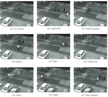
Table4: The definition of nine activities in the BEHAVE dataset.
Activity Definition
In-Group The people are in a group and not moving very much
Approach Two people or groups with one (or both) approaching the other
Walk Together People walking together Ignore Ignoring of one another
Split Two or more people splitting from one another Following Being followed
Meet Two or more people meeting one another Fight Two or more groups fighting
Run together The group is running together
are evaluated. The total number of clusters was 50 for both methods. Letσdbe the standard deviation ofd(xT,vi∗) for all members in a cluster. The value ofσdshould be as small as possible for a more reliable monitoring.Figure 9presents the box-plot that shows the maximum, minimum, median, and the lower and upper quartiles ofσdvalues for the resulting 50 clusters of individual methods. It indicates that the standard FCM method generates a high variation of distances (with a meanσdof 2.93) and the proposed clustering model results in a smaller and more stable variation (with a meanσd of 0.93).
(a1) In-Group
(a4) Ignore
(b1) Meet
(a2) Approach
(a5) Split
(b2) Fight
(a3) Walk Together
(a6) Following
(b3) Run together
Figure10: Activity examples in the BEHAVE dataset: (a1)–(a6) scenarios in the Sequence 0; (b1)–(b3) three activities in Sequence 5, which are abnormal with respect to Sequence.
Table5: The scenarios of the learning and testing sequences for the BEHAVE dataset.
Video clips Scenarios Frame number Video length
Sequence 0 In-Group, Approach, Walk Together, Ignore, Split, Following 1–11200 7 min. 27 sec. Sequence 5 In Group, Approach, Walk Together, Split, Meet, Run Together, Fight 47300–58400 7 min. 24 sec.
473 493 513 533 553 573 584
Frame number ×102
0 5 10 15 20
Δ
d
Meet Fighting
Fighting Running Together
Figure11: Excessive distancesΔdof the four abnormal events in Sequence 5 of the BEHAVE dataset.
The second evaluation dataset is a street scene obtained from the BEHAVE Interactions Test Case Scenarios [56]. BEHAVE is funded by the UK’s Engineering and Physical Science Research Council project. It involves nine different activities such as Walk Together and Run Together in the image sequences. The definitions of these nine activities are listed in Table 4. The BEHAVE dataset has eight video
473 493 513 533 553 573 584
Frame number ×102
0 5 10 15 20
Δ
d Noise
Figure12: Detection results with the 7 moment-based features f1
tof7.
473 493 513 533 553 573 584
Frame number ×102
0 5 10 15 20
Δ
d
Meet Fighting
Fighting Running Together
(a) All features excludingf12
473 493 513 533 553 573 584
Frame number ×102
0 5 10 15 20
Δ
d
(b) All features excludingf10andf11
Figure13: Detection results based on: (a) all features excludingf12;
(b) all features excludingf10and f11.
473 493 513 533 553 573 584
Frame number ×102
0 5 10 15 20
Δ
d
Meet
Incomplete duration of fighting
Fighting Mis-detected
event
Figure 14: Detection results by K-means for Sequence 5 in the BEHAVE dataset.
activities of Meet, Fight, and Run Together are not included in the training sequence 0. Therefore, these three activities are treated as abnormal events. The demonstration images of these three abnormal events are shown inFigure 10(b1)– 10(b3).
The BEHAVE video images are captured at 25 frames per second. The activities and video lengths of the training and testing sequences are listed inTable 5. There are a total of 11,200 frames (7 minutes and 27seconds) in Sequence 0, of which 50% (i.e., 5,600 image frames) are randomly sampled and used as the training samples. The update rate γis set at 0.999 to construct the motion energy maps. The total number of clustersCmax is given by 40. The resulting
minimum control constantβfrom the training process is 0.1. The test video of Sequence 5 has a total of 11,100 frames (7 minutes and 24 seconds).
When the training is done, the whole video images of Sequence 5 are used to test for the detection performance. Figure 11illustrates the testing result of Sequence 5. In the figure, thex-axis presents the frame number and they-axis is the excessive distance Δd. The results show that all the normal activities of In-Group, Approach, Walk Together, and Split in Sequence 5 are within the control limits. There are four major abnormal events detected in Sequence 5, that is, one long fighting event, one short fighting event, one meeting event and one running together event. The resulting
distances of the four abnormal events are distinctly large and prolong for their corresponding durations, as seen in thex-axis and they-axis inFigure 11. The running together event includes many discrete running activities where people abruptly enter and exit from the street scene and, therefore, the resulting distancesΔdare not continuous.
We have also conducted additional experiments on the BEHAVE dataset with various combinations of features. Figure 12 shows the detection results using only the seven moment-based features. It fails to detect the subtle activity of Running Together. Noise is also created. The long Fighting activity is not alarmed at the beginning of the duration, and the overall discrimination magnitudes for the abnormal activities are reduced.
Since feature 12 is the ratio of f10 and f11, we also
evaluate the detection performance without including f12in
the feature set. As seen in Figure 13(a), the four abnormal activities Meet, long Fighting, short Fighting and Running Together are also well detected without the use of feature f12. Comparing the detection results between Figures11and
13(a), the use of 12 full features gives higher discrimination magnitudes, especially in the case of short Fighting. We have also performed the detection task by excluding features f10and f11 (and retaining all the remaining 10 features
for classification).Figure 13(b)shows the detection results. The Running Together event is misdetected, and the whole duration of the long Fighting is not fully detected.
We have also used principal component analysis (PCA) for feature selection. It finds the eigenvalues of the 12 features, and sorts the features in descending order of their corresponding eigenvalues. Then 12 feature sets, each containing the dominant features from 1 to 12, are individually evaluated. The detection results consistently indicate that the use of 12 full features generates the highest discrimination magnitudes. The discrimination power is significantly reduced when less number of features is used for classification.
In order to evaluate the clustering performance between Fuzzy C-means and K-means, we have also used K-means for clustering and classification, and tested it on the BEHAVE dataset. We replicated 10 times with different random initial solutions for both FCM and K-means. Figure 14 shows representative detection results of sequence 5 in the BEHAVE dataset. The K-means technique is less responsive to abnor-mal activities. Compared to the detection results of FCM in Figure 11, K-means clustering procedure misdetects the subtle activity of Running Together. The duration of the long Fighting activity is not fully detected, and the discrimination magnitude of the short Fighting is less significant. Under the same termination criterion, K-means needs additional 40% computation time to converge.
4. Conclusions
detect abnormal events such as burglary and fighting in daily life. The proposed motion energy map can simultaneously represent both spatial context and temporal context of an activity. All historical image frames are taken into account with exponential weights to construct the energy map. It alleviates the limitation on the use of a fixed duration for various activities with different paces. The constrained clustering model can effectively divide numerous activities in daily life into groups based on their similarity in energy maps. By training a sufficient number of randomly sampled energy maps in a video sequence that spans sufficient repetition of day-to-day activities, all normal events can be effectively represented by the cluster centroids. It allows fast computation of similarity measure for each new scene image. The proposed method can therefore be applied for on-line, real-time monitoring of unpredictable abnormal events in daily life.
The merit of this paper is to show the feasibility of the easily-implemented macro-observation approach for abnormality detection in daily life. The proposed scheme in its present form can well detect abnormal events with prolonged durations, especially those lasting tens of seconds or more. It is not highly responsive to the events that last only a few seconds. It is worth further investigation on the spatiotemporal representation and similarity metric for the analysis of short-term activities in daily life.
References
[1] J. Yamato, J. Ohya, and K. Ishii, “Recognizing human action in time sequential images using hidden Markov models,” in Proceedings of the International Conference on Pattern Recognition (ICPR ’92), pp. 379–385, 1992.
[2] R. Polana and R. Nelson, “Low level recognition of human motion (or how to get your man without finding his body parts),” inProceedings of the IEEE Workshop on Motion of Non-Rigid and Articulated Objects, pp. 77–82, Austin, Tex, USA, November 1994.
[3] C. R. Wren, A. Azarbayejani, T. Darrell, and A. P. Pentland, “Pfinder: real-time tracking of the human body,”IEEE Trans-actions on Pattern Analysis and Machine Intelligence, vol. 19, no. 7, pp. 780–785, 1997.
[4] H. Roh, S. Kang, and S.-W. Lee, “Multiple people tracking using an appearance model based on temporal color,” in Pro-ceedings of the International Conference on Pattern Recognition (ICPR ’00), pp. 643–646, 2000.
[5] I. Haritaoglu, D. Harwood, and L. S. Davis, “W4: real-time
surveillance of people and their activities,”IEEE Transactions on Pattern Analysis and Machine Intelligence, vol. 22, no. 8, pp. 809–830, 2000.
[6] Y. Chen, Y. Rui, and T. S. Huang, “JPDAF based HMM for real-time contour tracking,” inProceedings of the IEEE Computer Society Conference on Computer Vision and Pattern Recognition (CVPR ’01), pp. 543–550, December 2001.
[7] I. Haritaoglu, D. Harwood, and L. S. Davis, “Ghost: a human body part labeling system using silhouettes,” inProceedings of the International Conference on Pattern Recognition (ICPR ’98), pp. 77–82, 1998.
[8] T. B. Moeslund and E. Granum, “A survey of computer vision-based human motion capture,”Computer Vision and Image Understanding, vol. 81, no. 3, pp. 231–268, 2001.
[9] C.-W. Chu, O. C. Jenkins, and M. J. Matari´c, “Markerless kine-matic model and motion capture from volume sequences,” in Proceedings of the IEEE Computer Society Conference on Computer Vision and Pattern Recognition (CVPR ’03), pp. 475– 482, June 2003.
[10] G. J. Brostow, I. Essa, D. Steedly, and V. Kwatra, “Novel skeletal representation for articulated creatures,” inProceedings of the 8th European Conference On Computer Vision (ECCV ’04), vol. 3023 ofLecture Notes in Computer Science, pp. 66–79, May 2004.
[11] R. Ishiyama, H. Ikeda, and S. Sakamoto, “A compact model of human postures extracting common motion from individual samples,” inProceedings of the 18th International Conference on Pattern Recognition (ICPR ’06), vol. 1, pp. 187–190, August 2006.
[12] A. Sundaresan and R. Chellappa, “Segmentation and proba-bilistic registration of articulated body models,” inProceedings of the 18th International Conference on Pattern Recognition (ICPR ’06), vol. 2, pp. 92–95, August 2006.
[13] C.-C. Chen, J.-W. Hsieh, Y.-T. Hsu, and C.-Y. Huang, “Seg-mentation of human body parts using deformable triangu-lation,” inProceedings of the 18th International Conference on Pattern Recognition (ICPR ’06), vol. 1, pp. 355–358, August 2006.
[14] R. Navaratnam, A. Thayananthan, P. H. S. Torr, and R. Cipolla, “Hierarchical part-based human body post estimation,” in Proceedings of British Machine Vision Conference (BMVC ’05), pp. 479–488, 2005.
[15] C. Bregler, “Learning and recognizing human dynamics in video sequences,” inProceedings of the IEEE Computer Society Conference on Computer Vision and Pattern Recognition (CVPR ’97), pp. 568–574, June 1997.
[16] Y. Yacoob and M. J. Black, “Parameterized modeling and recognition of activities,”Computer Vision and Image Under-standing, vol. 73, no. 2, pp. 232–247, 1999.
[17] N. M. Oliver, B. Rosario, and A. P. Pentland, “A Bayesian computer vision system for modeling human interactions,” IEEE Transactions on Pattern Analysis and Machine Intelligence, vol. 22, no. 8, pp. 831–843, 2000.
[18] M. Brand and V. Kettnaker, “Discovery and segmentation of activities in video,”IEEE Transactions on Pattern Analysis and Machine Intelligence, vol. 22, no. 8, pp. 844–851, 2000. [19] S. S. Intille and A. F. Bobick, “Recognizing planned,
multiper-son action,”Computer Vision and Image Understanding, vol. 81, no. 3, pp. 414–445, 2001.
[20] H. Buxton, “Learning and understanding dynamic scene activity: a review,”Image and Vision Computing, vol. 21, no. 1, pp. 125–136, 2003.
[21] C. P. Town, “Ontology-driven Bayesian networks for dynamic scene understanding,” inProceedings of the IEEE Computer Society Conference on Computer Vision and Pattern Recognition (CVPR ’04), vol. 7, p. 116, 2004.
[22] A. F. Bobick and A. D. Wilson, “A state-based approach to the representation and recognition of gesture,”IEEE Transactions on Pattern Analysis and Machine Intelligence, vol. 19, no. 12, pp. 1325–1337, 1997.
[23] Q. Dong, Y. Wu, and Z. Hu, “Gesture segmentation from a video sequence using greedy similarity measure,” in Proceed-ings of the 18th International Conference on Pattern Recognition (ICPR ’06), vol. 1, pp. 331–334, August 2006.