Volume 2007, Article ID 92953,24pages doi:10.1155/2007/92953
Research Article
Subspace-Based Noise Reduction for Speech Signals
via Diagonal and Triangular Matrix Decompositions:
Survey and Analysis
Per Christian Hansen1and Søren Holdt Jensen2
1Informatics and Mathematical Modelling, Technical University of Denmark, Building 321, 2800 Lyngby, Denmark
2Department of Electronic Systems, Aalborg University, Niels Jernes Vej 12, 9220 Aalborg, Denmark
Received 1 October 2006; Revised 18 February 2007; Accepted 31 March 2007
Recommended by Marc Moonen
We survey the definitions and use of rank-revealing matrix decompositions in single-channel noise reduction algorithms for speech signals. Our algorithms are based on the rank-reduction paradigm and, in particular, signal subspace techniques. The focus is on practical working algorithms, using both diagonal (eigenvalue and singular value) decompositions and rank-revealing triangular decompositions (ULV, URV, VSV, ULLV, and ULLIV). In addition, we show how the subspace-based algorithms can be analyzed and compared by means of simple FIR filter interpretations. The algorithms are illustrated with working Matlab code and appli-cations in speech processing.
Copyright © 2007 P. C. Hansen and S. H. Jensen. This is an open access article distributed under the Creative Commons Attribution License, which permits unrestricted use, distribution, and reproduction in any medium, provided the original work is properly cited.
1. INTRODUCTION
The signal subspace approach has proved itself useful for signal enhancement in speech processing and many other applications—see, for example, the recent survey [1]. The area has grown dramatically over the last 20 years, along with advances in efficient computational algorithms for ma-trix computations [2–4], especially singular value decompo-sitions and rank-revealing decompodecompo-sitions.
The central idea is to approximate a matrix, derived from the noisy data, with another matrix oflower rankfrom which the reconstructed signal is derived. As stated in [5]:“Rank reduction is a general principle for finding the right trade-off between model bias and model variance when reconstructing signals from noisy data.”
Throughout the literature of signal processing and ap-plied mathematics, these methods are formulated in terms of different notations, such as eigenvalue decompositions, Karhunen-Lo`eve transformations, and singular value de-compositions. All these formulations are mathematically equivalent, but nevertheless the differences in notation can be an obstacle to understanding and using the different methods in practice.
Our goal is to survey the underlying mathematics and present the techniques and algorithms in a common
frame-work and a common notation. In addition to methods based on diagonal (eigenvalue and singular value) decompositions, we survey the use of rank-revealing triangular decomposi-tions. Within this framework, we also discuss alternatives to the classical least-squares formulation, and we show how sig-nals with general (nonwhite) noise are treated by explicit and, in particular, implicit prewhitening. Throughout the paper, we provide small working Matlab codes that illustrate the al-gorithms and their practical use.
We focus onsignal enhancementmethods which directly estimate a clean signal from a noisy one (we do not esti-mate parameters in a parameterized signal model). Our pre-sentation starts with formulations based on (estimated) co-variance matrices, and makes extensive use of eigenvalue de-compositions as well as the ordinary and generalized sin-gular value decompositions (SVD and GSVD)—the latter also referred to as the quotient SVD (QSVD). All these sub-space techniques originate from the seminal 1982 paper [6] by Tufts and Kumaresan, who considered noise reduction of signals consisting of sums of damped sinusoids via linear prediction methods.
Cadzow [7], De Moor [8], Scharf [9], and Scharf and Tufts [5]. Dendrinos et al. [10] used these techniques for speech signals, and Van Huffel [11] applied a similar approach— using the minimum variance estimates from [8]—to expo-nential data modeling. Other applications of these methods can be found, for example, in [1,12–14]. Techniques for gen-eral noise, based on the GSVD, originally appeared in [15], and some applications of these methods can be found in [16–19].
Next we describe computationally favorable alternatives to the SVD/GSVD methods, based on rank-revealing trian-gular decompositions. The advantages of these methods are faster computation and faster up- and downdating, which are important in dynamic signal processing applications. This class of algorithms originates from work by Moonen et al. [20] on approximate SVD updating algorithms, and in par-ticular Stewart’s work on URV and ULV decompositions [21,22]. Some applications of these methods can be found in [23, 24] (direction-of-arrival estimation) and [25] (to-tal least squares). We also describe some extensions of these techniques to rank-revealing ULLV decompositions of pairs of matrices, originating in works by Luk and Qiao [26,27] and Bojanczyk and Lebak [28].
Further extensions of the GSVD and ULLV algorithms to rank-deficient noise, typically arising in connection with narrowband noise and interference, were described in recent work by Zhong et al. [29] and Hansen and Jensen [30,31].
Finally, we show how all the above algorithms can be in-terpreted in terms of FIR filters defined from the decomposi-tions involved [32,33], and we introduce a new analysis tool called “canonical filters” which allows us to compare the be-havior and performance of the subspace-based algorithms in the frequency domain. The hope is that this theory can help to bridge the gap between the matrix notation and more clas-sical signal processing terminology.
Throughout the paper, we make use of the important concept ofnumerical rankof a matrix. The numerical rank of a matrixHwith respect to a given thresholdτis the num-ber of columns ofHthat is guaranteed to be linearly inde-pendent for any perturbation ofHwith norm less thanτ. In practice, the numerical rank is computed as the number of singular values ofH greater thanτ. We refer to [34–36] for motivations and further insight about this issue.
We stress that we do not try to cover all aspects of subspace methods for signal enhancement. For example, we do not treat a number of heuristic methods such as the spectral-domain constrained estimator [12], as well as extensions that incorporate various perceptual constraints [37,38].
Here we have a few words about the notation used throughout the paper:E(·) denotes expectation;R(A) de-notes the range (or column space) of the matrixA;σi(A) de-notes theith singular value ofA;AT denotes the transpose ofA, andA−T =(A−1)T =(AT)−1;I
qis the identity matrix of orderq; andH(v) is the Hankel matrix withncolumns defined from the vectorv(see (4)).
2. THE SIGNAL MODEL
Throughout this paper, we consider only wide-sense station-ary signals with zero mean, and adigital signal is always a column vectors ∈ Rn withE(s) = 0. Associated withsis ann×nsymmetric positive semidefinitecovariance matrix, given byCs≡E(s sT); this matrix has Toeplitz structure, but we do not make use of this property. We will make some im-portant assumptions about the signal.
The noise model
We assume that the signalsconsists of apure signals ∈Rn corrupted byadditive noisee∈Rn,
s=s+e, (1)
and that the noise level is not too high, that is,e2is some-what smaller thans2. In most of the paper, we also assume that the covariance matrix Ce for the noise has full rank. Moreover, we assume that we are able to sample the noise, for example, in periods where the pure signal vanishes (e.g., in speech pauses). We emphasize that the sampled noise vec-toreis not the exact noise vector in (1), but a vector that is statisticallyrepresentativeof the noise.
The pure signal model
We assume that the pure signalsand the noiseeare uncorre-lated, that is,E(seT)=0, and consequently we have
Cs=Cs+Ce. (2)
In the common case whereCe has full rank, it follows that
Cs also has full rank (the case rank(Ce) < n is treated in Section 7). We also assume that the pure signals lies in a propersubspaceofRn; that is,
s∈S⊂Rn, rankCs=dimS=k < n. (3)
The central point in subspace methods is this assumption about the pure signalslying in a (low-dimensional) subspace ofRncalled thesignal subspace. The main goal of all subspace methods is to estimate this subspace and to find a good esti-mates(of the pure signals) in this subspace.
The subspace assumption (which is equivalent to the as-sumption thatCsis rank-deficient) is satisfied, for example, when the signal is a sum of (exponentially damped) sinu-soids. This assumption is perhaps rarely satisfied exactly for a real signal, but it is agood modelfor many signals, such as those arising in speech processing [39].1
For practical computations with algorithms based on the aboven×ncovariance matrices, we need to be able to com-pute estimates of these matrices. The standard way to do this is to assume that we have access todata vectors which are
1It is also a good model for NMR signals [40,41], but these signals are not
longer than the signals we want to consider. For example, for the noisy signal, we assume that we know a data vec-tors ∈ RN with N > n, which allows us to estimate the covariance matrix forsas follows. We note that the lengthN is often determined by the application (or the hardware in which the algorithm is used).
LetH(s) be them×nHankel matrix defined from the vectorsas
H(s)= ⎛ ⎜ ⎜ ⎜ ⎜ ⎜ ⎜ ⎝ s
1 s2 s3 · · · sn
s
2 s3 s4 · · · sn+1
s
3 s4 s5 · · · sn+2 ..
. ... ... ... ...
s
m sm+1 sm+2 · · · sN ⎞ ⎟ ⎟ ⎟ ⎟ ⎟ ⎟ ⎠
(4)
withm+n−1 = N andm ≥ n. Then we define thedata matrixH=H(s), such that we can estimate2the covariance matrixCsby
Cs≈mH1 TH. (5)
Moreover, due to the assumption about additive noise, we haves=s+ewiths,e∈RN, and thus we can write
H=H+E withH=H(s), E=H(e). (6)
Similar to the assumption about Cs, we assume that rank(H)=k.
In broad terms, the goal of our algorithms is to compute an estimatesof the pure signalsfrom measurements of the noisy data vectorsand a representative noise vectore. This is done via a rank-kestimateHof the Hankel matrixH for the pure signal, and we note that we do not require the esti-mateHto have Hankel structure.
There are several approaches to extracting a signal vector from them×nmatrixH. One approach, which produces a length-Nvectors, is toaveragealong the antidiagonals ofH, which we write as
s=A(H)∈RN. (7)
The corresponding Matlab code is
shat = zeros(N,1); for i=1:N
shat(i) = mean(diag(fliplr(Hhat),n-i)); end
This approach leads to the FIR filter interpretation in Section 9. The rank-reduction + averaging process can be it-erated, and Cadzow [7] showed that this process converges to a rank-kHankel matrix; however, De Moor [42] showed that this may not be the desired matrix. In practice, the single averaging in (7) works well.
2 Alternatively, we could work with the Toeplitz matrices obtained by
reversing the order of the columns of the Hankel matrices; all our rela-tions will still hold.
0 50 100 150 200 Sample number
−0.2 0 0.2
Amp
li
tu
d
e
Clean
(a)
0 50 100 150 200 Sample number
−0.2 0 0.2
Amp
li
tu
d
e
White
(b)
0 50 100 150 200 Sample number
−0.2 0 0.2
Amp
li
tu
d
e
Colored
(c)
Figure1: The three signals of lengthN =240 used in our
exam-ples. (a) Clean speech signal (voiced segment of male speaker); (b) white noise generated by Matlab’srandnfunction; (c) colored noise (segment of a recording of strong wind). The clean signal slightly vi-olates the subspace assumption (3), seeFigure 3.
Doclo and Moonen [1] found that the averaging oper-ation is often unnecessary. An alternative approach, which produces a length-nvector, is therefore to simplyextract(and transpose) an arbitrary row of the matrix, that is,
s=H(, :)T∈Rn, arbitrary. (8)
This approach lacks a solid theoretical justification, but due to its simplicity it lends itself well to the up- and downdating techniques in dynamical processing, seeSection 8.
Speech signals can, typically, be considered stationary in segments of length up to 30 milliseconds, and for this rea-son it is a common practice to process speech signals in such segments—either blockwisely (normally with overlap between the block) or using a “sliding window” approach.
Throughout the paper, we illustrate the use of the sub-space algorithms with a 30 milliseconds segment of a voiced sound from a male speaker recorded at 8 kHz sampling fre-quency of lengthN=240. The algorithms also work for un-voiced sound segments, but the un-voiced sound is better suited for illustrating the performance.
usem=211 andn=30, and the signal-to-noise ratio in the noisy signals, defined as
SNR=20 log
s 2
e2
dB, (9)
is 10 dB unless otherwise stated.
When displaying the spectrum of a signal, we always use the LPC power spectrum computed with Matlab’slpc func-tion with order 12, which is standard in speech analysis of signals sampled at 8 kHz.
3. WHITE NOISE: SVD METHODS
To introduce ideas, we consider first the ideal case of white noise, that is, the noise covariance matrix is a scaled identity,
Ce=η2In, (10)
whereη2is the variance of the noise. The covariance matrix for the pure signal has the eigenvalue decomposition
Cs=VΛVT, Λ=diagλ1,. . .,λn
(11)
withλk+1 = · · · = λn = 0. The covariance matrix for the noisy signal,Cs=Cs+η2In, has the same eigenvectors while its eigenvalues areλi+η2(i.e., they are “shifted” byη2). It follows immediately that givenηand the eigenvalue decom-position ofCs, we can perfectly reconstructCssimply by sub-tractingη2from the largestkeigenvalues ofC
sand inserting these in (11).
In practice, we cannot design a robust algorithm on this simple relationship. For one thing, the rankkis rarely known in advance, and white noise is a mathematical abstraction. Moreover, even if the noiseeis close to being white, a prac-tical algorithm must use an estimate of the varianceη2, and there is a danger that we obtain some negative eigenvalues when subtracting the variance estimate from the eigenvalues ofCs.
A more robust algorithm is obtained by replacingkwith anunderestimateof the rank, and by avoiding the subtraction ofη2. The latter is justified by a reasonable assumption that the largestkeigenvaluesλi,i=1,. . .,k, are somewhat greater thanη2.
A working algorithm is now obtained by replacing the covariance matrices with their computable estimates. For both pedagogical and computational/algorithmic reasons, it is most convenient to describe the algorithm in terms of the two SVDs:
H=UΣVT =U1U2 Σ1 0
0 0
V1,V2 T
, (12)
H=UΣVT =U 1,U2
Σ1 0 0 Σ2
V1,V2 T
, (13)
in whichU,U∈Rm×nandV,V ∈Rn×nhave orthonormal columns, andΣ,Σ ∈Rn×nare diagonal. These matrices are partitioned such thatU1,U1 ∈ Rm×k,V1,V1 ∈ Rn×k, and
Σ1,Σ1∈Rk×k. We note that the SVDs immediately provide
the eigenvalue decompositions of the cross-product matri-ces, because
HTH=VΣ2
VT, HTH=VΣ2VT. (14)
The pure signal subspace is then given byS =R(V1), and our goal is to estimate this subspace and to estimate the pure signal via a rank-kestimateHof the pure-signal matrixH.
Moving from the covariance matrices to the use of the cross-product matrices, we must make further assumptions [8], namely (in the white-noise case) that the matricesEand
Hsatisfy
1
mETE=η2In, HTE=0. (15)
These assumptions are stronger thanCe=η2I
nandE(s eT)= 0. The first assumption is equivalent to the requirement that the columns of (√mη)−1Eare orthonormal. The second as-sumption implies the requirement thatm≥n+k.
Then it follows that
1
mHTH=
1
mHTH+η2In (16)
and if we insert the SVDs and multiply withm, we obtain the relation
V1,V2
Σ2
1 0
0 Σ2 2
V1,V2
T
=V1,V2 Σ2
1+mη2Ik 0
0 mη2I
n−k
V1,V2 T
,
(17)
whereIkandIn−kare identity matrices. From the SVD ofH, we can then estimatekas the numerical rank ofHwith re-spect to the threshold m1/2η. Furthermore, we can use the subspaceR(V1) as an estimate ofS(see, e.g., [43] for results about the quality of this estimate under perturbations).
We now describe several empirical algorithms for com-puting the estimate H; in these algorithms k is always the numerical rank ofH. The simplest approach is to compute
Hls as a rank-kleast-squares estimateofH, that is,Hlsis the closest rank-kmatrix toHin the 2-norm (and the Frobenius norm),
Hls=argminHH−H 2 s.t. rank(H)=k. (18)
The Eckart-Young-Mirsky theorem (see [44, Theorem 1.2.3] or [2, Theorem 2.5.3]) expresses this solution in terms of the SVD ofH:
Hls=U1Σ1V1T. (19)
If desired, it is easy to incorporate the negative “shift” men-tioned above. It follows immediately from (17) that
Σ2
1=Σ21−mη2Ik=
Ik−mη2Σ−12
Σ2
which leads Van Huffel [11] to defines a modified least-squares estimate:
Hmls=U1ΦmlsΣ1V1T withΦmls=
Ik−mη2Σ−12 1/2
.
(21)
The estimate s from this approach is an empirical least-squares estimate ofs.
A number of alternative estimates have been proposed. For example, De Moor [8] introduced theminimum variance estimateHmv=HWmv, in whichWmvsatisfies the criterion
Wmv=argminWH−HWmvF, (22)
and he showed (see our appendix) that this estimate is given by
Hmv=U1ΦmvΣ1V1T withΦmv=Ik−mη2Σ−12. (23)
Ephraim and Van Trees [12] defined atime-domain con-straint estimatewhich, in our notation, takes the formHtdc=
HWtdc, whereWtdcsatisfies the criterion
Wtdc=argminWH−HWF s.t.WF≤α
√
m, (24)
in whichαis a user-specified positive parameter. If the con-straint is active, then the matrixWtdcis given by the Wiener solution3
Wtdc=V1Σ 2 1
Σ2
1+λmη2Ik −1
VT1, (25)
where λis the Lagrange parameter for the inequality con-straint in (24). If we use (17), then we can write the TDC estimate in terms of the SVD ofHas
Htdc=U1ΦtdcΣ1V1T withΦtdc=
Ik−mη2Σ−12
·Ik−mη2(1−λ)Σ−12 −1
.
(26)
This relation is derived in our appendix. If the constraint is inactive, thenλ=0 and we obtain the LS solution. Note that we obtain the MV solution forλ=1.
All these algorithms can be written in a unified formula-tion as
Hsvd=U1ΦΣ1V1T, (27)
whereΦis a diagonal matrix, called thegain matrix, deter-mined by the optimality criterion, seeTable 1. Other choices ofΦare discussed in [45]. The corresponding Matlab code for the MV estimate is
[U,S,V] = svd(H,0);
k = length(diag(S) > sqrt(m)*eta);
Phi = eye(k) - m*eta^2*inv(S(1:k,1:k)^2); Hhat = U(:,1:k)*Phi*S(1:k,1:k)*V(:,1:k)’;
3In the regularization literature,W
tdc is known as a Tikhonov solution
[34].
Table1: Overview of some important gain matrixΦin the
SVD-based methods for the white noise case.
Estimate Gain matrixΦ
LS Ik
MLS Ik−mη2Σ−12
1/2
MV Ik−mη2Σ−12
TDC Ik−mη2Σ−12
·Ik−mη2(1−λ)Σ−12 −1
with the codes for the other estimates being almost similar (only the expression forPhichanges).
A few practical remarks are in order here. The MLS, MV, and TDC methods require knowledge about the noise vari-anceη2; good estimates of this quantity can be obtained from samples of the noiseein the speech pauses. The thresholds used in all our Matlab templates (here, τ = √mη) are the ones determined by the theory. In practice, we advice the inclusion of a “safety factor,” say,√2 or 2, in order to ensure thatkis an underestimate (because overestimates included noisy components). However, since this factor is somewhat problem-dependent, it is not included in our templates.
We note that (27) can also be written as
Hsvd=HWΦ, WΦ=V
Φ 0
0 0
VT, (28)
whereWΦis a symmetric matrix which takes care of both the truncation atk, and the modification of the singular values (WΦis a projection matrix in the LS case only). Using this formulation, we immediately see that the estimates(8) takes the simple form
s=WΦH(, :)T =WΦs, (29)
wheresis an arbitrary length-nsignal vector. This approach is useful when the signal is quasistationary for longer periods, and the same filter, determined byWΦ, can be used over these periods (or in an exponential window approach).
4. RANK-REVEALING TRIANGULAR DECOMPOSITIONS
In real-time signal processing applications, the computa-tional work in the SVD-based algorithms, both in computing and updating the decompositions, may be too large. Rank-revealing triangular decompositions are computationally at-tractive alternatives which are faster to compute than the SVD, because they involve an initial factorization that can take advantage of the Hankel structure, and they are also much faster to update than the SVD. For example, computa-tion of the SVD requiresO(mn2) flops while a rank-revealing triangular decomposition can be computed inO(mn) flops if the structure is utilized. Detailed flop counts and compar-isons can be found in [25,46].
Pack [48]. These packages include software for efficient com-putation of all the decompositions, as well as software for up-and downdating. The software is designed such that one can either estimate the numerical rank or use a fixed predeter-mined value fork.
4.1. UTV decompositions
Rank-revealing UTV decompositions were introduced in the early 1990s by Stewart [21,22] as alternatives to the SVD, and they take the forms (referred to as URV and ULV, resp.)
H=UR
R11 R12
0 R22
VT R,
H=UL
L11 0
L21 L22
VT L,
(30)
whereR11,L11∈Rk×k. We will adopt Pete Stewart’s notation
T(for “triangular”) for eitherLorR.
The four “outer” matricesUL,UR ∈Rm×n, andVL,VR∈
Rn×nhavenorthonormal columns, and the numerical rank4 ofHis revealed in the middlen×ntriangular matrices:
σiR11
≈σiL11
≈σi(H), i=1,. . .,k,
R12
R22 F
≈L21,L22F≈σk+1(H).
(31)
In our applications, we assume that there is a well-defined gap betweenσk andσk+1. The more work one is willing to spend in the UTV algorithms, the smaller the norm of the off-diagonal blocksR12andL21is.
In addition to information about numerical rank, the UTV decompositions also provide approximations to the SVD subspaces, (cf. [34, Section 3.3]). For example, ifVR1=
VR(:, 1 :k), then the subspace angle∠(V1,VR1) between the ranges ofV1(in the SVD) andVR1(in the URV decomposi-tion) satisfies
sin∠V1,VR1
≤ σk
R11R122
σkR11 2
−R2222
. (32)
The similar result forVL1 =VL(:, 1 :k) in the ULV decom-position takes the form
sin∠V1,VL1
≤ L212L222
σkL11 2
−L2222
. (33)
We see that the smaller the norm ofR12andL21is, the smaller the angle is. The ULV decomposition can be expected to give better approximations to the signal subspace R(V1) than URV when there is a well-defined gap betweenσkandσk+1,
4 The case whereHis exactly rank-deficient, for which the submatrices R12,R22,L21, andL22are zero, was treated much earlier by Golub [49] in
1965.
Table2: Symmetric gain matrixΨfor UTV and VSV (for the white
noise case), using the notationT11for eitherR11,L11, orS11.
Estimate Gain matrixΨ
LS Ik
MV Ik−mη2T11−1T11−T
TDC Ik−mη2T11−1T11−T
·Ik−mη2(1−λ)T−1
11T11−T
−1
due to the factorsσk(R11)≈ σkandL222 ≈σk+1in these bounds.
For special cases where the off-diagonal blocksR12 and
L21 are zero, and under the assumption that σk(T11) >
T222—in which case R(VT1) = R(V1)—we can derive explicit formulas for the estimators fromSection 3. For ex-ample, the least-squares estimates are obtained by simply neglecting the bottom blockT22—similar to neglecting the blockΣ2in the SVD approach. The MV and TDC estimates are derived in the appendix.
In practice, the off-diagonal blocks are not zero but have small norm, and therefore it is reasonable to also neglect these blocks. In general, our UTV-based estimates thus take the form
Hutv=UT
T11Ψ 0
0 0
VT
T, (34)
where the symmetric gain matrixΨis given inTable 2. The MV and TDC formulations, which are derived by replacing the matrix inΣ2
1inTable 1withT11TT11, were originally pre-sented in [50,51], respectively; there is no estimate that cor-responds to MLS. We emphasize again that these estimators only satisfy the underlying criterion when the off-diagonal block is zero.
In analogy with the SVD-based methods, we can use the alternative formulations
Hurv =HWR,Ψ, Hulv=HWL,Ψ (35) with the symmetric matrixWT,Ψgiven by
WT,Ψ=VT
Ψ 0
0 0
VT
T. (36)
The two estimatesHulvandHulvare not identical; they differ byUL(:,k+1 :n)L21VL(:, 1 :k)T whose normL212is small. The Matlab code for the ULV case with high rank (i.e.,
k≈n) takes the form
[k,L,V] = hulv(H,eta); Ik = eye(k);
Psi = Ik - m*eta^2*...
L(1:k,1:k)\Ik/L(1:k,1:k)’; Hhat = H*V(:,1:k)*Psi*V(:,1:k)’;
An alternative code that requires more storage forUhas the form
[k,L,V,U] = hulv(H,eta); Psi = Ik - m*eta^2*...
L(1:k,1:k)\Ik/L(1:k,1:k)’;
For the ULV case with low rank (k n), changehulvto
lulv, and for the URV cases change ulvto urv.
4.2. Symmetric VSV decompositions
If the signal lengthNis odd and we usem=n(ignoring the conditionm≥n+k), then the square Hankel matricesHand
Eare symmetric. It is possible to utilize this property in both the SVD and the UTV approaches.
In the former case, we can use that a symmetric matrix has the eigenvalue decomposition
H=VΛVT (37)
with real eigenvalues inΛand orthonormal eigenvectors in
V, and thus the SVD ofHcan be written as
H=VD|Λ|VT, D=diagsignλ
i. (38)
This well-known result essentially halves the work in com-puting the SVD. The remaining parts of the algorithm are the same, using|Λ|forΣ.
In the case of triangular decompositions, a symmetric matrix has a symmetric rank-revealing VSV decomposition of the form
H=VS
S11 S12
ST 12 S22
VT
S, (39)
where VS ∈ Rn×n is orthogonal, and S11 ∈ Rk×k and S22 are symmetric. The decomposition is rank-revealing in the sense that the numerical rank is revealed in the “middle”n×n symmetric matrix:
σiS11
≈σi(H), i=1,. . .,k,
S12
S22
F≈σk+1
(H). (40)
The symmetric rank-revealing VSV decomposition was orig-inally proposed by Luk and Qiao [52], and it was further de-veloped in [53].
The VSV-based matrix estimate is then given by
Hvsv=VS
S11Ψ 0
0 0
VT
S, (41)
in which the gain matrixΨis computed fromTable 2with
T11 replaced by the symmetric matrixS11. Again, these ex-pressions are derived under the assumption thatS12 =0; in practice the norm of this block is small.
The algorithms in [53] for computing VSV decomposi-tions return a factorization ofSwhich, in the indefinite case, takes the form
S=TTΩT, (42)
where T is upper or lower triangular, and Ω = diag(±1).
Below is Matlab code for the high-rank case (k≈n):
[k,R,Omega,V] = hvsvid_R(A,eta); Ik = eye(k);
M = R(1:k,1:k)’\Ik/R(1:k,1:k); M = Omega(1:k,1:k)*M*Omega(1:k,1:k); Psi = Ik - R(1:k,1:k)\M/R(1:k,1:k)’; Hhat = V(:,1:k)*S(1:k,1:k)*Psi*V(:,1:k)’;
5. WHITE NOISE EXAMPLE
We start with an illustration of the noise reduction for the white noise case by means of SVD and ULV, using an artifi-cially generated clean signal:
si=sin(0.4i) + 2 sin(0.9i) + 4 sin(1.7i) + 3 sin(2.6i) (43) fori = 1,. . .,N. This signal satisfies the subspace assump-tion, and the corresponding clean data matrixHhas rank 8. We add white noise with SNR=0 dB (to emphasize the influence of the noise), and we compute SVD and ULV LS-estimates fork = 1,. . ., 9.Figure 2shows LPC spectra for each signal, and we see that the two algorithms produce very similar results.
This example illustrates that askincreases, we include an increasing number of spectral components, and this occurs in the order of decreasing energy of these components. It is precisely this behavior of the subspace algorithms that makes them so powerful for signals that (approximately) admit the subspace model.
We now turn to the speech signal fromFigure 1, recall-ing that this signal does not satisfy the subspace assumption exactly.Figure 3shows the singular values of the two Hankel matricesHandHassociated with the clean and noisy signals. We see that the larger singular values ofH are quite similar to those ofH, that is, they are not affected very much by the noise—while the smaller singular values of H tend to level offaround√mη, which is the variance of the noise.Figure 3 also shows our “safeguarded” threshold√2√mηfor the trun-cation parameter, leading to the choicek =13 for this par-ticular realization of the noise.
The rank-revealing UTV algorithms are designed such that they reveal the large and small singular values ofH in the triangular matricesRandL, andFigure 4shows a clear grading of the size of the nonzero elements in these matri-ces. The particular structure of the nonzero elements inR andL depends on the algorithm used to compute the de-composition. We see that the “low-rank versions”lurvand
lulvtend to produce triangular matrices whose off-diagonal blocksR12andL21have smaller elements than those from the “high-rank versions”hurvandhulv(see [47] for more de-tails about these algorithms).
Next we illustrate the performance of the SVD- and ULV-based algorithms using the minimum-variance (MV) esti-mates.Figure 5(a) shows the LPC spectra for the clean and noisy signals—in the clean signal we see four distinct for-mants, while only two formants are above the noise level in the noisy signal.
0 1000 2000 3000 Frequency (Hz) −10 0 10 20 30 Ma gn it u d e (d B ) Pure signal Noisy signal (a)
0 1000 2000 3000
Frequency (Hz) −10 0 10 20 30 Ma gn it u d e (d B ) Pure signal SVD estimate ULV estimate k=1
(b)
0 1000 2000 3000
Frequency (Hz) −10 0 10 20 30 Ma gn it u d e (d B ) Pure signal SVD estimate ULV estimate k=2
(c)
0 1000 2000 3000
Frequency (Hz) −10 0 10 20 30 Ma gn it u d e (d B ) Pure signal SVD estimate ULV estimate k=3
(d)
0 1000 2000 3000
Frequency (Hz) −10 0 10 20 30 Ma gn it u d e (d B ) Pure signal SVD estimate ULV estimate k=4
(e)
0 1000 2000 3000
Frequency (Hz) −10 0 10 20 30 Ma gn it u d e (d B ) Pure signal SVD estimate ULV estimate k=5
(f)
0 1000 2000 3000
Frequency (Hz) −10 0 10 20 30 Ma gn it u d e (d B ) Pure signal SVD estimate ULV estimate k=6
(g)
0 1000 2000 3000
Frequency (Hz) −10 0 10 20 30 Ma gn it u d e (d B ) Pure signal SVD estimate ULV estimate k=7
(h)
0 1000 2000 3000
Frequency (Hz) −10 0 10 20 30 Ma gn it u d e (d B ) Pure signal SVD estimate ULV estimate k=8
(i)
0 1000 2000 3000
Frequency (Hz) −10 0 10 20 30 Ma gn it u d e (d B ) Pure signal SVD estimate ULV estimate k=9
(j)
Figure2: Example with a sum-of-sines clean signal for whichHhas rank 8, and additive white noise with SNR 0 dB. Top left: LPC spectra
0 5 10 15 20 25 30 Indexi
100
101
σi
σi(noisy signal) σi(clean signal)
τm1/2η
m1/2η
Figure3: The singular values of the Hankel matricesH(clean
sig-nal) andH (noisy signal). The solid horizontal line is the “safe-guarded” threshold√2m1/2η; the numerical rank with respect to
this threshold isk=13.
parametersk = 8 andk = 16, respectively. Note that the SVD- and ULV-estimates have almost identical spectra for a fixedk, illustrating the usefulness of the more efficient ULV algorithm. Fork = 8, the two largest formants are well re-constructed; butkis too low to allow us to capture all four formants. Fork=16, all four formants are reconstructed sat-isfactorily, while a larger value ofkleads to the inclusion of too much noise. This illustrates the importance of choosing the correct truncation parameter. The clean and estimated signals are compared inFigure 6.
6. GENERAL NOISE
We now turn to the case of more general noise whose covari-ance matrixCeis no longer a scaled identity matrix. We still assume that the noise and the pure signal are uncorrelated and thatCehas full rank. LetCehave the Cholesky factoriza-tion
Ce=RTeRe, (44)
whereReis an upper triangular matrix of full rank. Then the standard approach is to consider the transformed signalR−eTs whose covariance matrix is given by
ER−T e s sTR−e1
=R−T
e CsR−e1=Re−TCsR−e1+In, (45)
showing that the transformed signal consists of a trans-formed pure signal plus additive white noise with unit vari-ance. Hence the name prewhitening is used for this pro-cess. Clearly, we can apply all the methods from the previ-ous section to this transformed signal, followed by a back-transformation involving multiplication withRTe.
Turning to practical algorithms based on the cross-product matrix estimates for the covariance matrices, our as-sumptions are now
rank(E)=n, HTE=0. (46)
SinceEhas full rank, we can compute an orthogonal factor-izationE=QRin whichQhas orthonormal columns andR
is nonsingular. For example, if we use aQRfactorization then
Ris a Cholesky factor ofETE, andm−1/2RestimatesR eabove. We introduce the transformed signalzqr =R−Tswhose co-variance matrix is estimated by
1
mR−THTHR−1=
1
mR−THTHR−1+
1
mIn, (47)
showing that the prewhitened signal zqr—similar to the above—consists of a transformed pure signal plus additive white noise with variancem−1. Again we can apply any of the methods from the previous section to the transformed sig-nalzqr, represented by the matrixZqr=HR−1, followed by a back-transformation withRT.
The complete model algorithm for treating full-rank nonwhite noise thus consists of the following steps. First, compute the QR factorization E = QR, then form the prewhitened matrixZqr=H R−1and compute its SVDZqr=
UΣVT. Then compute the “filtered” matrix Z
qr = ZqrWΦ with the gain matrixΦfromTable 1usingmη2=1. Finally, compute the dewhitened matrixHqr =ZqrRand extract the filtered signal. For example, for the MV estimate this is done by the following Matlab code:
[Q,R] = qr(E,0); [U,S,V] = svd(H/R,0);
k = length(diag(S) > 1/sqrt(m)); Phi = eye(k) - inv(S(1:k,1:k))^2; Hhat = U(:,1:k)*Phi*S(1:k,1:k)...
*V(:,1:k)’*R;
6.1. GSVD methods
There is a more elegant version of the above algorithm which avoids the explicit pre- and dewhitening steps, and which can be extended to a rank-deficientE, (cf.Section 7). It can be formulated both in terms of the covariance matrices and their cross-product estimates.
Consider first the covariance matrix approach [16,17], which is based on the generalized eigenvalue decomposition ofCsandCe:
Cs=XΛXT, Ce=X XT, (48)
whereΛ = diag(λ1,. . .,λn) andX is a nonsingular matrix5 (see, e.g., [2, Section 8.7]). If we partitionX = (X1,X2) with X1 ∈ Rn×k, then the pure signal subspace satisfies
S=R(X1). Moreover,
Cs=Cs+Ce=XΛ+InXT, (49)
showing that we can perfectly reconstructCs(similar to the white noise case) by subtracting 1 from theklargest general-ized eigenvalues ofCs.
10 20 30 30
25 20 15 10 5
−3 −2 −1 0 1 hurv: log10|R|
(a)
10 20 30
30 25 20 15 10 5
−3 −2 −1 0 1 hurv: log10|R|
(b)
10 20 30
30 25 20 15 10 5
−3 −2 −1 0 1 lulv: log10|L|
(c)
10 20 30
30 25 20 15 10 5
−3 −2 −1 0 1 hulv: log10|L|
(d)
Figure4: The large and small singular values are reflected in the size of the elements in the matricesRandLfrom the URV and ULV
decompositions. The triangular matrices from thelurvandlulvalgorithms (left plots) are closer to block diagonal form than those from thehurvandhulvalgorithms (right plots).
As demonstrated in [15], we can turn the above into a working algorithm by means of the generalized SVD (GSVD) ofHandE, given by
H=UHΓXT, E=UEΔXT. (50)
IfEhas full rank, thenX ∈Rn×nis nonsingular. Moreover,
UH,UE∈Rm×nhave orthonormal columns, andΓ,Δ∈Rn×n are diagonal matrices
Γ=diagγ1,. . .,γn
, Δ=diagδ1,. . .,δn
(51)
satisfyingΓ2+Δ2=I(see, e.g., [44, Section 4.2]). In theQR -based algorithm described above, we now replace theQR fac-torization ofEwith the factorizationE=UE(ΔXT), leading to a matrixZgsvdgiven by
Zgsvd=H
ΔXT−1
=UHΓΔ−1, (52)
which is the SVD ofZgsvd expressed in terms of GSVD fac-tors. The corresponding signalzgsvd=(ΔXT)−Ts=(XΔ)−1s
consists of the transformed pure signal (XΔ)−1splus addi-tive white noise with variance m−1. Also, the pure signal subspace is spanned by the first k columns of X, that is,
S=R(X(:, 1 :k)).
LetΓ1andΔ1denote the leadingk×ksubmatrices ofΓ andΔ. Then the filtered and dewhitened matrixHgsvdtakes the form
Hgsvd=UHΓ
Φ 0 0 0
XT =HYΦ (53)
with
YΦ=X−T
Φ 0
0 0
XT, (54)
where againΦis fromTable 1 withΣ1 = Γ1Δ−11 = Γ1(I −
Γ2
1)−1/2andmη2=1. Thus we can compute the filtered signal either by averaging along the antidiagonals ofHgsvdor as
0 500 1000 1500 2000 2500 3000 3500 4000 Frequency (Hz)
−40 −30 −20 −10 0
M
ag
nitude
(dB)
Pure signal Noisy signal
(a)
0 500 1000 1500 2000 2500 3000 3500 4000 Frequency (Hz)
−40 −30 −20 −10 0
M
ag
nitude
(dB)
Pure signal SVD estimate,k=8 ULV estimate,k=8
(b)
0 500 1000 1500 2000 2500 3000 3500 4000 Frequency (Hz)
−40 −30 −20 −10 0
M
ag
nitude
(dB)
Pure signal SVD estimate,k=16 ULV estimate,k=16
(c)
Figure5: LPC spectra of the signals in the white noise example,
us-ing SVD- and ULV-based MV estimates. (a) Clean and noisy signals; (b) and (c) estimates; both SNRs are 12.5 dB fork=8 and 13.8 dB fork=16.
The Matlab code for MV case takes the form
[U,V,X,Gamma,Delta] = gsvd(H,E,0); S = Gamma/Delta;
k = length(diag(S) > 1);
Phi = eye(k) - inv(S(1:k,1:k))^2; Hhat = U(:,1:k)*Gamma(1:k,1:k)...
*Phi*X(:,1:k)’;
We note that if we are given (an estimate of) the noise covariance matrixCe instead of the noise matrixE, then in
0 50 100 150 200
Sample number −0.9
0 0.9
A
m
plitude
Clean SVD,k=16
Figure6: Comparison of the clean signal and the SVD-based MV
estimate fork=16.
the GSVD-based algorithm we can replace the matrixEwith the Cholesky factorRein (44).
6.2. Triangular decompositions
Just as the URV and ULV decompositions are alternatives to the SVD—with a middle triangular matrix instead of a middle diagonal matrix—there are alternatives to the GSVD with middle triangular matrices. They also come in two ver-sions with upper and lower triangular matrices but, as shown in [30], only the version using lower triangular matrices is useful in our applications.
This version is known as the ULLV decomposition ofH andE; it was introduced by Luk and Qiao [26] and it takes the form
H=UHLHLVT, E=UELVT, (56)
whereLH,L∈Rn×nare lower triangular, and the three ma-trices UH,UE ∈ Rm×n andV ∈ Rn×n have orthonormal columns. See [50,51] for applications of the ULLV decom-position in speech processing.
The prewhitening technique fromSection 6carries over to the ULLV decomposition. Using the orthogonal decompo-sition ofEin (56), we define the transformed (prewhitened) signalzullv =(LVT)−Ts=L−TVTswhose scaled covariance matrix is estimated by (1/m)ZullvT Zullv, in which
Zullv=H
LVT−1
=UHLH, (57)
and we see that the ULLV decomposition automatically pro-vides a ULV decomposition of this matrix. Hence we can use the techniques fromSection 4.1to obtain the estimate
Zullv=UH
LH,11Ψ 0
0 0
, (58)
whereLH,11denotes the leadingk×ksubmatrix ofLH. This leads to the ULLV-based estimate
Hullv=ZullvLVT=UH
LH,11Ψ 0
0 0
LVT. (59)
The alternative version takes the form
Hullv=HYΨ withYΨ=VL−1
Ψ 0
0 0
and the gain matrixΨis given by the expressions inTable 2 withT11replaced byLH,11andmη2=1. The Matlab code for the MV estimate is
[k,LH,L,V,UH] = ullv(H,E,1); Ik = eye(k);
Psi = Ik - LH(1:k,1:k)\Ik/LH(1:k,1:k)’; Hhat = UH(:,1:k)*LH(1:k,1:k)...
*Psi*L(1:k,1:k)*V(:,1:k)’;
Similar to the GSVD algorithm, we can replace E by the Cholesky factorReof the noise covariance matrix in (44), if it is available.
6.3. Colored noise example
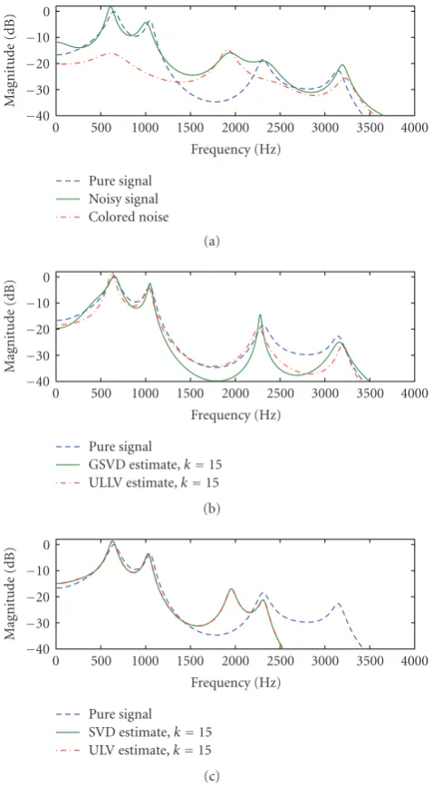
We now switch to the colored noise (the wind signal), and Figure 7(a) shows the power spectra for the pure and noisy signals, together with the power spectrum for the noise sig-nal which is clearly nonwhite.Figure 7(b) shows the power spectra for the MV estimates using the GSVD and ULLV al-gorithms withk =15; the corresponding SNRs are 12.1 dB and 11.4 dB. The GSVD estimate is superior to the ULLV es-timate, but both give a satisfactory reduction of the noise in the frequency ranges between and outside the formants. The GSVD-based signal estimate is compared with the clean sig-nal inFigure 8.
Figure 7(c) illustrates the performance of the SVD and ULV algorithms applied to this signal (i.e., there is no pre-conditioning). Clearly, the implicit white noise assumption is not correct and the estimates are inferior to those using the GSVD and ULLV algorithms because the SVD and ULV algorithms mistake some components of the colored noise for signal.
7. RANK-DEFICIENT NOISE
Not all noise signals lead to a full-rank noise matrixE; for example, narrowband signals often lead to anEthat is (nu-merically) rank-deficient. In this case, we may think of the noise as an interfering signal that we need to suppress.
WhenEis rank-deficient, the above GSVD- and ULLV-based methods do not apply becauseΔandLbecome deficient. In [31], we extended these algorithms to the rank-deficient case; we summarize the algorithms here, and refer to the paper for the—quite technical—details.
The GSVD is not unique in the rank-deficient case, and several formulations appear in the literature. We use the for-mulation in Matlab, and our algorithms require an initial rank-revealingQRfactorization ofEof the form
E=QR, R∈Rp×n, (61)
whereRis upper trapezoidal andp=rank(E). Then we use a GSVD of (H,R) of the form
H=UH
Γ 0 0 Io
XT,
R=UR(Δ, 0)XT,
(62)
0 500 1000 1500 2000 2500 3000 3500 4000 Frequency (Hz)
−40 −30 −20 −10 0
M
ag
nitude
(dB)
Pure signal Noisy signal Colored noise
(a)
0 500 1000 1500 2000 2500 3000 3500 4000 Frequency (Hz)
−40 −30 −20 −10 0
M
ag
nitude
(dB)
Pure signal
GSVD estimate,k=15 ULLV estimate,k=15
(b)
0 500 1000 1500 2000 2500 3000 3500 4000 Frequency (Hz)
−40 −30 −20 −10 0
M
ag
nitude
(dB)
Pure signal SVD estimate,k=15 ULV estimate,k=15
(c)
Figure 7: LPC spectra of the signals in the colored-noise
exam-ple, using the MV estimates. (a) Clean and noisy signals together with the noise signal; (b) GSVD and ULLV estimates; the SNRs are 12.1 dB and 11.4 dB; (c) SVD and ULV estimates (both SNRs are 11.4 dB). Without knowledge about the noise, the SVD and ULV methods mistake some components of the colored noise for a sig-nal.
0 50 100 150 200
Sample number −0.9
0 0.9
A
m
plitude
Clean GSVD,k=15
Figure8: Comparison of the clean signal and the GSVD-based MV
whereΓandΔarep×pand diagonal, andIois the identity matrix of ordern−p. Moreover,UH∈Rm×nandUR∈Rp×p have orthonormal columns, andX∈Rn×nis nonsingular.
The basic idea in our algorithm is to realize that there is no noise in the subspaceR(X(:,p+1 :n)) spanned by the last
n−kcolumns ofX, and therefore any component of the noisy signalsin this subspace should not be filtered. The filtering should only take place in the subspaceR(X(:, 1 : p)). Note that the vectors in these two subspaces are not orthogonal; as shown in [30], orthogonal subspaces are inferior to the bases
X(:, 1 :p) andX(:,p+1 :n).
Again letΓ1andΔ1denote the leadingk×ksubmatrices ofΓandΔ. Then the GSVD-based estimate takes the form
Hgsvd=UH
Γ 0 0 Io
⎛ ⎜ ⎜ ⎝
Φ 0 0
0 0 0
0 0 Io
⎞ ⎟ ⎟
⎠XT, (63)
where, similar to the full-rank case, thek×kgain matrixΦis fromTable 1withΣ1=Γ1Δ−11=Γ1(I−Γ21)−1/2andmη2=1. The corresponding Matlab code for the MV estimate, which requires UTV Tools for the rank-revealingQR factor-izationhrrqr, takes the form (wherethris the threshold for the rank decision inE)
thr = 1e-12*norm(E,’fro’); [Q,R] = hrrqr(E,thr);
[UH,UR,X,Gamma,Delta] = gsvd(H,R); S = Gamma/Delta;
k = length(diag(S) > 1);; i = 1:k; j = p+1:n;
Phi = eye(k) - inv(S(1:k,1:k))^2 Hhat = UH(:,1:k)*Gamma(1:k,1:k)...
*Phi*X(:,1:k)’ +... UH(:,p+1:n)*X(:,p+1:n)’;
There is also a formulation based on triangular factor-izations ofHandE. Again assuming that we have first com-puted theQRfactorization ofE, this formulation is based on the ULLIV decomposition of (H,R) [27,30,31]:
H=UHLH
⎛ ⎝L 0
0 Io
⎞ ⎠VT,
R=UR(L, 0)VT,
(64)
in whichUH ∈Rm×n,UR ∈Rp×p, andV ∈Rn×nhave or-thonormal columns, andLH ∈Rn×nandL∈Rp×pare lower triangular. The corresponding estimate is given by
Hulliv=UHLH ⎛ ⎜ ⎜ ⎝
Ψ 0 0
0 0 0
0 0 Io
⎞ ⎟ ⎟ ⎠
L 0 0 Io
XT, (65)
whereΨis fromTable 2withT11replaced byLH,11, the lead-ingk×ksubmatrix ofLH.
The Matlab code requires UTV Tools plus UTV Expan-sion Pack, and for the MV estimate it takes the form
thr = 1e-12*norm(E,’fro’); [Q,R] = hrrqr(E,thr);
[k,LH,L,V,UH] = ulliv(A,B,1); Ik = eye(k);
Phi = Ik - LH(1:k,1:k)\Ik/LH(1:k,1:k)’; i = 1:k; j = p+1:n;
Hhat = UH(:,1:k)*LH(1:k,1:k)*Phi*X(:,1:k)’... + UH(:,p+1:n)*LH(p+1:n,p+1:n)*X(:,p+1:n)’;
8. DYNAMICAL PROCESSING: UP- AND DOWNDATING
In many applications we are facing a very long signal whose length prevents the “brute-force” use of the above algorithms—for example, the long signal may not be quasis-tationary, and in a real-time application we can only accept a certain small delay caused by the noise reduction algorithm.
A simple approach to obtain real-time processing is to apply the algorithms to short segments whose length is cho-sen such that the delay is acceptable and such that the signal can be considered quasistationary in the duration of the seg-ment. However, this simple block approach can lead to highly undesired modulation effects, due to the fact that the filter changes in each block.
One remedy for this is to impose constraints on how much the filters can change from one block to the next, via imposing a “smoothness constraint” on the basis vectors of the signal subspace from one segment to the next [54]. This approach has proven to reduce the modulation effects con-siderably, at the expense of a nonnegligible increase in com-putational work.
An alternative approach is to apply the above methods to the signals in a window that either increases in length or has fixed length and “slides” along the given signal. In both cases, we need to recompute the matrix decomposition when the window changes, which leads to the computational problems of up- and downdating.
In the former approach, the task is to compute the fac-torization of the new larger Hankel matrix
Hα
new=
αH
aT
, aT =s(m+1:N+1), (66)
whereαis a forgetting factor between 0 and 1. The computa-tional problem of efficiently computing the factorization of
Hα
new, given the factorization ofH, is referred to asupdating. In the sliding-window approach, the computational problem becomes that of efficiently computing the factoriza-tion of the modified matrix
H
new=H
s(2:N+1)=
H(2:m, :)
aT
(67)
Up- and downdating of the SVD is a computationally de-manding task which requires the order ofn3operations when
ΣandV are updated, and it involves the solution of nonlin-ear equations referred to as the secular equations; see [55,56] for details. For these reasons, SVD updating is usually consid-ered to be infeasible in real-time applications. This is one of the original motivations for introducing the rank-revealing triangular decompositions, whose up- and downdating re-quires only of the ordern2computations.
The details of the up- and downdating algorithms for the UTV, VSV, ULLV, and ULLIV decompositions are rather technical; we refer to the packages [47,48] and the many ref-erences therein for details.
9. FIR FILTER INTERPRETATIONS
The behavior and the quality of the rank-revealing matrix factorizations that underly our algorithms are often mea-sured in terms of linear algebra “tools” such as perturbation bound and angles between subspaces. While mathematically being well defined and precise, these “tools” may not give an intuitive interpretation of the performance of the algorithms when applied to digital signals.
The purpose of this section is to demonstrate that we can associate a straightforward FIR filter interpretation with each algorithm, thus allowing a performance study which is more directly oriented towards the signal processing applications. This section expands the SVD/GSVD-based results from [33] to the methods based on triangular decompositions, and also introduces the new concept of canonical filters.
The FIR filter interpretation is most conveniently ex-plained in connection with the estimates(7) obtained via averaging along the antidiagonals of the matrix estimateH. This interpretation is based on the fact that multiplication of a vectorxby a Hankel matrixH(s),
H(s)xi=n
j=1
xjsi−j−1, i=1,. . .,m, (68)
is equivalent to filtering the signalswith an FIR filter whose coefficients are the elements ofx.
9.1. Basic relations
IfA(·) denotes the averaging operation defined in (8), then for an outer productvwT ∈Rm×n, we have
AvwT=D−1H(v)Jw, (69)
whereDis theN×Ndiagonal matrix:
D=diag(1, 2,. . .,n−1,n,. . .,n,n−1,. . ., 2, 1), (70)
H(v) is theN×nHankel matrix with zero upper and lower “corners”:
H(v)=
⎛ ⎜ ⎜ ⎜ ⎜ ⎜ ⎜ ⎜ ⎜ ⎜ ⎜ ⎜ ⎜ ⎜ ⎜ ⎜ ⎜ ⎜ ⎜ ⎜ ⎜ ⎜ ⎜ ⎜ ⎝
0 0 · · · v1 ..
. ... ... ... 0 v1 · · · vn−1
v1 v2 · · · vn
v2 v3 · · · vn+1 ..
. ... ... ...
vm−n+1 vm−n+2 · · · vm
vm−n+2 vm−n+3 · · · 0 ..
. ... ... ...
vm 0 · · · 0
⎞ ⎟ ⎟ ⎟ ⎟ ⎟ ⎟ ⎟ ⎟ ⎟ ⎟ ⎟ ⎟ ⎟ ⎟ ⎟ ⎟ ⎟ ⎟ ⎟ ⎟ ⎟ ⎟ ⎟ ⎠
, (71)
andJis then×nexchange matrix consisting of the columns of the identity matrix in reverse order, (cf. [32,33]). IfVk =
(v1,. . .,vk) andΦ = diag(φ1,. . .,φk) then it follows from (28) that we can write
H=HWΦ=
k
i=1
HviφivTi, (72)
and it follows that
s=A
(H)=
k
i=1
AHviφivTi= k
i=1
φiD−1HHviJvi
=D−1k i=1
φiHH(s)viJvi.
(73)
The scalingDtakes care of corrections at both ends of the signal.
We conclude that the estimates
essentially consists of a weighted sum ofksignals, each one obtained by passing the input signalsthrough apair of FIR filterswith filter coeffi -cientsviandJvi. Each of these filter pairs corresponds to a single FIR filter of length 2n−1 whose coefficients are the convolution ofviandJvi, that is, we can write the filter vec-tor asci = H(v
i)vi. These filters6 are symmetric and have zero phase.
9.2. SVD/UTV/VSV filters
We first consider the LS algorithms where the filter matrix is the identity,Φ =Ik andΨ= Ik, which corresponds to a simple truncation of the SVD, UTV, or VSV decomposition. Thensis given by (73) withφ=1 and withvidenoting the
ith column of any of the matricesV,VL,VR, orVS (depend-ing on the decomposition used).
6It is easy to verify that we obtain the same FIR filters if we base our
The k individual contributions to s
can be judged as follows. If we write H(Hvi) = Hvi2H(v
i) with vi =
HviHvi−21, then we obtain HHv
iJvi2≤Hvi2H
vi2Jvi2, (74)
whereJvi2=1. Moreover, Hv
i2≤H
viF=n1/2vi2=n1/2, (75)
and thus fori=1,. . .,k,
HHv
iJvi2≤n1/2Hvi2. (76)
For the SVD algorithm,Hvi2 = σi. The UTV and VSV algorithms are designed such thatHvi2 ≈σi. This means that the energy in the output signal of theith filter branch is bounded byσi(or an approximation toσi). By truncating the decomposition atk, we thus include thekmost significant components in the signal, as determined by the filters defined by the vectorsvi.
In the next section, we demonstrate that these filters are typically bandpass filters centered at frequencies for which the signal’s power spectrum has large values. Hence, the fil-ters “pick out” the dominating spectral components/bands in the signal; this leads to noise reduction because these compo-nents/bands are dominated by the pure signal.
For the other SVD-based algorithms (MLS, MV, and TDC),Φ = Iis still a diagonal matrix and (73) still holds. The analysis remains unchanged, except that theith output signal is multiplied by the weightφi.
For the other UTV- and VSV-based algorithms (MV and TDC), the filter matrixΨis a symmetrick×kmatrix with eigenvalue decomposition
Ψ=YMYT, (77)
in whichM=diag(μ1,. . .,μk) contains the eigenvalues, and the matrixY =(y1,. . .,yk) contains the orthonormal eigen-vectors. Now letZ =V(:, 1 : k)Y denote then×kmatrix obtained by multiplying the firstkcolumns ofV,VL,VR, or
VSbyY. Then we can write
H=HZMZT, (78)
which immediately leads to the expression
s=D−1k i=1
μiHHziJzi, (79)
whereziis theith column ofZ. The FIR filter interpretation described above immediately carries over to this expression: the estimates
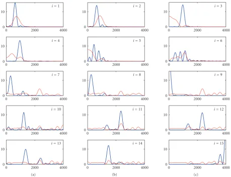
is a weighted sum (with weightsμi) ofk sig-nals obtained by passingsthrough the filter pairsziandJzi. As discussed inSection 9, the performance of the sub-space algorithms can be further studied by means of the FIR filters associated with the algorithms.Figure 9shows the fre-quency responses for the combined FIR filter pairs associ-ated with the SVD and ULV estimates inFigure 5. We used the low-rank ULV algorithmlulvfrom [47], which tends to
produce aV matrix whose leading columns are close to the principal right singular vectors. As expected, the SVD and ULV filters are therefore very similar in the frequency do-main.
The first two filters (fori = 1 and 2) are bandpass fil-ters that capture the largest formant at 700 Hz, while the next two filters (fori=3 and 4) are bandpass filters that capture the second largest formant at 1.1 kHz. The next six filters (for
i=5 through 10) capture more information in the frequency range 0–1500 Hz. The five filters fori=11 through 15 cap-ture the two formants at 2.3 kHz and 3.3 kHz. By adaptively placing bandpass filters at the portions of the signal with high energy, the subspace algorithms are able to extract the most important spectral components of the noisy signal, while at the same time, suppressing the noise in the frequency ranges with less energy.
9.3. GSVD/ULLV filters
The subspace algorithms for general noise have FIR filter in-terpretations similar to those for the white noise algorithms. To derive the FIR filters for the GSVD algorithms, let
ξ1,. . .,ξkdenote the firstkcolumns of the matrixΞ=X−T in (54), such that
Hgsvd=HYΦ=HΞ(:, 1 :k)ΦX(:, 1 :k)T. (80)
Then it follows fromSection 9.1that
s=AHY
Φ=D−1
k
i=1
φiHH(s)ξiJxi. (81)
We see that the coefficients of theith FIR filter pairξi and
Jxi consist of the elements of theith columns ofΞ = X−T andX(in reverse order), and the combined filters have co-efficients given by the convolution ofξiandJxi. In contrast to the SVD/UTV/VSV algorithms, these are not zero-phase filters.
In order to obtain bounds similar to (76), we make the reasonable assumption thatE2 ≤ H2. Then it follows from the definition of the GSVD that
Jxi
2=xi2≤ X2=
H E
2
≤2H2. (82)
From the definition, we also haveHξi2=γi. Following the same procedure as in the previous section, we thus obtain, fori=1,. . .,k,
HH(s)ξ
iJxi2≤2n1/2γiH2. (83) Similar to before, we thus include thekmost significant com-ponents in the signal, as determined by the filters defined by the vectorsξiandxi.
For the ULLV algorithm we insert the eigenvalue decom-position ofΨ(77) into (60) to obtain
Hullv=HVL−1
YMYT 0
0 0
LVT
=k
i=1
HVL−1y
iμiVLTyiT.