Supervised classification via constrained subspace and tensor sparse representation

BIROn - Birkbeck Institutional Research Online

Liao, L. and Maybank, Stephen and Zhang, Y. and Liu, X. (2017) Supervised

classification via constrained subspace and tensor sparse representation.

In: UNSPECIFIED (ed.) Neural Networks (IJCNN), 2017 International Joint

Conference on. IEEE Computer Society. ISBN 9781509061839.

Downloaded from:

Usage Guidelines:

Please refer to usage guidelines at

or alternatively

Supervised Classification via Constrained Subspace

and Tensor Sparse Representation

Liang Liao

1,2

, Stephen John Maybank

3

, Yanning Zhang

1

, Xin Liu

4

1

_{School of Computer Science, Northwestern Polytechnical University, Xi’an, P. R. China}

2

_{School of Electronics and Information, Zhongyuan University of Technology, Zhengzhou, P. R. China}

3

_{Birkbeck College, University of London, London, UK}

4

_{Information Center of Yellow River Conservancy Commission, Zhengzhou, P. R. China}

[email protected] (L. Liao), [email protected] (S. J. Maybank),

[email protected] (Y. Zhang), [email protected] (X. Liu),

Abstract—SRC, a supervised classifier via sparse representa-tion, has rapidly gained popularity in recent years and can be adapted to a wide range of applications based on the sparse solution of a linear system. First, we offer an intuitive geometric model called constrained subspace to explain the mechanism of SRC. The constrained subspace model connects the dots of NN, NFL, NS, NM. Then, inspired from the constrained subspace model, we extend SRC to its tensor-based variant, which takes as input samples of high-order tensors which are elements of an algebraic ring. A tensor sparse representation is used for query tensors. We verify in our experiments on several publicly available databases that the tensor-based SRC called tSRC outperforms traditional SRC in classification accuracy. Although demonstrated for image recognition, tSRC is easily adapted to other applications involving underdetermined linear systems.

I. INTRODUCTION

The concept of a data manifold plays an important role in a wide range of problems. Take image representation for example. An image of sizem×npixels with256gray-scales for each pixel has 256mn _{pixel configurations, but only a}

few correspond to particular classes of objects. Due to this redundancy in the raw representation of images, it is often assumed that that such as images belong to a manifold with a low intrinsic dimension (id). The intrinsic dimension is a measure of the number of degrees of freedom in the data [11], [14], [4]. The intrinsic dimension is the minimum number of parameters needed to describe the data structure such that the fundamental properties of the data are preserved. Briefly speaking, when data are represented by vectors in a high dimensional feature space, the manifold associated with the data is a nonlinear geometric structure which describes the distribution of the observed data and serves as a universal data set for the class in question [12].

A classifier called SRC (Sparse Representation Classifier) represents each query sample by a linear sum of a few highly associated training samples. In this way, SRC exploits the re-dundancy of the data and enjoys a high classification accuracy [19], [17]. Although first proposed for image classification, SRC can be easily adapted to a wide range of applications in which a sparse solution of an underdetermined linear model

is established [18], [5].

Later papers reinterpreted or challenged the mechanism of SRC [3], [13], [21], [20], [15]. For example, Zhang et al contend that collaboration offered by training samples of different classes contributes to the success of SRC. Shi et al propose a class-collaborative classifier called orthonormal`2 -norm algorithm to challenge the mechanism of SRC. Yang et al propose an affine sparse representation to improve SRC. Although these works have advanced our knowledge of SRC, a simple yet effective intuitive geometric model to interpret the mechanism of SRC is still unavailable.

We propose a geometric model called constrained subspace, which not only connects the dots of NN (Nearest Neighbor), NFL (Nearest Feature Line), NS (Nearest Subspace) and NM (Nearest Manifold) but also interprets SRC from the perspective of approximation by linear manifolds. Inspired by the recently reported technique called t-product [7], [1], [6], we extend SRC to its tensor-based variant while still retaining our constrained subspace model. We demonstrate in experiments that tSRC outperforms SRC and its non-tensor variant (Yang’s method) in classification accuracy.

The reminder of this paper is organized as follows. In Section II, the constrained subspace is introduced. Our tensor model built on a high-order algebraic ring and the tensor-based classifier tSRC are discussed in Section III. In Section IV, a sparse tensor solution of an underlying linear system is is obtained. The choice of features is discussed for tSRC. Section V presents experimental results obtained by applying the new classifier to publicly available databases. Section VI concludes this paper.

II. CONSTRAINED SUBSPACE

A. Notations and indexing

row. Similarly, we can concatenate a finite number of vec-tors/matrices together in one way or another as [A1,A2,· · ·] or [A1;A2;· · ·], as long as the sizes of the given entry vec-tors/matrices are compatible with each other. (iii) The values of the indices for tensors, including vectors and matrices, begin at0. For example,A(0,0)rather thanA(1,1)denotes the first scalar entry of matrix/tensor A. (iv) Colon notation: A(i,:)

denotes the i-th row of matrix/tensor A. A(:, j)denotes the

j-th column of matrix/tensor A. Note thatA(0,:)rather than

A(1,:) is the top row and A(:,0) rather than A(:,1) is the leftmost column.

B. Model

For the supervised classification problem, we first propose a geometric model called constrained subspace — Given

K classes and Ni training vectors of class i denoted by

x(1)_i ,x(2)_i , . . . ,x(Ni)

i , the constrained subspace Mi for class i is defined as a union of a set of of affine hulls as follows.

Mi =

(

Aiαi

αi ∈RNi

1Tαi = 1andkαk06κ6Ni

) (1)

whereAi .

=hx(1)_i ,x(2)_i , . . . ,x(Ni)

i

i

,1 denotes a vector with all its entries equal to1and the intrinsic dimension parameter

κis a positive integer.

Based on equation (1), we define a generalized classifier called NCSC (Nearest Constrained Subspace Classifier), which includes classifiers NN and NFL as low-dimensional special cases — Given a query vectorybelonging to one of the above mentioned K classes, NCSC classifiesyas follows.

class(y) = argminiminx∈Miky−xk2 (2)

C. Connecting the dots

Note that when κ= 1, Mi, as in equation (1), becomes a

set of feature points and NCSC, as in equation (2), becomes NN. When κ = 2, Mi becomes a set of feature lines and

NCSC becomes NFL [10]. Moreover, if the training samples are linearly independent, the intrinsic dimension ofMiis given

by

id(Mi) =κ−1. (3)

In other words, NN and NFL are just low-dimensional special cases of NCSC respectively with id= 0andid= 1. On the other hand, if constraints 1Tαi = 1 and kαk0 6

κ₆Ni are removed from equation (1), NCSC becomes NS

andMiis relaxed to a linear (unconstrained) subspaceSwith

id(S) = Ni. Since condition Mi ⊂ S is always satisfied

for all κ = 1,2,· · ·, Ni, we call our model the constrained

subspace model.

NCSC is also an approximation to the well-known classifier NM. Simply speaking, if the manifold assumption is true, manifold Mi serves as the universal sample set of class i.

Namely, given query sampleybelonging to one of the above mentioned K classes, NM employs a similar approach to equation (2), classifying yas follows.

class(y) = argminiminx∈Miky−xk2 (4)

By virtue of M1,· · ·,MK serving as universal sets of

samples, NM has a high classification accuracy. In order to improve NCSC’s accuracy, we contend that Mi should

be an accurate approximation to a manifold Mi for all i= 1,2,· · · , K.

Since the affine hull is also referred to as linear manifold, the essence of equation (1) is to use a union of a series of affine hulls withid=κ−1to approximate the corresponding manifold. Since Mi|κ=1 ⊂ Mi|κ=2 ⊂ · · · ⊂ Mi|κ=Ni, we

contend that in order to makeMia more accurate

approxima-tion toMi, one criterion is

id(Mi)uid(Mi). (5)

Equation (5) leads to the problem of estimating id(Mi)

from a finite number of observed samples. Although there are some interesting estimators available [4], [2], [9], their estimates vary with the choice of estimator and estimation parameters. A comprehensive evaluation of the estimators for a range of parameter values is still an open problem. The sparse representation employed by SRC offers an approach without the explicit estimation of intrinsic dimension.

SRC is class-collaborative while NCSC discussed in Section II-B is class-wise in the sense that, in SRC, training samples from different classes are allowed to represent a query sample but in NCSC, only training samples from a same class are used to represent a query sample.

It is easy to update NCSC from wise to class-collaborative. To obtain a class-collaborative version of NC-SC, construct a constrained subspace M to approximate to M=. S

iMiunder the criterionid(M)uid(M). Similar to equation (1),_Mis given by

M= (

Aα

α∈RN

1Tα= 1andkαk06κ6N )

(6)

where A = [. A1,A2,· · · ,AK], α .

= [α1;α2;· · ·;αK] and N =. P

iNi.

Given y, we seek a solution α∗ for y = Aα subject to

1Tα= 1 andkαk06κwhere κis a small positive integer satisfying κ u1 +id(M). Once α∗ is obtained, the class-collaborative NCSC classifiesy as follows.

class(y) = argmini∈{1,2,···,K}

y−Aλi(α∗) 2 (7)

whereλi :RN → RN is the characteristic function. λi(α∗)

returns a sparse vector of lengthN whose nonzero entries are the entries ofα∗associated with the training samples of class

i.

D. Yang’s method

To avoid an explicit estimation ofκfor NCSC, one can seek

α∗with the minimal`0-norm with the expectationkα∗k06κ. Namely,

α∗= argmin

α

Furthermore, one can solve the following `1-norm mini-mization problem rather than the NP-hard problem in equation (8).

α∗= argmin

α

kαk1 subject toy=Aαand1Tα= 1 (9) Equation (9) is Yang’s method [20], which imposes the constraint 1Tα= 1on SRC, in order to improve its classifi-cation performance. However Yang did not provide a concise geometric model to explain the essence of the constraint

1Tα = 1. From the perspective of manifold approximation, our constrained subspace model supports Yang’s method over SRC if the manifold assumption is true.

III. TENSORS

A. Definitions

In this section, we propose an tensor sparse representation for tensor data such as images (second-order tensors), which naturally come in the form of arrays rather than vectors. It is easy to extend the tensor sparse representation to high-order tensors, such as videos (third-order tensors). For presentation conciseness and without loss of generality we focus the discussion on second-order tensors such as images. First, we give some definitions as follows.

Definition 1. Tensor addition.Given tensorsAandBof size

m×n, the sumC =A+B is a new tensor of same size, satisfyingC(i, j) =A(i, j)+B(i, j)for alli= 0,1,· · ·, m−

1 andi= 0,1,· · · , n−1.

Definition 2. Tensor multiplication.Given tensorsAandB

of sizem×n, the productD=A◦Bis a new tensor of same size defined as the result of 2D circular convolution betweenA

andB, satisfyingD(i, j) =Pm−1

k1=0

Pn−1

k2=0A(k1, k2)B((i−

k1) modm,(j−k2) modn) for all i= 0,1,· · ·, m−1 and

j = 0,1,· · ·, n−1.

Given tensors A and B of the same size, the product C

can be computed efficiently by performing the 2D Fast Fourier Transform (2DFFT) and its inverse 2DFFT transform, because the following theorem holds.

Theorem 3. Fourier Transform. Given tensors A, B and the product D =A◦B, Dˆ(i, j) = ˆA(i, j) ˆB(i, j),∀ i and

j, where Dˆ,Aˆ and Bˆ are respectively the 2D Fast Fourier Transforms ofD,Aand B.

By Theorem 3, we haveA◦ B ≡B ◦ A.

Definition 4. Zero tensor. The zero tensor Z is defined by

Z(i, j) = 0for alliandj.

Definition 5. Identity tensor.The identity tensorEis defined by E(0,0) = 1andE(i, j) = 0for (i, j)6= (0,0).

It is not difficult to prove that the tensors of size m×n

defined above form an algebraic ringR. Furthermore, we also define a tensor vector/matrix as follows.

Definition 6. Tensor vector/matrix. Tensor vector/matrix is defined as vector/matrix whose atomic entries are tensors over

R rather than scalars over R. Operations between entries of tensor vector/matrix comply with the operations defined over R. Other manipulations of tensor vectors/matrices are analogous to these defined for vectors/matrices overR.

B. Connection to t-product.

The recently emerged t-product [7], [1], [6], [22], which is based on 1D circular convolution, can be described by our tensor model. Let’s take the t-product defined in [22] for example — Given tensors A and B of size m×n, if we leave A alone and constrain B satisfying B(i, j) ≡ 0

if i 6= 0, then C = A◦B, a tensor of size m×n, is equivalent to t-productC(t)=A(t)∗B(t)of sizem×1×n, where A(t) is a t-product tensor (we call tensors defined by t-product t-product tensors) of size m×1×n satisfying

A(t)(i,0, j) ≡ A(i, j) and B(t) is a t-product tensor of size 1 × 1 ×n satisfying B(t)(0,0, j) ≡ B(0, j) for all

i= 0,1,· · ·, mandj = 0,1,· · ·, n.C is equivalent toC(t)

in the sense that C(i, j)≡C(t)(i,0, j)for alliandj. Since our approach defined in Section III-A manipulates tensors from multiple directions, (i.e., row and column direc-tions for second-order tensors) while t-product manipulates tensor only from one direction, our tensor model is more generalized.

C. Tensor sparse representation and tSRC

Given training tensors X1,X2,· · · ,XN belonging to K

classes, a query tensorY can be represented by a sparse linear sum of the training tensors as follows.

Y =

N

X

k=1

βk◦Xk subject to N

X

k=1

βk=E (10)

On defining the column vector β= [. β1;β2;· · ·;βN] and

the row vectorA= [. X1,X2,· · · ,XN], equation (10) can be

rewritten in its tensor vector/matrix form. A sparse solution

β∗ _{is given by the following `}

1-norm minimization.

β∗= argminβ β

1 subject to Y =A◦βand PN

k=1βk =E

(11)

whereβ 1

. =

N

P

k=1

m−1

P

i=0

n−1

P

j=0

βk(i, j)

.

We define the `2-norm of a second-order tensor X by

kXk₂ =. qP

i

P

j|X(i, j)|

2

. Then, we propose a tensor based classifier called tSRC in Algorithm 1.

Algorithm 1 tSRC — tensor SRC on algebraic ringR Input: Query tensor Y and training tensors X1, X2, · · ·,

XN of K classes.

Output: Class label ofY.

1: Calculate β∗= [. β₁∗;· · · ;β_N∗] as in equation (11); 2: ri← kY −Aδi(β∗)k2 ∀i= 1,2,· · ·, K ; 3: return class(Y)←argmini∈{1,2,···,K}ri ;

In Algorithm 1, δi : RN → RN is the characteristic

whose nonzero entries are the coefficient tensors associated with the training tensors of classi. On denoting the index set of the training tensors of classibySiand definingδNj ∈R

N

as the sparse column tensor vector with entry j equal to E

and all other entries equal to Z,δi(β)is defined as follows. δi(β) =

X

j∈Si

diag δ_NjβT

(12)

IV. `1-NORM MINIMIZER AND FEATURE EXTRACTION

A. Minimizer

We give a solver for equation 10, which recasts the tensor-based optimization problem as a traditional`1-norm optimiza-tion problem as follows.

First, we give the following notations — given a tensor

X of size m×n and integers km, kn, X(km,kn) denotes a

tensor of the same size, satisfying X(km,kn)_{(i, j) =X((i−}

km) modm,(j−kn) modn), for alli= 0,1,· · · , m−1and j = 0,1,· · ·, n−1. We denote the vector versions ofX and

X(km,kn) _{respectively byxandx}(km,kn)_.

Then, equation (11) can be transformed into the form of equation (9) — given training tensors X1,X2,· · ·,XN of

size m×n, the columns ofAin equation (9) are given by

A(:,(k−1)mn+kmn+kn) =x(_kkm,kn) (13)

wherex(km,kn)

k is the vector version of X

(km,kn)

k for allk=

1,2,· · ·, N,km= 0,1, . . . , m−1andkn= 0,1, . . . , n−1.

Furthermore, settingyas the vector version ofY and with the original constraint 1Tα= 1 replaced by

N

P

k=1

α((k−1)mn+kmn+kn) =E(km, kn) ∀km= 0,1,· · · , m−1and

∀kn = 0,1,· · ·, n−1

(14)

α∗obtained as in equation (9) is equivalent toβ∗ obtained as in equation (11).

Since A(:,(k − 1)mn + kmn + kn) corresponds to

βk(km, kn), the tensor vectorβ∗ .

= [β₁∗;β₂∗;· · · ;β_N∗] can be easily restored by

β_k∗(km, kn) =α∗((k−1)mn+kmn+kn) (15)

Equations (13) and (15) reveal that tSRC is an extension of SRC (more accurately Yang’s method) which enlarges the original training volume by extending a single sample Xk to

multiple samples X(km,kn)

k for allkm= 0,1,· · ·, m−1and kn = 0,1,· · ·, n−1.

B. Feature extraction

There exist a wide range of popular and effective feature ex-tractors, such as PCA (Principle Component Analysis), which extract features as vectors rather than tensors. To work with these feature vector extractors, one can extract a collection of feature vectors from a set

X(km,kn)

∀km, kn rather than

just one feature vector from one sample X.

With the minimizer discussed in Section IV-A, which flat-tens flat-tensors to vectors, tSRC can conveniently handle feature

vectors. More specifically, tSRC uses the following equation to work with feature vectors.

A(:,(k−1)mn+kmn+kn) = ˆx(kkm,kn) (16)

where xˆ(km,kn)

k denotes the feature vector extracted from

X(km,kn)

k .

V. EXPERIMENTS

A. Settings

Although tSRC and SRC-like classifiers can be used for purposes including but not limited to supervised classifica-tion, in this secclassifica-tion, we evaluate tSRC for supervised image classification on several publicly available databases.

In order to get statistically stable classification accuracies by classifying a sufficient number of query samples for each training set, our experiments contain multiple rounds of classification. In order to avoid unnecessary perturbation-s of claperturbation-sperturbation-sification accuracy, in each round, query perturbation-sampleperturbation-s and training samples are randomly chosen and then kept unchanged in the evaluation of the relevant classifiers. After all rounds, the classification accuracy of each classifier is given byaccuracy=w/W wherewis the total number of correctly classified query samples andW is the total number of query samples from all rounds.

B. Evaluations on the raw MNIST data

In this section, we apply the relevant classifiers to the raw MNIST database [8]. The MNIST database of handwritten digits contains a large number of image samples of size

28×28 pixels belonging to 10 classes. There are 60,000

training images (roughly6,000images per class) and10,000

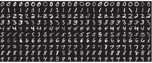
[image:5.612.316.561.472.574.2]

query images (roughly1,000images per class) in the MNIST database. Figure 1 shows some examples of the MNIST database.

Fig. 1. Some image samples of the MNIST database.

Due to its large number of samples, small image size and unvarying illumination condition, it is ideal to evaluate the manifold assumption, constrained subspace model and the relevant classifiers.

(9). To construct the underdetermined linear system in equa-tion (9), the column number ofA should be larger than784. We observe the classification performance when the number of training samples is changed. Thus, in each classification round, we set the number of training samples of class irespectively by Ni = 100, 150, 200, 250, 300 and 350. The experiment

contains10classification rounds. In each round,1,000query images (100 images/class×10 classes) are randomly chosen from the MNIST test set andN training samples (N samples = Ni samples/class ×10 classes) are randomly chosen from

the MNIST training set.

To evaluate the efficacy of the t-product [7], [1], [6], our tSRC is developed as two variants, tSRC-1D and tSRC-2D. Classifier tSRC-1D is tSRC via tensor sparse representation offered by the t-product, but with the constraint that the only non-zero scalar entries of tensor βk are in βk(0,:) for all k = 1,2,· · ·, N. More specifically, in the t-product model, tensor Xk of size m×n is recast to t-product tensor X_k(t)

of size m×1×n, tensor βk is recast to t-product tensor

β_k(t) of size1×1×n, satisfying,∀ i= 0,1,· · ·, m−1and

j = 0,1,· · ·, n−1

(

X_k(t)(i,0, j) =Xk(i, j)

β_k(t)(0,0, j) =βk(0, j)

. (17)

Thus,C=. Xk◦βk is equivalent toC(t) .

=X_k(t)∗β(_kt)in the sense that C(i, j)≡C(t)(i,0, j).

In tSRC-2D, the constraint imposed on the nonzero entries inβk found in tSRC-1D is removed. In comparison with SRC

and Yang’s method, the computational complexity of solving the linear system in tSRC is dramatically increased primarily because tensors are employed.

In order to obtain results of tSRC in a reasonable time, the computational complexity of tSRC is reduced. We constrain tSRC-2D by setting βk(i, j) equal to zero outside the set of

values defined byi∈ {(m−1),0,1}andj∈ {(n−1),0,1}. Similarly, we constrain tSRC-1D by setting βk(i, j) equal

to zero outside the set of values defined by i = 0 and

j ∈ {(n−1),0,1}. These constraints on 1D and tSRC-2D are also kept unchanged in the experiments on other databases.

This constraint imposed on tSRC exploits the fact that in a small neighborhood of an image, the grayscales of the pixels are highly correlated.

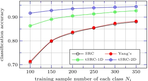
Figure 2 shows the classification accuracy curves of the relevant classifiers SRC, Yang’s, tSRC-1D and tSRC-2D on the raw MNIST data.

Several observations are made on Figure 2.

(i) As Ni increases, the classification accuracy increases.

Since the constrained subspace is a linear approximation to manifold of low intrinsic dimension, with Ni increasing, we

contend that the approximation to the underlying manifold becomes more accurate and leads to a higher classification accuracy.

(ii) The second observation is that the classification accuracy of Yang’s method is higher than that of SRC, albeit marginally.

100 150 200 250 300 350 0.70

0.80 0.90

training sample number of each classNi

classification

accuracy

SRC Yang’s

[image:6.612.318.557.58.188.2]

tSRC-1D tSRC-2D

Fig. 2. Accuracy curves with an increasing number of training samples obtained by SRC, Yang’s method, tSRC-1D and tSRC-2D on the raw MNIST data.

This versifies the report by Yang [20] and supports the manifold assumption and our constrained subspace model.

(iii) The classification accuracy of tSRC is higher than those of SRC and Yang’s method.

(iv) The accuracy of 2D is higher than that of tSRC-1D. We contend that this is because tSRC-2D exploits more image structure information both in the row direction and the column direction while tSRC-1D only exploits structure information in the column direction.

C. Evaluations with feature extraction

Since tSRC (tSRC-1D and tSRC-1D) can be transformed to its flattened version involving vectors, we are particularly inter-ested in classification accuracies obtained on feature vectors. Given the effectiveness and popularity of PCA in data analysis, we evaluate SRC, Yang’s method, tSRC with PCA features. For tSRC, given tensorX(km,kn)

k and after vectorizing it, we

extract its PCA feature vectorxˆ(km,kn)

k as in equation (16).

1) MNIST data: Figure 3 gives the classification accuracy curves of SRC, Yang’s method and tSRC by repeating the experiment in Section V-B but with the PCA feature extractor. The feature dimension isd= 100.

Compared to the classification results shown in Figure 2, the accuracies obtained with PCA are significantly increased. The observations drawn from Figure 2 also apply to Figure 3. 2) ORL data: We are also interested in classification ac-curacies on image datasets with a larger image size but with a smaller number of images. The ORL database is one such database. The ORL database contains 400 facial images (10

images/class × 40 classes) of size 112 × 92 pixels, taken at different times with variations of facial expressions, details and poses etc.

Figure 4 shows the images from a sample subject (class) of the ORL data.

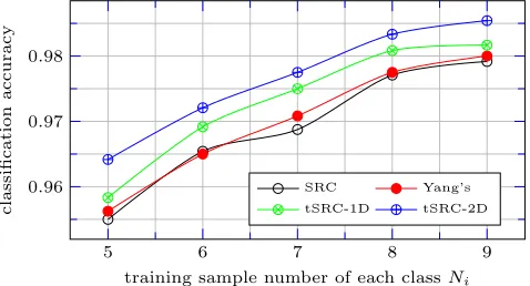
Figure 5 gives the accuracy curves of SRC, Yang’s method and tSRC on this database.

In our experiments, the number of training samples for each class is respectively taken asNi= 5,6,7,8,9. For each value

ofNi, the accuracy of each classifier is obtained from multiple

100 150 200 250 300 350 0.92

0.94 0.96

training sample number of each classNi

classification

accuracy

SRC Yang’s

[image:7.612.54.294.58.189.2]

tSRC-1D tSRC-2D

[image:7.612.317.562.138.217.2]

Fig. 3. Accuracy curves with an increasing number of training samples obtained by SRC, Yang’s method, tSRC-1D and tSRC-2D on the PCA features of the MNIST data.

Fig. 4. Images of a sample subject (class) of the ORL data.

classes are randomly chosen as the training samples. The re-maining samples are taken as the query samples. Thus, in each classification round, the number of query samples is(10−Ni)

samples/class ×40 classes. Both training samples and query samples are extracted by PCA to yield100-dimensional feature vectors.

In order to have the same number of query samples in multiple rounds for each value of Ni, corresponding toNi=

5,6,7,8,9, the number of classification rounds is respectively set as 12,15,20,30,60. In other words, each accuracy point in Figure 5 is the result of classifying 2400 random query samples.

The observations on the curves in Figure 4 are the same as the observations drawn in Section V-B on the raw MNIST data .

3) Extended Yale B data: We aslo evaluate the classifiers on the Extended Yale B database [16]. The Extended Yale B database contains 2,414 cropped frontal face images of

5 6 7 8 9

0.96 0.97 0.98

training sample number of each classNi

classification

accuracy

SRC Yang’s

tSRC-1D tSRC-2D

Fig. 5. Accuracy curves with an increasing number of training samples ob-tained by SRC, Yang’s method, tSRC-1D and tSRC-2D on features extracted by PCA on the ORL data.

size 192×168 pixels from 38 subjects (classes), roughly 64

image per class. The images from this database are taken under vaying illumination.

[image:7.612.51.300.240.273.2]

Figure 6 shows some samples of the Extended Yale B database. It is clear that the average grayscales of the samples even in the same class are perceivably different.

Fig. 6. Image samples of the Extended Yale B database under varying illumination condition.

Since the effect of the illumination can be modeled by a scale factor, it is believed that varying illumination tends to reduce the accuracy of the approximation to the data by the underlying constrained subspace. This might challenge the effectiveness of the affine linear representation offered by the constrained subspace model.

To reduce the influence of varying illumination, we first en-hance the grayscale contrast of images by means of grayscale histogram equalization. Then, we extract the PCA features of the enhanced images with feature dimension d = 100. There are 10 classification rounds for each value of Ni, .

In each round, 912 images (912 images = 24 images/class × 38 classes) are randomly chosen as query samples. N

training samples (where N samples =Ni samples/classes×

38classes) are randomly chosen from the rest of the samples respectively with Ni = 16,20,24 and28.

Figure 7 shows the accuracy curves, with an increasing number of training samples, for SRC, Yang’s method, tSRC-1D and tSRC-tSRC-1D. Each point on the curves is the accuracy of classifying9,120random query images (9,120images= 912

images/round ×10 rounds).

16 18 20 22 24 26 28

0.94 0.96 0.98

training sample number of each classNi

classification

accuracy

SRC Yang’s

tSRC-1D tSRC-2D

Fig. 7. Accuracy curves with an increasing number of training samples obtained by SRC, Yang’s method, tSRC-1D and tSRC-2D on the PCA features of the Extended Yale B data.

[image:7.612.319.556.523.651.2] [image:7.612.55.294.554.683.2]

of tSRC (tSRC-1D and tSRC-2D) is higher than those of SRC and Yang’s method.

However, compared to the results shown in Figures 2, 3, and 5, the accuracy differences between SRC, Yang’s and tSRC are less predominant although image enhancement and PCA feature extraction have been used.

Although our present work only focuses on evaluations and comparisons of the performances of relevant classifiers, we argue that, to enlarge the classification difference of tSRC and its non-tensor counterparts, besides more sophisticated image enhancement and feature extraction techniques, a reduced region of the entries constrained to zero in βk for all k

(discussed in Section V-B) might be helpful, but at the cost of a significant increase of computational complexity. Our present experiments clearly show the differences in the classification accuracies of SRC, Yang’s method and tSRC.

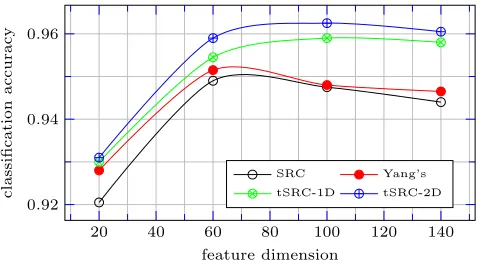
4) Evaluations with increasing feature dimension: In the experiments in this section, the training samples are fixed but feature dimension is changed. The experiment is on the PCA feature vectors extracted from the ORL database. The feature dimension is respectively set by d = 20, 60, 100

[image:8.612.54.294.434.566.2]

and 140. In each classification round, 200 training samples (5 samples/class × 40 classes) are randomly chosen. The remaining200samples (also5samples/class×40classes) are taken as the query samples. There are10classification rounds. In other words, each point in Figure 8 is the accuracy of classifying2,000samples (200samples/round ×10 rounds). Figure 8 gives the accuracy curves over different values of feature dimension. The curves shown in Figure 8 verify the accuracy of tSRC over its non-tensor counterparts.

20 40 60 80 100 120 140 0.92

0.94 0.96

feature dimension

classification

accuracy

SRC Yang’s

tSRC-1D tSRC-2D

Fig. 8. Accuracy curves with an increasing feature dimension obtained by SRC, Yang’s method, tSRC-1D and tSRC-2D on the PCA features of the ORL data.

Another interesting observation found from Figure 8 is that the increase in feature dimension does not always lead to an increase in the classification accuracies of SRC, Yang’s method and tSRC. When feature dimension d is very small (for example, in Figure 8, when feature dimension d <60), an increase of d does increase classification accuracy since more useful information in the data is exploited. When d

is relatively high (for example when d > 100 in Figure 8), the features contain over-detailed information from the

data which can cause the classification accuracy to decline. Similar results are obtained in classifying samples from other databases. The results are not reported here in order to reduce the length of the paper. However, we would like to add another interpretation to this observation from the perspective of constrained subspace — Each classifier in our experiments requires the training samples to be over-complete in order to construct an underdetermined linear system y = Aα, which has a low-rank matrix A. The over-completeness of training samples is highly associated with feature dimension

d. When the number of training samples is fixed, an increase of d of a query sample usually make it less likely that the given training samples will be complete for the query sample. When d increases, in order to find a constrained space M to include the query sample, the intrinsic dimension id(M) must increase. In other words, the solution α∗ of equation (11) or β∗ _{of equation (8) becomes less sparse. We call this}

phenomenon the “inflation of the constrained subspace”. The inflated constrained subspace with id(M) much larger than that of the manifold is a less accurate linear approximation to the underlying manifold and therefore causes a reduction in the accuracy of the classification.

VI. CONCLUSIONS

A constrained subspace model is proposed for a tensor-based classifier called tSRC. In this model, the constrained subspace is defined as a union of a series of affine hulls. Each affine hull is spanned by training samples via sparse representation, and serves as a local linear approximation of the corresponding manifold.

This model establishes a generalized framework for some classical classifiers including NM, NN, NFL and NS. In this model, NN, NFL and NS are all approximations to NM, which in principle enjoys a high classification accuracy. The constrained subspaces of NN and NFL have respectively intrinsic dimensions0 and1.

To make the constrained subspace a more accurate approxi-mation to the corresponding manifold, we contend that the in-trinsic dimension of the constrained subspace should be equal to that of manifold. Based on this assumption, we contend that the sparsity parameterκof the sparse representation, employed with the training samples to span the constrained subspace, should be carefully tuned. Thus, the searching of the nearest constrained subspace point to a query data point is formulated as a constrained least-squares problem.

To circumvent the explicit intrinsic dimension estimation and exploit the collaboration offered by different classes, the constrained subspace model helps transform the least-squares problem to a spare representation problem via`1-norm optimization.

Thus, the proposed constrained subspace model not only connects the dots of NN, NFL, NS, SRC and NM but also offers an intuitive explanation to the mechanism of SRC and Yang’s method which is a variant of SRC.

tensors is defined via high-order circular convolution. Then we propose a novel classifier called tSRC. The pro-posed classifier is a tensor variant of SRC subject to the conditions inspired from the constrained subspace model.

Our experiments on several publicly available databases verify our claims on the constrained subspace model and tSRC. The proposed tSRC is scalable in its computational complexity control. At the cost of a manageable complexity increase, tSRC is more accurate than competing classifiers.

ACKNOWLEDGMENT

The authors would like to thank the anonymous reviewers for their valuable suggestions.

REFERENCES

[1] K. Braman, “Third-order tensors as linear operators on a space of matrices,” Linear Algebra and its Applications, vol. 433, no. 7, pp. 1241–1253, 2010.

[2] F. Camastra and A. Vinciarelli, “Estimating the intrinsic dimension of data with a fractal-based method,” IEEE Transactions on Pattern Analysis and Machine Intelligence, vol. 24, no. 10, pp. 1404–1407, 2002. [3] M. Elad, M. A. Figueiredo, and Y. Ma, “On the role of sparse and redundant representations in image processing,” inProceedings of the IEEE, vol. 98. IEEE, 2010, pp. 972–982.

[4] M. Fan, H. Qiao, and B. Zhang, “Intrinsic dimension estimation of manifolds by incising balls,”Pattern Recognition, vol. 42, no. 5, pp. 780–787, 2009.

[5] X. Huang, D. P. Dione, C. B. Compas, X. Papademetris, B. A. Lin, A. Bregasi, A. J. Sinusas, L. H. Staib, and J. S. Duncan, “Contour tracking in echocardiographic sequences via sparse representation and dictionary learning,”Medical image analysis, vol. 18, no. 2, pp. 253– 271, 2014.

[6] M. E. Kilmer, K. Braman, N. Hao, and R. C. Hoover, “Third-order tensors as operators on matrices: A theoretical and computational framework with applications in imaging,” SIAM Journal on Matrix Analysis and Applications, vol. 34, no. 1, pp. 148–172, 2013. [7] M. E. Kilmer and C. D. Martin, “Factorization strategies for third-order

tensors,”Linear Algebra and its Applications, vol. 435, no. 3, pp. 641– 658, 2011.

[8] Y. LeCun and C. Cortes, “The MNIST database of handwritten digits,” http://yann.lecun.com/exdb/mnist/.

[9] E. Levina and P. J. Bickel, “Maximum likelihood estimation of intrinsic dimension,” inAdvances in Neural Information Processing Systems 17, L. K. Saul, Y. Weiss, and l. Bottou, Eds., Cambridge, MA, December 2005, pp. 777–784.

[10] S. Z. Li and J. Lu, “Face recognition using the nearest feature line method,” IEEE Transactions on Neural Networks, vol. 10, no. 2, pp. 439–443, 1999.

[11] S. Z. Li and A. K. Jain,Handbook of Face Recognition. Springer, 2005, ch. Introduction, pp. 141–142.

[12] L. Liao, Y. Zhang, S. J. Maybank, and Z. Liu, “Intrinsic dimension esti-mation via nearest constrained subspace classifier,”Pattern Recognition, vol. 47, no. 3, p. 1485, 1485–1493 2014.

[13] G. Liu, Z. Lin, S. Yan, J. Sun, Y. Yu, and Y. Ma, “Robust recovery of subspace structures by low-rank representation,”IEEE Transactions on Pattern Analysis and Machine Intelligence, vol. 35, no. 1, pp. 171–184, 2013.

[14] G. Peyr´e, “Manifold models for signals and images,”Computer Vision and Image Understanding, vol. 113, no. 2, pp. 249–260, 2009. [15] Q. Shi, A. Eriksson, A. van den Hengel, and C. Shen, “Is face

recogni-tion really a compressive sensing problem?” in2011 IEEE Conference on Computer Vision and Pattern Recognition (CVPR), June 2011, pp. 553–560.

[16] UCSD, “Extended Yale face database B,” http://vision.ucsd.edu/extyaleb/CroppedYaleBZip/CroppedYale.zip. [17] A. Wagner, J. Wright, A. Ganesh, Z. Zhou, H. Mobahi, and Y. Ma,

“Toward a practical face recognition system: Robust alignment and illumination by sparse representation,” IEEE Transactions on Pattern Analysis and Machine Intelligence, vol. 34, no. 2, pp. 372–386, 2012. [18] L. Wang, F. Shi, Y. Gao, G. Li, J. H. Gilmore, W. Lin, and D. Shen,

“Integration of sparse multi-modality representation and anatomical con-straint for isointense infant brain mr image segmentation,”NeuroImage, vol. 89, pp. 152–164, 2014.

[19] J. Wright, A. Y. Yang, A. Ganesh, S. S. Sastry, and Y. Ma, “Robust face recognition via sparse representation,” IEEE Transactions on Pattern Analysis and Machine Intelligence, vol. 31, no. 2, pp. 210–227, 2009. [20] J. Yang, L. Zhang, Y. Xu, and J.-y. Yang, “Beyond sparsity: The role

of`1-optimizer in pattern classification,”Pattern Recognition, vol. 45,

no. 3, pp. 1104–1118, 2012.

[21] D. Zhang, M. Yang, and X. Feng, “Sparse representation or collaborative representation: Which helps face recognition?” in2011 IEEE Interna-tional Conference on Computer Vision (ICCV), 2011, pp. 471–478. [22] Z. Zhang, G. Ely, S. Aeron, N. Hao, and M. Kilmer, “Novel methods

for multilinear data completion and de-noising based on tensor-svd,” in