1.0 INTRODUCTION
Headphone modelling concerns the solution of a number of coupled problems centring on a small mechanical diaphragm vibrating in an enclosed space. Frequently, the electro-acoustic transduction mechanism is dynamic, and the transfer functions between electrical (v,i) and mechanical (F,u) quantities must be considered. These transfer functions will in part depend on the acoustic load (p,U) acting on the diaphragm, and this acoustic load will also determine the pressure radiated by the diaphragm which will, via a transfer function dependant on the type of enclosure and the physiology of the wearer, eventually impinge on the tympanic membrane.
Whatever solution method is attempted, it is probable that the end-user will regard the device as one which generates acoustics pressures in response to the application of electrical voltages. It seems sensible therefore to commence the analysis by working towards an evaluation of a transfer function in terms of
(1)
To this end, the technique of lumped element modelling is introduced below.
2.0 LUMPED ELEMENT MODELING
A great many authors have used lumped-element (or analogue circuit) modelling as a way of reducing the differential equations of motion which describe
coupled electro-mechano-acoustic systems into familiar networks of electrical components [eg 1,2,3]. The method has the advantage that fully coupled models may be constructed rapidly, and for those familiar with electrical networks and filters, the analysis of the resulting circuit analogues is straightforward and intuitive.
The most substantial disadvantage of lumped element models is that in order to be ‘lumped’, each element must not in itself exhibit wave behaviour. To clarify with a mechanical example – if a vibrating diaphragm is to be considered as a lumped mass, then all points on that diaphragm must oscillate with identical velocity (in magnitude and phase). Since most mechanical and acoustic systems behave modally (in a distributed rather than lumped fashion) within the audio bandwidth, some might consider the technique to be of limited utility, perhaps restricted to low-frequency analysis. However, headphones are small devices, and this allows the use of the technique to illustrate the fundamental behaviours of the system across a useful range of frequencies.
2.1 Simple driver / ear canal model
In order to illustrate generic headphone design constraints, the selection of a dynamic transducer will apply to most practical applications and facilitate simple electro-mechanical modelling of the system. Following conventional analysis the acoustic (p,U) impedance analogue for a dynamic driver is as shown in Figure 1.
AUDIO AT HOME – AES 21ST UK CONFERENCE 2006
1
M.R.AVIS and L.J.KELLY
([email protected])
([email protected])
Acoustics Research Centre, Research Institute for the Built and Human Environment,
University of Salford, UK
M.R AVIS AND L. J.KELLY
All except ZABand ZAFare determined by the selection
of the drive unit, and these parameters (small-signal or Thiele-Small) may be extracted using conventional measurement techniques. By contrast the acoustic loads are determined by the nature of the enclosure.
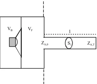
The simplest design case we might consider concerns a driver in a sealed enclosure, attached rigidly to the side of the head (Figure 2). The acoustic load will be partially dependent on the input impedance to the ear canal Za,0 which is itself a function of canal length,
cross-section and termination impedance. Despite publications suggesting that the canal is in fact roughly conical, the simplest model assumes a rigid
cylinder terminated with known impedance [4], in which case [5]:
(2)
The lumped impedance of an enclosed
volume is well-known:
2 0
0
c
V
P
V
C
A
(3)Therefore the acoustic loads ZAB and ZAF shown in
Figure 1 can be replaced by the network shown in Figure 3 below:
AUDIO AT HOME – AES 21ST UK CONFERENCE 2006
2
Figure 1: Acoustic impedance analogue of generic dynamic driver where:
e = applied voltage Bl = force factor (NA-1)
SD = diaphragm area (m2)
RE = d.c. coil resistance (Ω)
LE = coil inductance (H)MAD = moving diaphragm mass, acoustic units (kgm-4)
CAD = suspension compliance, acoustic units (m5N-1)
RAD = suspension resistance, acoustic units (Nsm-5)
ZAB = acoustic backload (Pa.sm-3)
ZAF = acoustic frontload (Pa.sm-3)
1/{jω(LESD2/(Bl)2}
eBl/{SD(RE+jωLE)}
ZAF RAD
(Bl)2/{R
ESD2} MAD
U ZAB
CAD
VB VF
ZA,0 S1 ZA,T
l
Figure 2: Simple model of headphone / ear system
Figure 3: Acoustic circuit analogue for simple model of headphone / ear system
C
ABC
AFZ
A,0U
The pressure at the input to the ear canal P0 is (of
course) a function of driver velocity, which itself takes a second-order bandpass response around a resonant frequency determined by diaphragm mass MAD and the series combination of suspension and
backload compliances CAD CAB / { CAD+CAB }.
However, VFgenerates a shunt compliance which
low-pass filters this pressure, suggesting this volume should be kept as small as practicable whilst comfortably accommodating the pinnae of users. P0 describes the pressure at the input to the ear canal,
whilst the subjective sensation of music listening is clearly dependant on the pressure at the tympanum. Relating the pressures at each end of a cylindrical duct of known termination impedance:
(4)
This implies that there is a modal relation between the
pressures at each end of the ear canal, which further modifies the input acoustics pressure (itself a function of the modal ear canal input impedance).
2.2 Leak behaviour
Our assumption that the headphone will be rigidly attached to the side of the head is clearly erroneous; in most circum-aural designs the cup will be equipped with cushions which are held against the side of the head by headband tension. We might imagine that in certain circumstances the seal with the head would be imperfect, leading to leaks, as illustrated in Figure 6. Figure 4 shows the transfer function p0 /e for two
cases – the load is assumed to be purely compliant in case (2), and purely the input impedance to the ear canal (no coupler volume) in case (1). The latter case clearly shows the influence of ear canal resonances, whereas the former (also shown by Poldy [3]) over predicts the low frequency sensitivity. In both cases the chosen driver parameters give a driver resonance at about 1.5 kHz.
In Figure 5, the effect of the parallel impedances of ear canal and shunting coupler volume can be seen, for three values of VF. This time the magnitude
response is that of the pressure at the ear drum as a function of drive unit input voltage. As expected, a large coupler volume reduces sensitivity, although it could be argued that increased sensitivity for small couplers comes at the cost of narrow bandwidth of reproduction.
AUDIO AT HOME – AES 21ST UK CONFERENCE 2006
3 Figure 5: | p1 /e | for three values of VF
Figure 4: | p0 /e | for (1): finite ear canal input
impedance, VF =0 and (2): VF =5cc, infinite ear
canal input impedance
Figure 6: Simple model of headphone / ear system including leaks
VB VF
ZA,0 S1 ZA,T l
M.R AVIS AND L. J.KELLY
Such leaks may be modelled most simply as a branch pipe which further diverts driver volume velocity from the driver. Therefore the acoustic load becomes that shown in Figure 7. Small leaks will almost certainly exhibit lossy as well as inductively reactive behaviour, but as a first approximation the leak may be modelled as a lumped mass:
Incorporated into the analogous circuit in Figure 7, this impedance acts as a high-pass filter (Figure 8). This behaviour seems intuitively correct, when one considers the spectral effect of pushing the cup more firmly to the side of the head. The model also agrees tolerably with headphone measurements on an artificial head incorporating prefabricated leak ‘tubes’, and with measurements on human users of various head size and pinna-jaw configuration.
A first refinement of this model would place a resistive loss in series with MAL , but as is often the
case with damping materials the precise determination of acoustic resistance is difficult and may be best approached by attempting to fit measured data with the model approximation. Additionally, Poldy [3] presents a number of formulae for holes and slits which give suggested values for reactive and resistive lumped components as functions of frequency, which this author has used with mixed results.
2.3 Closed vs. open back designs
As has been shown in section 2.3, leak impedances can significantly change the pressure response at the users ear drum. Unfortunately the filtering effect imposed by leaks cannot be compensated electronically, since the spectral modifications are highly variable between users. What is required is a method by which inter-user leak variability is lessened
in its effect on the spectrum at the ear drum. This is usually accomplished by instituting a large, predetermined ‘leak’ between VF and VB and / or free
space. A simple configuration is shown in Figure 9. As long as the (fixed, pre-determined) front / back leakage path has small impedance compared to the variable leaks around the cushion, the spectrum at the ear drum can be maintained considerably more constant between users than might otherwise be the case. The analogue circuit now takes the form shown in Figure 10.
Unfortunately, at the same time the sensitivity of the device is reduced considerably. In many circumstances, such a loss in sensitivity is tolerable since as long as the drive unit remains linear in operation to a sufficiently large excursion, the drop in sound pressure level at the ear may be compensated by increasing the magnitude of the electrical input accordingly.
If, as in Figure 11, the open-back design lacks low-frequency emphasis, this may be applied electronically. The key feature of using a large, fixed, resistive ‘leak’ (i.e. an open-back configuration) is that in comparison with Figure 8, leak cases (1) to (3) have a far less significant effect on the pressure at the ear.
AUDIO AT HOME – AES 21ST UK CONFERENCE 2006 (5)
4
Figure 7: Acoustic circuit analogue for simple model of headphone / ear system including leaks
C
ABC
AFZ
A,0U
P
0M
ALVB
VF
ZA,0 S1 ZA,T
l
S2
l2
Figure 8: | p1 /e | for three leak conditions of increasing sizeFigure 9: Acoustic circuit analogue for open-back
An additional potential difficulty is found in the loss of passive attenuation through the cup when using an open-back approach. Where listening is to take place in a noisy environment (for instance cueing in ‘live’ sound reproduction events, outside broadcasts, or for some telephony / radio communication applications) then the open back solution is often made impracticable by noise masking of the signal. In such situations, the headphone has to act simultaneously as hearing protector and communication device; some of the issues surrounding the design of successful hearing protectors are considered in section 2.4.
2.4 Headphones as hearing protectors Propagation from free space to beneath the cup can take place via two mechanisms; leaks between cushions and head, and by structure-borne transmission through the cup itself. Rather than exciting the cup into bending-wave motion, it is much more likely that the cup itself remains stiff and executes whole-body motion on the ‘suspension’ provided by the cushions. The mode of this oscillation has a significant impact on sound propagation. Where the cup ‘rocks’ (the cushion, on opposite sides of the ear, executing out-of-phase motion) then the space under the cup is not compressed, and structure-borne transmission is insignificant. However if the cup executes single-plane motion normal to the side of the head (sometimes called the ‘breathing mode’) then the compliant volume of air beneath executes significant compression and rarefaction, generating acoustic pressures.
The cup (if it executes whole-body motion) may simply be regarded as a mass, and the cushion as a suspension providing compliance and damping. In addition, some authors consider separately the
compliance and damping offered by the flesh between the cushion and the skull. The circuit analogue then takes the form shown in Figure 12.
Transfer function P1(jω)/P0(jω) describes the
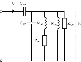
attenuation of the hearing protector. Neglecting for a moment the leak impedances, we can see that the system will be resonant, with the mass of the cup bouncing on the compliance provided by the air volume, with some damping afforded by the cushion and flesh. The circuit may be solved to give a detailed description of the separate effects of cushion and flesh compliance and damping (schroter), or alternatively for a more rapid and intuitive description
these terms may be considered as a single lumped compliance and resistance CA1 and RA1 . Then:
1 1
2 0
1
) ( 1
1
A AF A
AF Acup
AF j C R
C C M
C j P
P
(6)
AUDIO AT HOME – AES 21ST UK CONFERENCE 2006
5 Figure 10: Acoustic circuit analogue for open-back headphone / ear system including leaks
Figure 11: (a) - Closed back response, no leaks; (b) – open back response, no leaks and leak case (1); (c) – open back response, leak case (2); (d) – open back response, leak case (3)
CAF MA1 MAL ZA,0 P0
RA1
Figure 12: Acoustic circuit analogue for open-back headphone / ear system including leaks
MA,leak RA,leak
MA,cup
CA,flesh
RA,cush
P0
RA,flesh
CAF
M.R AVIS AND L. J.KELLY
This perhaps does not look very useful, until we note that the form of the circuit implies a resonant response, with the resonance at
(7)
In which case our transfer function becomes:
(8)
It is now clear that the function represents a second-order low-pass network, flat at low frequency and dropping off at 12dB per octave above a frequency
(9)
Damping term RA1 largely controls the amplitude at
resonance – if cushion / flesh damping is too small, then some drop in attenuation performance in the vicinity of ωres can be anticipated.
The full analogue was modelled with results shown in Figure 13 for varying cup mass, and Figure 14 for varying cushion stiffness.
It can be seen that the hypotheses drawn from the simplified model are proven in the case of the more
complicated analogue of Figure 12. Increasing cup mass lowers the resonant frequency (Figure 13), and above resonance increases the attenuation. Reducing cushion compliance raises the resonant frequency, as well as increasing low frequency attenuation (Figure 14). The effect is limited by flesh compliance, which effectively shunts the headphone cushion – ideally a method would be sought to attach the cup directly to the skull…
It might be thought that headband tension should have an influence on ωres and hence the attenuation
performance of the headphone/protector. Headband tension certainly has a major influence on the leak impedance, which provides a flanking path which may substantially obviate any benefits accruing from the adoption of a ‘heavy’ cup. This is shown in Figure 15, where a 60g cup is effectively shunted by a leak of comparatively small dimensions. Thus leak impedances are a big issue for passive attenuation as well as headphone reproduction. However, the influence of headband tension on attenuation in the absence of leaks rather depends on the linearity of cushion compliance.
2.5 Headband tension, cushion compliance and fluid-filled cushions
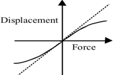
If the flesh/cushion system is regarded as substantially linear, then headband tension only affects leak performance and has no other influence. However, no spring is linear over an infinite range of excursions, as shown in Figure 16:
AUDIO AT HOME – AES 21ST UK CONFERENCE 2006
1 2
1
A AF res
C C
6
The gradient of the force/displacement curve determines spring compliance. A linear spring maintains constant compliance, whereas a non-linear spring will become more stiff as the headband tension is increased. Since both cushion and flesh compliance can be expected to behave in a non-linear manner, headband tension will have interesting effects on attenuation.
We have seen in Figure 14 that decreasing compliance will increase attenuation performance. With regard to headband tension, this suggests the unsurprising result that maximal tension is desired, since not only are leaks minimized but also cushion stiffness may be maximized, which will increase attenuation. Unfortunately, extreme values of headband tension rapidly become uncomfortable for users, and are likely to lead to rejection of a product regardless of its attenuation / reproduction performance.
In response to this dilemma, some manufacturers have adopted fluid-filled cushions (where a gel is used instead of a sponge element), since these have two
significant advantages. Firstly, the cushion moulds more effectively to the side of the head than a sponge type, meaning that leaks can be minimized without excessive headband tensions. Secondly, as long as sufficient tension is applied to overcome the compliance of whatever bag is used to contain the gel, and to hold the cup securely during normal head movements, then the lumped stiffness of the cushion is almost infinite. This means that flesh compliance rather than cushion compliance is the limiting factor in determining performance (Figure 17).
2.6 Limitations of the lumped-element technique
The lumped parameter technique has been shown to be effective in modelling the electro-acoustic performance of small drivers in headphones, and also of great utility in predicting the behaviour of headphone cups, cushions and leaks. However, circumstances sometimes arise where such models become less effective – most notably where the ‘lumped’ assumption breaks down within a given element, which starts to behave in a distributed manner.
Perhaps the most obvious example of this as applied to headphones is in the case of the ‘compliant’ volume of air under the cup. As is the case in room acoustics, this volume will behave as a lumped element as long as wavelength is long compared to enclosure dimensions – the so-called ‘zeroth mode’. Once wavelength decreases to approaching twice the largest dimension of the enclosure (assuming half-wave behaviour resulting from comparatively large boundary impedances) then the first resonant modes of the space will occur. Each mode is associated with
AUDIO AT HOME – AES 21ST UK CONFERENCE 2006
7 Figure 15: Degradation of protector performance due to small leak impedancesFigure 17: Attenuation performance of foam, and fluid (gel) cushions
Figure 16: Force / displacement characteristic for linear and non-linear springs
M.R AVIS AND L. J.KELLY
an eigenvalue – a resonant frequency – and a spatial eigenfunction – which dictates the variance of pressure and particle velocity throughout the enclosure. The fact of this variance tells us that our lumped assumption is no longer correct, and that as a result the performance of the system will differ from that expected.
Since circumaural headphones are small compared to listening rooms, we might expect a lumped assumption to perform well to a comparatively high frequency. However, a point is often reached where a more refined model is required. This may be because the modelled performance of a headphone differs significantly from ATF (Acoustic Test Fixture) or MIRE (Microphone In Real Ear) measurements, or it may be because (for instance with ANR (Active Noise Reducing) headsets) a very accurate map of the sound pressure under the cup is required in order to optimise the placement of error-sensing microphones.
In the case of the input impedance to the ear canal, an analytical distributed model was adopted from the outset (eq 1) since a lumped assumption in this case misses several important features. This distributed model was easily incorporated with the lumped models used for the remainder of the system. It is equally possible to attempt analytical models of the resonant behaviour of the volume of air under the headphone cup, and to incorporate these with the overall lumped scheme. Such models are introduced in section 3.
3.0 MODELING DISTRIBUTED PRESSURE UNDER HEAD SHELLS
3.1 Comparison between lumped and wave model
A simple example for the comparison of lumped-parameter and model modelling techniques is shown in Figure 18. Here, the cavity is reduced to a cylindrical pressure chamber, driven by a given velocity at one end.
The solution of the Helmholtz equation for this boundary value problem is well known and can be found, for example, in [6]. The solution is represented in equation (10).
n q m m q
q m
A
x
r
p
(
,
,
)
,
,
(10)We see a conventional summation of mode shapes (eigenfunctions) of the cylinder; modes in the longitudinal plane are represented by Ψn and modes in
the circular plane are represented by Ψm,q. Ψn form a
set of modes based on trigonometric functions which are harmonically related, and Ψm,q form a second set
which are based on the roots of a Bessel function, and which are not harmonically related. Am,q represents
the set of coefficients which determine the contribution of each mode to the overall response – effectively a set of modal ‘gain’ terms.
In the simple case of uniform excitation over the vibrating surface with rigid cavity walls, none of modes Ψm,q are excited and thus the response is
governed by a harmonic series of longitudinal trigonometric functions. For unit velocity excitation, the expression for the input impedance to the cavity is found as:
)
cot(
0
c
kL
j
Z
n
n
(11)This is the same result as that adopted for the input impedance to the ear canal, expressed in equation 2. It can be compared to a lumped model of the air in the
cavity as a simple compliance, the impedance of
AUDIO AT HOME – AES 21ST UK CONFERENCE 2006
8
foam
Ear canal wall
vibrating driver
cylinder
Figure 18: Coupling cavity simplified to cylindrical cavity
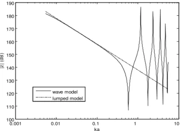
Figure 19: lumped vs. modal model for a cylindrical cavity
0.001 0.01 0.1 1 10
100 110 120 130 140 150 160 170 180 190
ka
|z
| (
dB
)
which is given in equation 3. Figure 19 compares these two formulations.
As we might expect, at high frequency the two models show significant divergence, and this can cause problems in the application cases previously mentioned.
3.2 Numerical methods
A modal decomposition approach may well yield satisfactory results for simple boundary geometries, but a headphone cavity is rarely in practice a perfect cylinder. In addition, its walls will exhibit complex and frequency-dependant boundary impedances, and the drive unit will excite the cavity over an area rather than as a point source. The problems may be soluble, but the complexity of the problem increases dramatically and the modal decomposition technique becomes less attractive.
Techniques exist that allow these problems to be solved more generally using numerical methods, the most common of these being the Finite Element Method (FEM) and the Boundary Element Method (BEM). Both FEM and BEM are based on a similar premise that the domain to be modelled is approximated by dividing it into small discrete sections or elements.
The principle behind FE methods are based on dividing the problem domain into N small elements. These elements coexist by means of continuity conditions, so that the behaviour of each element is determined by the behaviour of those elements immediately surrounding it. Elements which border a boundary or source are given relevant boundary conditions. In this manner we divide the problem into that of N small problems. The numerical scheme behind FEM requires the partial differential equation (PDE) governing each element to be rewritten into its ‘weak form’, and an approximation to the solution is developed and expressed as a sum of piecewise linear functions (or basis functions). In this form we have a system of N linear equations with N unknowns. This can be assembled into a matrix equation which can be solved, giving an approximate solution for each element or degree of freedom.
BEM is also concerned with dividing the problem into small elements, but it is slightly different in concept to FEM. BEM deals with the PDE by reducing it to a surface integral equation. The integral equation determines the value of the independent variable on the boundary surface due to contributions of sources within the domain and the scattering effect of the boundary itself. This provides enough information to
be able to solve the problem for any given point in the domain. Since BEM works in this manner, it requires only the boundary to be meshed rather than the full domain, thus reducing the degrees of freedom in the problem by an order of magnitude. BEM is not suitable for all types of problems however since it is limited to domains in which a Green’s function can be calculated, which restrict it to linear and homogenous media.
When using numerical methods for acoustics involving meshing a domain, it is important to ensure that the mesh is fine enough to accurately represent the wave patterns. Opinion varies but it is typically suggested that the mesh has a resolution of a minimum 8 elements per maximum wavelength. For a 3D mesh at full bandwidth, this can quickly lead to models with degrees of freedom in the order of millions. Due to computational expense, therefore, the application of numerical methods in acoustics has only recently been a practical option, and is still only really feasible in small sized or low frequency problems.
3.3 Application of numerical methods to headphone models
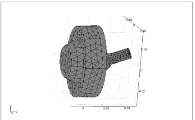
An ability to model wave behaviour in enclosed spaces with adaptable geometry opens up the possibility of full bandwidth 3D models of the sound fields under headphones. Figure 20 demonstrates a crude approximation of a coupling cavity mesh for a circumaural headphone. However as discussed in previous sections, headphones are more complex than the simple acoustic enclosure, and hence any model must be able to accommodate additional mechanical
coupling.
As an example, consider the cushion. An elementary numerical model may model the cushion as a locally
AUDIO AT HOME – AES 21ST UK CONFERENCE 2006
M.R AVIS AND L. J.KELLY
reacting surface and represent it as a known boundary impedance, with data obtained from measurement. This may be a reasonable approximation in some or even most circumstances. However, the admittance may not necessarily be locally reacting, there may be some significant coupling of the cavity with the cushion, or the cushion may be locally reacting but may present an impedance that varies with position.
A more complete model of the headphone would include a model of the cushion as a porous medium. Indeed this may be the only option if the headphone cushion extends to form a layer in front of the drive unit (as is the case with many supra-aural models). Several well-known approaches exist for modelling acoustic waves in porous media, which develop the problem with varying levels of rigour [7,8,9]. In general though, these models effectively represent the cushion as a lossy medium, characterised by its (complex) density and phase velocity. It should be noted that since BEM is limited to homogenous media a coupled cavity-cushion model using this method would not be possible.
Additionally, we might consider the headphone driver. So far the driver has been considered as executing pistonic motion. As has already been suggested, this is an approximation, especially at high frequencies. A thorough solution would include a structural model of the driver which could be coupled to the cavity, but this would be no trivial task.
A more convenient solution might ignore the coupling effects and present the driver as a complex vibrating surface which nonetheless retains constant velocity behaviour. Vibration data could be provided from measurement, necessitating laser interferometry, but this poses some difficulties since the diaphragms in question are small and frequently transparent. Additionally, the light mass of the diaphragm suggests that a constant velocity assumption could be considerably in error.
4.0 CONCLUSIONS
The design of a circum-aural headphone incorporating a dynamic driver has been described, using lumped parameter techniques. It has been shown that coupler volume affects the spectral response of the device, and that the choice of an open or closed back approach has significant influence on the affect of ‘leaks’, where the cushion makes an imperfect seal to the side of the head. The compliance of these cushions has been shown to be of primary importance in the attenuation of external sound fields through the cup, along with
the mass of the cup itself and the applied headband tension.
With the pressure field under a headphone cup becoming distributed at higher frequencies, a modal decomposition has been shown to give a more realistic representation than lumped parameters. For simple geometry a modal approach is possible analytically but for a headphone it is only feasible using numerical methods. Headphone issues such as structural coupling of the cushion and driver can be represented in a numerical model opening the possibility for headphone models which are accurate for the full audio bandwidth.
5.0 REFERENCES
[1] Beranek, L.L. ‘Acoustics’, American Inst. of Physics (New York 1986)
[2] Olson, H.F., ‘Elements of Acoustical Engineering’, Van Nostrand (New York 1947)
[3] Borwick, J., ‘Loudspeaker and Headphone Handbook’, 2nd Ed., Focal Press (Oxford 1994)
[4] Stimson, M.R., ‘The spatial distribution of sound pressure within scaled replicas of the human ear canal’, J.Acoust.Soc.Am. 78(5), 1985, pp1596-1602 [5] Kinsler, L.E., Frey, A.R. et al, ‘Fundamentals of Acoustics’, 4th Ed., Wiley (New York 2000)
[6] Morse, P.M. & Ingard, K.U. ‘Theoretical Acoustics’, (Princeton University Press, 1968) [7] Delany, M.E., Bazley, E.N. Acoustical properties of fibrous materials Applied Acoustics, 3 (1970) 105-16
[8] Biot, M.A. The theory of propagation of elastic waves in a fluid-saturated porous solid. I. Low frequency range. II. High frequency range. J.Acoust.Soc.Am 28 (1956) 168-91
[9] Allard, J.F. ‘Propagation of Sound in Porous Media’, Elsevier (London, 1993)
AUDIO AT HOME – AES 21ST UK CONFERENCE 2006