Solution of Volterra’s Integro-Differential Equations by Using Variational Iteration Method

(1)

Article

Solution of Volterra’s Integro-Differential Equations by

Using Variational Iteration Method

Abdulla – Al – Mamun 1,*, Weidong Tao 1, Md. Asaduzzaman 2

1_{School of Teacher Education, Huzhou Normal University, Zhejiang, China; [email protected]; [email protected]} 2_{Department of Mathematics, Islamic University, Kushtia, Bangladesh; [email protected]}

*_{Correspondence: [email protected]}

Abstract: In this paper, we introduce some basic idea of Variational iteration method for short (VIM) to solve the Volterra’s integro-differential equations. The VIM is used to solve effectively, easily, and accurately a large class of non-linear problems with approximations which converge rapidly to accurate solutions. For linear problems, it’s exact solution can be obtained by only one iteration step due to the fact that the Lagrange multiplier can be exactly identified. It is to be noted that the Lagrange multiplier reduces the iteration on integral operator and also minimizes the computational time. The method requires no transformation or linearization of any forms. Two numerical examples are presented to show the effectiveness and efficiency of the method. Also, we compare the result with the result from Homotopy perturbation method (HPM). Finally, we investigate the absolute difference between variational iteration method and homotopy perturbation method and draw the graph of difference function by using Mathematica.

Keywords: Variational iteration method, Integro-differential equation, Lagrange multiplier, Homotopy perturbation method.

1. Introduction

Volterra studied the hereditary influences when he was examining a population growth model. The research work resulted in a specific topic, where both differential and integral operators appeared together in the same equation. This new type of equations was termed as Volterra integro-differential equations, given in the form

𝑝( )(𝑥) = 𝑓(𝑥) + 𝜆 𝐾(𝑥, 𝑡)𝑝(𝑡) 𝑑𝑡, (1)

Where 𝑝( )_{(𝑥) =} _{. Because the resulted equation in (1) combines the differential operator and the integral}

operator, then it is necessary to define initial conditions 𝑝(0), 𝑝′(0), . . . , 𝑝 (0) for the determination of the

particular solution p(x) of the Volterra integro-differential equation (1). Any Volterra integro-differential equation is characterized by the existence of one or more of the derivatives 𝑝 (𝑥), 𝑝 (𝑥), . … … …. outside the integral sign. The

Volterra integro-differential equations may be observed when we convert an initial value problem to an integral equation by using Leibnitz rule. The Volterra integro-differential equation appeared after its establishment by Volterra. It then appeared in many physical applications such as glass forming process [1], nano-hydrodynamics [2], heat transfer, diffusion process in general, neutron diffusion and biological species coexisting together with increasing and decreasing rates of generating, and wind ripple in the desert. More details about the sources where these equations arise can be found in physics, biology and engineering applications books. To determine a solution for the integro-differential equation, the initial conditions should be given, and this may be clearly seen as a result of involving p(x) and its derivatives. The initial conditions are needed to determine the exact solution.

(2)

There are various numerical and analytical methods to solve such problems, for example, the homotopy perturbation method [3], the Adomian decomposition method [4], but each method limits to a special class of integro-differential equations. J.H. He used the variational iteration method for solving some integro-differential equations [5]. This Chinese mathematician chooses [5] initial approximate solution in the form of exact solution with unknown constants. M. Ghasemi et al solved the nonlinear Volterra's integro-differential equations [6] by using homotopy perturbation method. In [7], the variational iteration method was applied to solve the system of linear integro-differential equations. Also, J. Biazar et al solved systems of integro-differential equations by He's homotopy perturbation method [8].

2. History of Variation Method (VIM)

The variational iteration method (VIM) developed in 1999 by He in [9-18] will be used to study the linear wave equation, nonlinear wave equation, and wave-like equation in bounded and unbounded domains. The method has been proved by many authors [19-31] to be reliable and efficient for a wide variety of scientific applications, linear and nonlinear as well. It was shown by many authors that this method is more powerful than existing techniques such as the Adomian method [32,33], perturbation method, etc. The method gives rapidly convergent successive approximations of the exact solution if such a solution exists; otherwise a few approximations can be used for numerical purposes. The method is effectively used in [10-25] and the references therein. The perturbation method suffers from the computational workload, especially when the degree of nonlinearity increases. Moreover, the Adomian method suffers from the complicated algorithms used to calculate the Adomian polynomials that are necessary for nonlinear problems. The VIM has no specific requirements, such as linearization, small parameters, etc. for nonlinear operators.

The variational iteration method, which is a modified general Lagrange multiplier method [34] has been shown to solve effectively, easily and accurately, a large class of nonlinear problems with approximations which converge quickly to accurate solutions. It was successfully applied to autonomous ordinary differential equation [13], to nonlinear partial differential equations with variable coefficients [35], to Schrödinger-KDV, generalized KDV and shallow water equations [36], to Burgers' and coupled Burgers' equations [37], to the linear Helmoltz partial differential equation [38] and recently to nonlinear fractional differential equations with Caputo differential derivative [39], and other fields [10,20,40,41-44]. On the other hand, one of the interesting topics among researchers is solving integro-differential equations.

3. Variational Iteration Method for Solving Volterra’s Integro-Differential Equations

The purpose of this paper is to extend the analysis of the variational iteration method to solve the system of general nonlinear Volterra’s integro-differential equations which is as follows:

𝑝( )(𝑥) = 𝐻 𝑥, 𝑝 (𝑥), … . , 𝑝( )(𝑥), 𝑝 (𝑥), … . , 𝑝( )(𝑥), … … … . , 𝑝 (𝑥), … . , 𝑝( )(𝑥)

+ 𝐾 𝑥, 𝑡, 𝑝 (𝑡), … . , 𝑝( )(𝑡), … … … , 𝑝 (𝑡), … . , 𝑝( )(𝑡) 𝑑𝑡

⋮ ⋮ ⋮ ⋮ ⋮ ⋮ ⋮ ⋮ ⋮ ⋮ ⋮⋮ ⋮ ⋮ ⋮ ⋮ ⋮ ⋮ ⋮ ⋮ ⋮ ⋮

+ 𝐾 𝑥, 𝑡, 𝑝 (𝑡), … . , 𝑝( )(𝑡), … … … , 𝑝 (𝑡), … . , 𝑝( )(𝑡) 𝑑𝑡

⎭ ⎪ ⎪ ⎪ ⎪ ⎪ ⎪ ⎬ ⎪ ⎪ ⎪ ⎪ ⎪ ⎪ ⎫

(2)

(3)

For solving the above system by the variational iterative method, for simplicity, we consider all of terms as restricted variation except 𝑝( )(𝑥), 𝑖 = 1,2,3, … … … … , 𝑛. According to the variational iterative method, we derive

correction functional as follows:

𝑝, (𝑥)

= 𝑝, (𝑥) + 𝜆 (𝑠) [𝑝, ( )

(𝑠)

− 𝐻 (𝑠, 𝑝, (𝑠), … … , 𝑝, ( )

(𝑠)), … … , 𝑝 , (𝑠), … … , 𝑝 , ( )

(𝑠)), 𝑝 , (𝑠), … … , 𝑝 , ( )

(𝑠)), … … , 𝑝 , (𝑠), … … , 𝑝 , ( )

(𝑠))

− 𝐾 (𝑠, 𝑡, 𝑝, (𝑡), … … , 𝑝, ( )

(𝑡), … … , 𝑝 , (𝑡), … … , 𝑝 , ( )

(𝑡))𝑑𝑡]𝑑𝑠

For 𝑖 = 1,2,3, … … , 𝑛 and the stationary conditions of the above correction functional can be expressed as follows: 𝜆( )(𝑠) = 0

1 − (−1) 𝜆( )(𝑠) = 0

𝜆( )(𝑠) = 0, 𝑗 = 1,2,3, … … , 𝑚 − 2, 𝑖 = 1,2,3, … … , 𝑛 𝜆 (𝑠)| = 0

The Lagrange multiplier, therefore, can be identified as follows:

𝜆 (𝑠) = (−1)

(𝑚 − 1)!(𝑠 − 𝑥)

As a result, we obtain the following iteration formulas

𝑝, (𝑥)

= 𝑝, (𝑥) +

(−1)

(𝑚 − 1)!(𝑠 − 𝑥) [𝑝, ( )_(𝑠)

− 𝐻 (𝑠, 𝑝, (𝑠), … … , 𝑝, ( )

(𝑠)), … … , 𝑝 , (𝑠), … … , 𝑝 , ( )

(𝑠)), 𝑝 , (𝑠), … … , 𝑝 , ( )

(𝑠)), … … , 𝑝 , (𝑠), … … , 𝑝 , ( )

(𝑠))

− 𝐾 (𝑠, 𝑡, 𝑝, (𝑡), … … , 𝑝, ( )

(𝑡), … … , 𝑝 , (𝑡), … … , 𝑝 , ( )

(𝑡))𝑑𝑡]𝑑𝑠

4. Numerical Examples for Seventh Order Boundary Value Problem by Using VIM

In this section, we present two examples to show efficiency and high accuracy of the variational iteration method for solving Volterra integro-differential equations.

Example 01 Let us consider the system of integro-differential equations as follows:

⎩ ⎪ ⎨ ⎪

⎧ _{𝑝 (𝑥) = −1 − 𝑥 − sin 𝑥 +} _{𝑝(𝑡) + 𝑞(𝑡) 𝑑𝑡}

𝑞 (𝑥) = 1 − 2 − sin 𝑥 − cos 𝑥 + 𝑝(𝑡) − 𝑞(𝑡) 𝑑𝑡

Subjected to the initial conditions: 𝑝(0) = 1, 𝑝 (0) = 1, 𝑞(0) = 0, 𝑞 (0) = 2

With the exact solutions

𝑝(𝑥) = 𝑥 + cos 𝑥 , 𝑞(𝑥) = 𝑥 + sin 𝑥

According to VIM we have following iteration formulas

𝑝 (𝑥) = 𝑝 (𝑥) + (𝑠 − 𝑥) 𝑝 (𝑠) + 1 + 𝑠 + sin 𝑠 − 𝑝 (𝑡) + 𝑞 (𝑡) 𝑑𝑡 𝑑𝑠

(4)

Now, we choose initial approximations 𝑝 (𝑥) = 1 + 𝑥 and 𝑞 (𝑥) = 2𝑥 which satisfy initial conditions then, we get

𝑝 (𝑥) = 1 + 𝑥 + (𝑥 − 𝑡)(−1 − 𝑡 − sin 𝑡 + (1 + 3𝑇)𝑑𝑇)𝑑𝑡 = 1 + 𝑥 + (𝑥 − 𝑡) −1 − 𝑡 − sin 𝑡 + 𝑡 +3 2𝑡 𝑑𝑡

= 1 + 𝑥 + (𝑥 − 𝑡) −1 + 𝑡 +1

2𝑡 − sin 𝑡 𝑑𝑡

= 1 + 𝑥 + 𝑥 −𝑥 +1 2𝑥 +

1

6𝑥 + cos 𝑥 − 1 − − 1 2𝑥 +

1 3𝑥 +

1

8𝑥 + 𝑥 cos 𝑥 − sin 𝑥 = 1 −1

2𝑥 + 1 6𝑥 +

1

24𝑥 + sin 𝑥 ∴ 𝑝 (𝑥) = 1 −1

2!𝑥 + 1 3!𝑥 +

1

4!𝑥 + sin 𝑥

𝑞 (𝑥) = 2𝑥 + (𝑥 − 𝑡) 1 − 2 − sin 𝑡 − cos 𝑡 + (1 − 𝑇)𝑑𝑇 𝑑𝑡 = 2𝑥 + (𝑥 − 𝑡) −1 + 𝑡 −1

2𝑡 − sin 𝑡 − cos 𝑡 𝑑𝑡

= 2𝑥 + 𝑥 −𝑥 +1 2𝑥 −

1

6𝑥 + cos 𝑥 − 1 − sin 𝑥 − −1

2𝑥 + 1 3𝑥 −

1

8𝑥 + 𝑥 cos 𝑥 − sin 𝑥 − 𝑥 sin 𝑥 − cos 𝑥 + 1 = 2𝑥 −1

2𝑥 + 1 6𝑥 −

1

24𝑥 − 𝑥 + sin 𝑥 + cos 𝑥 − 1 = −1 + 𝑥 − 1 2𝑥 +

1 6𝑥 −

1

24𝑥 + sin 𝑥 + cos 𝑥 ∴ 𝑞 (𝑥) = −1 + 𝑥 −1

2!𝑥 + 1 3!𝑥 −

1

4!𝑥 + sin 𝑥 + cos 𝑥

Similarly,

𝑝 (𝑥) = 𝑥 + 1 −1 2!𝑥 +

1 4!𝑥 −

1

6!𝑥 + ⋯ … … … 𝑞 (𝑥) = 𝑥 + 𝑥 −1

3!𝑥 + 1 5!𝑥 −

1

7!𝑥 + ⋯ … … …

Thus, the closed from solution are as follows:

𝑝(𝑥) = lim

→ 𝑝 (𝑥) = 𝑥 + cos 𝑥 𝑞(𝑥) = lim

→ 𝑞 (𝑥) = 𝑥 + sin 𝑥

This example has been solved by homotopy perturbation method in [45]. The solutions of this example by homotopy perturbation method (HPM) are obtained as:

𝑝(𝑥) = 4 + 𝑥 − 2𝑥 +𝑥 6 −

𝑥 180+

𝑥 10080−

𝑥 907200−

𝑥

1556755200− 3 cos 𝑥

𝑞(𝑥) = 5𝑥 −2𝑥 3 +

𝑥 30−

𝑥 1260+

𝑥 90720−

𝑥 9979200−

𝑥

1556755200− 3 sin 𝑥

Example 02 Consider the following system of nonlinear integro-differential equations:

𝑝 (𝑥) = 1 −1 3𝑥 −

1

2𝑞 (𝑥) + 1

2 (𝑝 (𝑡) + 𝑞 (𝑡))𝑑𝑡

𝑞 (𝑥) = −1 + 𝑥 − 𝑥𝑝(𝑥) +1

4 (𝑝 (𝑡) − 𝑞 (𝑡))𝑑𝑡 _⎭⎪ ⎬ ⎪ ⎫

Subject to the initial conditions:

𝑝(0) = 1, 𝑝 (0) = 2, 𝑞(0) = −1, 𝑞 (0) = 0

(5)

𝑝 (𝑥) = 𝑝 (𝑥) + (𝑥 − 𝑡)(1 −1 3𝑡 −

1

2𝑞 (𝑡) + 1

2 (𝑝 (𝑇) + 𝑞 (𝑇))𝑑𝑇)𝑑𝑡

𝑞 (𝑥) = 𝑞 (𝑥) + (𝑥 − 𝑡)(−1 + 𝑡 − 𝑡𝑝(𝑡) +1

4 (𝑝 (𝑇) − 𝑞 (𝑇))𝑑𝑇)𝑑𝑡 _⎭⎪ ⎬ ⎪ ⎫

Where 𝑝 (𝑥) = 2𝑥 + 1, 𝑞 (𝑥) = 1 and 𝑝 (𝑥), 𝑞 (𝑥) indicates the nth approximation of 𝑝(𝑥) and 𝑞(𝑥) respectively.

Now,

𝑝 (𝑥) = 2𝑥 + 1 + (𝑥 − 𝑡)(1 −1 3𝑡 +

1

2 (4𝑇 + 4𝑇 + 2)𝑑𝑇)𝑑𝑡

= 2𝑥 + 1 + (𝑥 − 𝑡) 1 −1 3𝑡 +

1 2

4

3𝑡 + 2𝑡 + 2𝑡 𝑑𝑡

= 2𝑥 + 1 + (𝑥 − 𝑡) 1 −1 3𝑡 +

2

3𝑡 + 𝑡 + 𝑡 𝑑𝑡 = 2𝑥 + 1 + (𝑥 − 𝑡) 1 + 1

3𝑡 + 𝑡 + 𝑡 𝑑𝑡

= 2𝑥 + 1 + 𝑥 + 1 12𝑥 +

1 3𝑥 +

1 2𝑥 −

1 2𝑥 +

1 15𝑥 +

1 4𝑥 +

1 3𝑥 = 1 + 2𝑥 +1

2𝑥 + 1 6𝑥 +

1 12𝑥 +

1 60𝑥 ∴ 𝑝 (𝑥) = 1 + 2𝑥 +1

2𝑥 + 1 6𝑥 +

1 12𝑥 +

1 60𝑥

𝑞 (𝑥) = 1 + (𝑥 − 𝑡)(−1 + 𝑡 − 𝑡(2𝑡 + 1) +1

4 (4𝑇 + 4𝑇)𝑑𝑇)𝑑𝑡

= 1 + (𝑥 − 𝑡) −1 + 𝑡 − 2𝑡 − 𝑡 +1 4

4

3𝑡 + 2𝑡 𝑑𝑡

= 1 + (𝑥 − 𝑡) −1 − 𝑡 − 𝑡 +1 3𝑡 +

1

2𝑡 𝑑𝑡 = 1 + (𝑥 − 𝑡) −1 − 1

2𝑡 − 𝑡 + 1 3𝑡 𝑑𝑡

= 1 + −𝑥 −1 6𝑥 −

1 2𝑥 +

1

12𝑥 − − 1 2𝑥 −

1 8𝑥 −

1 3𝑥 +

1 15𝑥 = 1 −1

2𝑥 − 1 6𝑥 −

1 24𝑥 +

1 60𝑥 ∴ 𝑞 (𝑥) = 1 −1

2𝑥 − 1 6𝑥 −

1 24𝑥 +

1 60𝑥

Similarly,

𝑝 (𝑥) = 1 + 2𝑥 +1 2𝑥 +

1 6𝑥 +

1 24𝑥 +

1 120𝑥 +

1 720𝑥 +

17 5040𝑥 +

1 672𝑥 +

53 120960𝑥 −

1 103680𝑥

+ 1

228096𝑥 + 1

1900800𝑥 + 1 6177600𝑥 𝑞 (𝑥) = −1 −1

2𝑥 − 1 6𝑥 −

1 24𝑥 −

1 120𝑥 −

1 720𝑥 −

11 10080𝑥 +

13 241920𝑥 +

17

1036800𝑥 + 47 11404800𝑥

+ 1

1267200𝑥

and so on.

Thus, the closed from solution are as follows:

𝑝(𝑥) = lim

→ 𝑝 (𝑥) = 𝑥 + 𝑒 𝑞(𝑥) = lim

→ 𝑞 (𝑥) = 𝑥 − 𝑒

(6)

𝑝(𝑥) = 1 + 2𝑥 +

2𝑥 +6𝑥 +24𝑥 +120𝑥 + ⋯ … … …. 𝑞(𝑥) = −1 −1

2𝑥 − 1 6𝑥 −

1 24𝑥 −

1

120𝑥 − ⋯ … … … ..

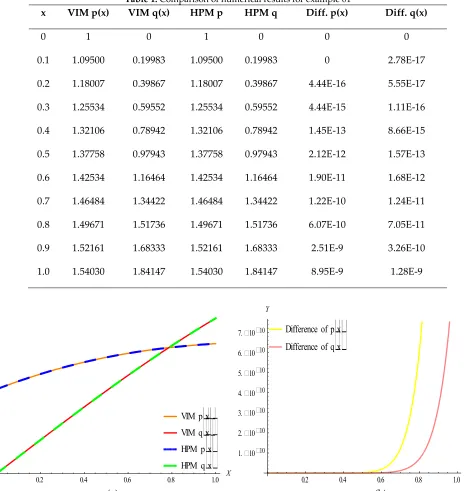
Table 1. Comparison of numerical results for example 01

x VIM p(x) VIM q(x) HPM p HPM q Diff. p(x) Diff. q(x)

0 0.1 0.2 0.3 0.4 0.5 0.6 0.7 0.8 0.9 1.0

1 1.09500 1.18007 1.25534 1.32106 1.37758 1.42534 1.46484 1.49671 1.52161 1.54030

0 0.19983 0.39867 0.59552 0.78942 0.97943 1.16464 1.34422 1.51736 1.68333 1.84147

1 1.09500 1.18007 1.25534 1.32106 1.37758 1.42534 1.46484 1.49671 1.52161 1.54030

0 0.19983 0.39867 0.59552 0.78942 0.97943 1.16464 1.34422 1.51736 1.68333 1.84147

0 0 4.44E-16 4.44E-15 1.45E-13 2.12E-12 1.90E-11 1.22E-10 6.07E-10 2.51E-9 8.95E-9

0 2.78E-17 5.55E-17 1.11E-16 8.66E-15 1.57E-13 1.68E-12 1.24E-11 7.05E-11 3.26E-10 1.28E-9

(a) (b)

Figure 1. Comparison of numerical results for example 01: (a) Comparison of VIM with HPM; (b) Absolute difference between VIM & HPM.

VIM p



x



VIM q



x



HPM p



x



HPM q



x



0.2 0.4 0.6 0.8 1.0 X

0.5 1.0 1.5

Y

Difference of p



x



Difference of q



x



0.2 0.4 0.6 0.8 1.0 X 1.1010

2.1010 3.1010 4.1010 5.1010 6.1010 7.1010

(7)

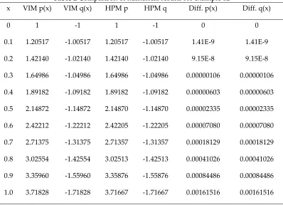
Table 2 Comparison of numerical results for example 02

x VIM p(x) VIM q(x) HPM p HPM q Diff. p(x) Diff. q(x) 0

0.1 0.2 0.3 0.4 0.5 0.6 0.7 0.8 0.9 1.0

1 1.20517 1.42140 1.64986 1.89182 2.14872 2.42212 2.71375 3.02554 3.35960 3.71828

-1 -1.00517 -1.02140 -1.04986 -1.09182 -1.14872 -1.22212 -1.31375 -1.42554 -1.55960 -1.71828

1 1.20517 1.42140 1.64986 1.89182 2.14870 2.42205 2.71357 3.02513 3.35876 3.71667

-1 -1.00517 -1.02140 -1.04986 -1.09182 -1.14870 -1.22205 -1.31357 -1.42513 -1.55876 -1.71667

0 1.41E-9 9.15E-8 0.00000106 0.00000603 0.00002335 0.00007080 0.00018129 0.00041026 0.00084486 0.00161516

(a) (b)

Figure 2. Comparison of numerical results for example 02: (a) Comparison of VIM with HPM; (b) Absolute difference between VIM & HPM.

5. Conclusion

In this paper, we applied the Variational Iteration Method (VIM) for solving the systems of Volterra integro-differential equations. It is important to point out that some other methods should be applied for systems with separable or difference kernels. Whereas, the VIM can be used for solving systems of Volterra integro-differential equations with any kind of kernels. By comparing the results of other numerical methods such as homotopy perturbation method, we conclude that the VIM is more accurate, fast and reliable. Besides, VIM does not require

VIM p



x



VIM q



x



HPM p



x



HPM q



x



0.2 0.4 0.6 0.8 1.0 X

1 1 2 3

Y

Difference of p



x



Difference of q



x



0.2 0.4 0.6 0.8 1.0 X

0.0002 0.0004 0.0006 0.0008 0.0010

(8)

small parameters; thus, the limitations of the traditional perturbation methods can be eliminated, and the calculations are also simple and straight forward. These advantages has been confirmed by employing two examples. Therefore, this method is a very effective tool for calculating the exact solutions of systems of integro-differential equations.

Author Contributions: These authors contributed equally to this work.

Conflicts of Interest: The authors declare no conflict of interest.

References

1. H. Wang, H. M. Fu, H. F. Zhang, et al., A practical thermodynamic method to calculate the best glass-forming composition for bulk metallic glasses, Int. J. Nonlinear Sci. Numer. Simul. 8 (2) (2007) 171-178.

2. L. Xu, J. H. He, Y. Liu, Electrospun nanoporous spheres with Chinese drug, Int. J. Nonlinear Sci. Numer. Simul. 8 (2) (2007) 199-202.

3. M. El-Shahed, Application of He’s homotopy perturbation method to Volterra’s integro differential equation, Int. J. Nonlinear Sci. Numer. Simul. 6 (2) (2005) 163-168.

4. S. M. El-Sayed, D. Kaya, S. Zarea, The decomposition method applied to solve higher order linear Volterra-Fredholm integro-differential equations, Int. J. Nonlinear Sci. Numer. Simul. 5 (2) (2004) 105-112.

5. S. Q. Wang, J. H. He, Variational iteration method for solving integro-differential equation, Phys. Lett. A 367 (2007) 188-191. 6. J. Biazar, Solution of systems of integro-differential equations by Adomian decomposition method, Appl. Math. Comput.

168 (2005) 1232-1238.

7. J. Saberi-Nadjafi, M. Tamamgar, The variational iteration method: A highly promising method for solving the system of integro-differential equations, Comput. Math. Appl., (Article in press).

8. J. Biazar, H. Hhazvini, M. Eslami, He’s homotopy perturbation method for system of integro-differential equations, Chaos, Solitons \& Fractals (Article in press).

9. J.H. He, Some asymptotic methods for strongly nonlinear equations, Int. J. Modern Phys. B 20 (10) (2006) 1141–1199. 10. J.H. He, Non-perturbative methods for strongly nonlinear problems, Dissertation.de-Verlag im Internet GmbH, Berlin,

2006.

11. J.H. He, Approximate analytical solution for seepage flow with fractional derivatives in porous media, Comput. Methods Appl. Mech. Engrg.167 (1998) 57–68.

12. J.H. He, Variational iteration method for autonomous ordinary differential systems, Appl. Math. Comput. 114 (2/3) (2000) 115–123.

13. J.H. He, X.H. Wu, Construction of solitary solution and compacton-like solution by variational iteration method, Chaos Solitons Fractals 29 (1) (2006) 108–113.

14. J.H. He, A new approach to nonlinear partial differential equations, Commun. Nonlinear Sci. Numer. Simul. 2 (4) (1997) 203–205.

15. J.H. He, A variational iteration approach to nonlinear problems and its applications, Mech. Appl. 20 (1) (1998) 30–31 (in Chinese).

16. J.H. He, Variational iteration method—a kind of nonlinear analytical technique: Some examples, Int. J. Nonlinear Mech. 34 (1999) 699–708.

17. J.H. He, A generalized variational principle in micromorphic thermoelasticity, Mech. Res. Commun. 32 (2005) 93–98. 18. J.H. He, Variational iteration method—some recent results and new interpretations, J. Comput. Appl. Math. (2006) (in

press).

19. A.A. Mamun, M. Asaduzzaman, Solution of seventh order boundary value problem by using variational iteration method, Int. J. of Mathematics and computational science, Vol. 5, No. 1, 2019, pp. 6-12, ISSN: 2381-7011 (Print); ISSN: 2381-702X (Online), Published online: April 17, 2019.

20. E.M. Abulwafa, M.A. Abdou, A.A. Mahmoud, The solution of nonlinear coagulation problem with mass loss, Chaos Solitons Fractals 29 (2006) 313–330.

21. S. Momani, Z. Odibat, Analytical approach to linear fractional partial differential equations arising in fluid mechanics, Phys. Lett. A 1 (53) (2006)1–9.

22. S. Momani, S. Abusaad, Application of He’s variational-iteration method to Helmholtz equation, Chaos Solitons Fractals 27 (5) (2005) 1119–1123.

(9)

24. A.M. Wazwaz, A comparison between the variational iteration method and Adomian decomposition method, J. Comput. Appl. Math. (2006) (in press).

25. A.M. Wazwaz, The variational iteration method for rational solutions for KdV, K(2,2), Burgers, and cubic Boussinesq equations, J. Comput. Appl. Math. (2006) (in press).

26. A.M. Wazwaz, Partial Differential Equations: Methods and Applications, Balkema Publishers, The Netherlands, 2002. 27. A.M. Wazwaz, Necessary conditions for the appearance of noise terms in decomposition solution series, Appl. Math.

Comput. 81 (1997) 265–274.

28. A.M.Wazwaz, A new technique for calculating Adomian polynomials for nonlinear polynomials, Appl. Math. Comput. 111 (1) (2000) 33–51.

29. A.M. Wazwaz, A new method for solving singular initial value problems in the second order differential equations, Appl. Math. Comput. 128 (2002) 47–57.

30. A.M Wazwaz, A First Course in Integral Equations, World Scientific, Singapore, 1997.

31. A.M. Wazwaz, Analytical approximations and Pad´e approximants for Volterra’s population model, Appl. Math. Comput. 100 (1999) 13–25.

32. G. Adomian, Solving Frontier Problems of Physics: The Decomposition Method, Kluwer, Boston, 1994.

33. G. Adomian, A review of the decomposition method in applied mathematics, J. Math. Anal. Appl. 135 (1988) 501–544. 34. M. Inokuti et al. General use of the Lagrange multiplier in nonlinear mathematical physics, in: S. Nemat-Nassed, ed.,

Variational method in the Mechanics of Solids (Pergamon Press, 1978) 156-162.

35. J. H. He, Variational principle for some nonlinear partial differential equations with variable coefficients, Chaos, Solitons \& Fractals 19 (2004) 847-851.

36. M. A. Abdou, A.A. Soliman, New applications of variational iteration method, Physica D 211 (1-2) (2005) 1-8.

37. M. A. Abdou, A.A. Soliman, Variational iteration method for solving Burger’s and coupled Burger’s equations, J. comput. Appl. Math. 181 (2005) 245-251.

38. S. Momani, S. Abuasad, Application of He’s variational iteration method to Helmholtz equation, Chaos, Solitons \& Fractals 27 (2006) 1119-1123.

39. Z. M. Odibat, S. Momani, Application of variational iteration method to nonlinear differential equations of fractional order, Int. J. Nonlinear Sci. Numer. Simul. 7 (2006) 27-36.

40. N. Bildik, A. Konuralp, The use of variational iteration method, differential transform method and Adomian decomposition method for solving different types of nonlinear partial differential equations, Int. J. Nonlinear Sci. Numer. Simul. 7(1) (2006) 65-70.

41. M. Dehghan, M. Tatari, Identifying an unknown function in a parabolic equation with overspecified data via He’s variational iteration method, Chaos, Solitons and Fractals, Volume 36, (2008), 157-166.

42. M. Dehgha, F. Shakeri, Application of He’s variational iteration method for solving the Cauchy reaction-diffusion problem, Journal of Computational and Applied Mathematics, Volume 214, (2008), 435-446.

43. M. Dehgha, F. Shakeri, Numerical solution of a biological population model using He’s variational iteration method, Computers and Mathematics with Applications, 54 (2007) 1197-1209.

44. M. Dehgha, F. Shakeri, Approximate solution of a differential equation arising in astrophysics using the variational iteration method, New Astronomy, 13 (2008) 53-59.