How to Make a Mudsparkler

(1)

University of South Carolina

Scholar Commons

Theses and Dissertations

2017

Multi-Model Structural Analysis

Wesley Holt

University of South Carolina

Follow this and additional works at:https://scholarcommons.sc.edu/etd

Part of theCivil Engineering Commons

This Open Access Thesis is brought to you by Scholar Commons. It has been accepted for inclusion in Theses and Dissertations by an authorized administrator of Scholar Commons. For more information, please [email protected].

Recommended Citation

(2)

Multi-Model Structural Analysis

by

Wesley Holt

Bachelor of Science

Tennessee Technological University 2007

Submitted in Partial Fulfillment of the Requirements

for the Degree of Master of Science in

Civil Engineering

College of Engineering and Computing

University of South Carolina

2017

Accepted by:

Juan Caicedo, Director of Thesis

Dimitris Rizos, Reader

Paul Ziehl, Reader

(3)

c

Copyright by Wesley Holt, 2017

(4)

Acknowledgments

I would like to sincerely thank my advisor, Dr Juan Caicedo, for his guidance,

ex-pertise, and extremely valuable time. I would also like to thank my thesis committee

(5)

Abstract

The uncertainty in modeling earthquake loading is investigated through the

compar-ison of various openSEES models. A series of models is created and the responses

compared with each other as well as with a full scale shake table experiment. The

openSEES models selected for comparison include two linear models, a nonlinear

model using the Steel01 material for the entire cross section, and eight fiber models

using reinforcing steel material and various concrete materials.

The models are subjected to a series of nine simulated earthquakes, matching

the excitations applied to the shake table test. It is found that all of the models

under-predict the maximum base reactions. However, the nonlinear model using the

Steel01 material generates the most accurate response of the models tested. It is seen

that accumulated damage from each excitation affects the response of the column

during the subsequent excitations and that the effect of this accumulated damage

contributes to the total amount of uncertainty in the models.

A method of combining the responses of the different models to create a single

probabilistic output is presented and some potential real world challenges to

(6)

List of Tables

Table 2.1 Model Types . . . 8

Table 2.2 Parameters used for Model 1 . . . 9

Table 2.5 Moment-Curvature Data . . . 12

Table 2.7 Model 4 and Model 5 materials . . . 14

Table 2.8 Parameters used for fiber materials in model 4 and model 5 . . . . 15

Table 2.10 Parameters used for Bond-SP01 material . . . 19

Table 3.1 Maximum Base Moment . . . 41

Table 3.2 Maximum Base Shear . . . 42

Table 3.3 Maximum Deflection . . . 45

Table 3.4 Relative weights assigned to the openSEES models . . . 49

Table 3.5 Parameters used to estimate the column response using hand methods 53 Table 3.6 Sa and Sd values for Tn = 1.15 from Figures 3.37, 3.38, and 3.39 . 54 Table 3.7 Resulting Base Reactions from EQ 1, 2, & 3 based on linear single degree of freedom model [14], [15] . . . 55

(11)

List of Figures

Figure 1.1 PEER contest predictions of maximum displacement at the top

of column verses measured response [1] . . . 4

Figure 1.2 PEER contest predictions of maximum moment at the base of the column verses measured response [1] . . . 4

Figure 2.1 Pier Cross Section Details [2] . . . 7

Figure 2.2 Comparison of maximum displacement and the number of elas-tic elements . . . 10

Figure 2.3 Moment-Curvature of Column at Different Loading Stages . . . . 12

Figure 2.4 Concrete01 (Source: OpenSees documentation) . . . 16

Figure 3.1 Maximum base shear of all models . . . 23

Figure 3.2 Maximum base moment of all models . . . 24

Figure 3.3 Maximum deflection of all models . . . 25

Figure 3.4 Comparing the time domain simulations of models 1 (blue) and 2 (green) for EQ 1 . . . 25

Figure 3.5 Comparing the time domain simulations of models 1 (blue) and 2(green) for EQ 5 . . . 26

(12)

Figure 3.7 Maximum base shear of model 3 compared with the

experimen-tal results . . . 28

Figure 3.8 Maximum base moment omitting models 1 and 2 . . . 29

Figure 3.9 Maximum base moment of model 3 compared with the experi-mental results . . . 30

Figure 3.10 Maximum deflection omitting models 1 and 2 . . . 32

Figure 3.11 Maximum deflection of model 3 compared with the experimen-tal results . . . 33

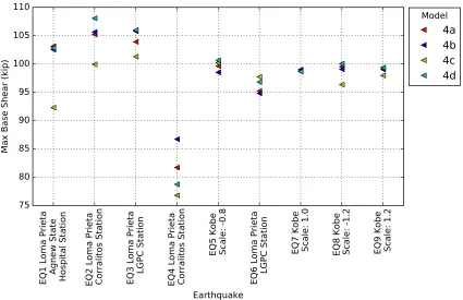
Figure 3.12 Comparing maximum base shear of models 4a, 4b, 4c, and 4d . . 34

Figure 3.13 Comparing maximum base moment of models 4a, 4b, 4c, and 4d . 35 Figure 3.14 Comparing maximum deflection of models 4a, 4b, 4c, and 4d . . . 36

Figure 3.16 Comparing maximum base moment of models 5a, 5b, 5c, and 5d . 37 Figure 3.17 Comparing maximum deflection of models 5a, 5b, 5c, and 5d . . . 37

Figure 3.18 Moment-curvature plot of EQ2 generated from the PEER ex-periment [2] . . . 38

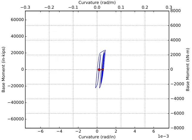
Figure 3.22 Moment-curvature plot of EQ2 generated from model 3 . . . 42

(13)

Figure 3.26 Moment-Curvature Plot of EQ4 generated from model 4a . . . 44

Figure 3.27 Moment-Curvature Plot of EQ5 generated from model 4a . . . 45

Figure 3.29 Prior prediction combination of maximum base shear generated from models 4a, 4b, 4c, and 4d. Red markers indicate

experi-mental results. . . 48

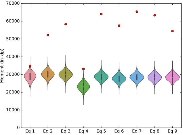
Figure 3.30 Prior prediction combination of maximum base moment gen-erated from models 4a, 4b, 4c, and 4d. Red markers indicate

experimental results. . . 49

Figure 3.31 Prior prediction combination of maximum base shear generated from models 5a, 5b, 5c, and 5d. Red markers indicate

experi-mental results. . . 50

Figure 3.32 Prior prediction combination of maximum base moment gen-erated from models 5a, 5b, 5c, and 5d. Red markers indicate

experimental results. . . 50

Figure 3.33 Prior prediction combination of maximum base shear generated from models 4a, 4b, 4c, 4d, 5a, 5b, 5c, and 5d. Red markers

indicate experimental results. . . 51

Figure 3.34 Prior prediction combination of maximum base moment gen-erated from models 4a, 4b, 4c, 4d, 5a, 5b, 5c, and 5d. Red

markers indicate experimental results. . . 51

Figure 3.35 Prior prediction combination of maximum base shear generated from models 3, 4a, 4b, 4c, 4d, 5a, 5b, 5c, and 5d. Red markers

indicate experimental results. . . 52

Figure 3.36 Prior prediction combination of maximum base moment gener-ated from models 3, 4a, 4b, 4c, 4d, 5a, 5b, 5c, and 5d. Red

markers indicate experimental results. . . 52

Figure 3.37 EQ1 pseudo-acceleration and displacement response spectra at

1% damping ratio [3] . . . 53

(14)

1% damping ratio [3] . . . 54

Figure 4.1 Maximum Base Shear omitting models 1 and 2 . . . 59

Figure 4.2 Maximum Base Moment omitting models 1 and 2 . . . 59

Figure 4.3 Maximum Column Deflection omitting models 1 and 2 . . . 60

Figure A.1 Input excitation for EQ1 [1] . . . 67

Figure B.1 Displacement response of model 1 for EQ1 . . . 72

(15)

Figure B.10 Fx response of model 1 for EQ1 . . . 77

Figure B.19 Mz response of model 1 for EQ1 . . . 81

Figure C.1 Displacement response of model 2 for EQ1 . . . 86

(16)

Figure C.10 Fx response of model 2 for EQ1 . . . 91

Figure C.19 Mz response of model 2 for EQ1 . . . 95

(17)

Figure D.1 Displacement response of model 3 for EQ1 . . . 100

Figure D.10 Fx response of model 3 for EQ1 . . . 105

Figure D.19 Mz response of model 3 for EQ1 . . . 109

(18)

Figure E.1 Displacement response of model 4a for EQ1 . . . 114

Figure E.10 Fx response of model 4a for EQ1 . . . 119

(19)

Figure E.19 Mz response of model 4a for EQ1 . . . 123

Figure F.1 Displacement response of model 4b for EQ1 . . . 128

Figure F.10 Fx response of model 4b for EQ1 . . . 133

(20)

Figure F.19 Mz response of model 4b for EQ1 . . . 137

Figure G.1 Displacement response of model 4c for EQ1 . . . 142

(21)

Figure G.10 Fx response of model 4c for EQ1 . . . 147

Figure G.19 Mz response of model 4c for EQ1 . . . 151

(22)

Figure H.2 Displacement response of model 4d for EQ2 . . . 157

Figure H.10 Fx response of model 4d for EQ1 . . . 161

Figure H.19 Mz response of model 4d for EQ1 . . . 165

(23)

Figure I.1 Displacement response of model 5a for EQ1 . . . 170

Figure I.10 Fx response of model 5a for EQ1 . . . 175

(24)

Figure I.20 Mz response of model 5a for EQ2 . . . 180

Figure J.1 Displacement response of model 5b for EQ1 . . . 184

Figure J.10 Fx response of model 5b for EQ1 . . . 189

(25)

Figure J.19 Mz response of model 5b for EQ1 . . . 193

Figure K.1 Displacement response of model 5c for EQ1 . . . 198

(26)

Figure K.10 Fx response of model 5c for EQ1 . . . 203

Figure K.19 Mz response of model 5c for EQ1 . . . 207

Figure L.1 Displacement response of model 5d for EQ1 . . . 212

(27)

Figure L.10 Fx response of model 5d for EQ1 . . . 217

Figure L.19 Mz response of model 5d for EQ1 . . . 221

(28)

Figure M.1 Moment curvature response of model 3 for EQ1. Red circle

indicates initial point . . . 226

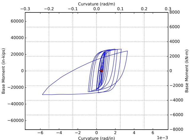
Figure N.1 Moment curvature response of model 4a for EQ1. Red circle

(29)

Figure O.1 Moment curvature response of model 4b for EQ1. Red circle

Figure P.1 Moment curvature response of model 4c for EQ1. Red circle

(30)

Figure Q.1 Moment curvature response of model 4d for EQ1. Red circle

(31)

Figure R.1 Moment curvature response of model 5a for EQ1. Red circle

Figure S.1 Moment curvature response of model 5b for EQ1. Red circle

(32)

Figure T.1 Moment curvature response of model 5c for EQ1. Red circle

(33)

Figure U.1 Moment curvature response of model 5d for EQ1. Red circle

Figure V.1 Moment curvature response of column from PEER experiment

(EQ1) [2] . . . 271

(EQ2) [2] . . . 272

(EQ3) [2] . . . 272

(EQ4) [2] . . . 273

(EQ5) [2] . . . 273

(34)

(EQ7) [2] . . . 274

(EQ8) [2] . . . 275

(35)

Chapter 1 Background

1.1 Variability in Structural Models

In the world of structural engineering, there are a number of different analytical tools

that an engineer could use to analyze a particular problem. These tools include:

simple hand calculations combined with engineering judgment, vigorous hand

cal-culations, open source software, and commercial software. Ideally, each method of

analyzing the same problem would generate the same results - or at least similar

results. However, often the case is that different analysis techniques present

differ-ent results. Further complicating the matter is the fact that even the same analysis

software can return different results based on how the particular problem is modeled.

This inherent variability of structural models can be described as uncertainty in the

models. The hypothesis behind this work is that a structural engineer can perform

an estimate of this uncertainty by combining the results of several models of the same

problem. The scope focuses in studying the inherent variability of different structural

models and providing information for the uncertainty quantification.

A selection of models were created and analyzed with a program called openSEES

(http://opensees.berkeley.edu/). The structure modeled was a single reinforced

con-crete column, representing a bridge pier. The details of the models are described in

Chapter 2. The column was loaded with gravity loads and a dynamic time history

loading taken from a series of recorded seismic events. The results from these models

(36)

test of the same column using the same dynamic time history loading. The results are

presented in Chapter 3. Finally, in Chapter 4, some thoughts are presented regarding

the resulting uncertainty from the point of view of a professional engineer.

1.2 Modeling Software

Most engineers today choose to use some sort of analysis software to model their

structure. A few of the commercial software packages that are available include:

RISA, RAM, STAAD, SAP2000, Etabs, and GTStrudl. Most commercial software is

similar in the fact that is has a graphical user interface and allows the engineer to see

their structure in 3-dimensions, apply loads, and analyze load combinations. These

software packages typically give results in the form of member stresses, deflections,

base reactions, and have a variety of different code checks that can be chosen from,

such as AISC and ACI. These programs are directly suited for structural engineers

to use for professional design purposes.

Other commercial analysis packages include finite element analysis software such

as ANSYS, Abaqus, and Solidworks simulation. The results generated from these

types of packages are typically limited to internal stresses and deformations/deflections

of the members. They may not be able to directly compare the member stresses to

the applicable building code (such as AISC or ACI).

In addition to commercial software packages, there are also many different types

of open-source software that can be used. These options typically have a much less

refined user interface than the commercial software options. Open source software

also typically has more limited functionality and may only be capable of a particular

type of analysis.

OpenSEES is a structural analysis program used by many engineers and

re-searchers worldwide to model the dynamic effects of earthquakes on structures. It is

(37)

in the 1990’s (http://opensees.berkeley.edu/). Over the years, many engineers have

developed different modeling techniques to attempt to create the most accurate

pre-diction of the real-world structural response of their particular problem. The result

is that there are now several ways to model the same problem that result in different

responses. A selection of these models was chosen for comparison.

With currently available design tools, it is not realistic to expect the time history

analysis to accurately predict the results from the shake table test. The behavior of

reinforced concrete subjected to these loads is simply too complex to predict with a

high level of certainty. Therefore, the objective of creating and analyzing models is

to get as close as possible and a "good" model is defined as a model that predicts a

response that is more accurate than other available models.

1.3 Blind Test

In addition to comparing the analysis results with each other, they were also compared

with a full scale test that was performed at the University of California, San Diego in

2010 and published by the Pacific Earthquake Engineering Research Center (PEER)

[2, 3]. In this experiment, a full scale reinforced concrete column was built on a

shake table and subjected to earthquake motions recorded during historic seismic

events. The data from this experiment is publicly available (NEES-2010-0987 from

https://www.designsafe-ci.org/data/browser/public/nees.public/ ).

The experiment was part of a blind contest performed by PEER [1]. In this

contest, engineers and researches from around the world were asked to predict the

response of the column. Figure 1.1 below shows the range of predictions that were

received for the maximum deflection at the top of the column. All contestants were

given the same information to model the column, yet the range of predicted maximum

deflections was very large. The range of predictions of the maximum moment at the

(38)

It is easy to see how the uncertainty in these models could pose a problem when the

engineer has to determine whether or not the column is adequate.

Figure 1.1: PEER contest predictions of maximum displacement at the top of column verses measured response [1]

Figure 1.2: PEER contest predictions of maximum moment at the base of the column verses measured response [1]

1.4 Related Work

Periera et al performed similar research using openSEES for numerical modeling and

(39)

uncertainty stemming solely from applying different material profiles was studied. A

total of 56 material combinations were analyzed in this work. It was found that the

accuracy of the models depended on the stress level in the column and that no single

model accurately predicted the response for the entire range of loading.

Similar work was also performed by Pan et al [5], [6], who investigated the effects

of bond slip on their fiber model of the same PEER column [2]. It was concluded that

including bond slip parameters made a substantial contribution toward the accuracy

(40)

Chapter 2 Models

2.1 General

The full scale test that the models were based on was performed at the Network for

Earthquake Engineering Simulation (NEES) shake table at the University of

Califor-nia, San Diego [2, 3]. In that experiment, a full scale bridge pier was built on the

shake table with a 522 kip concrete block on top of the pier to simulate the weight of

a bridge. The 522 kip block at the top of the pier was required to get realistic inertial

forces acting on the concrete pier. The pier itself had a round cross-section with a

diameter of 48". It was reinforced with eighteen #11 longitudinal bars and #5 hoops

spaced every 6 inches. See Figure 2.1 below. The pier was 24 feet tall, excluding the

foundation, which was 4 feet thick. The rebar was tied into the foundation to create

a moment connection and allow the pier to function as a simple cantilever column.

The mass of concrete at the top of the column was connected so that the center of

gravity of the mass was in line with the top of the column (24 feet above the top

of concrete of the footing). The connection between the pier and the superstructure

mass was designed so that there was no contact between the mass and the column

below 24 feet above TOC of the footing.

The researchers placed 250 gages and instruments onto the column prior to

test-ing [2]. The instrumentation included accelerometers on the foundation. This

ac-celerometer data was used as the input acceleration for the openSEES models. The

(41)

Figure 2.1: Pier Cross Section Details [2]

the maximum deflection that the column experienced during each of the simulated

earthquakes. This allowed the different models to not only be compared with each

other, but to be compared with the shake table response.

The software that was used for the computer analyses was the Open System for

Earthquake Engineering Simulation (openSEES). This is a software that was initially

developed by the University of California, Berkeley, and is now established as the

primary computational platform for the Pacific Earthquake Engineering Research

Center (PEER). It is an open-source platform that is used around the world for

modeling the nonlinear response of structural systems subjected to dynamic loading.

The typical process for creating a model with openSEES is the engineer downloads

a generic model from the community that resembles the system to be modeled (or

begins with a model used previously). The generic model is then modified to match

the desired dimensions, materials, conditions, etc. Right away, this presents a problem

because there are several different models that could be chosen for the same structure.

The different models range from simple, elastic analyses to advanced, nonlinear fiber

models and FEA models.

(42)

which is just about the simplest structure one would ever need to analyze. Yet, even

for this simple structure, there were several openSEES models that could be chosen

and configured for the column. And if the same column was simulated in each of the

different models, the resulting base reactions, deflections and internal stresses would

be substantially different. This difference was the inspiration behind this work.

To compare the differences between models, five commonly available models were

chosen. Table 2.1 shows the types of models used. Model 4 and model 5 each had

4 sub-models to compare different materials. Each model is discussed further in its

respective section. Once the different models were built, identical loads were applied

to each one. The acceleration load was obtained from the PEER experiment [2].

While the results of these models will be compared with the PEER test results

[2], it is important to note that no attempt was made to "fit" the models to the test

results. All of the models were created, run, and their results aggregated before being

compared with the PEER test results. There were no parameters that were adjusted

in attempt to improve the accuracy of the results. The intention was to create the

models as if no test results were available, as would be the case in a design scenario.

Table 2.1: Model Types

Model Type of Analysis No. of Elements Type of Cross-Section

Model 1 linear analysis single element solid cross-section

Model 2 linear analysis multiple elements solid cross-section

Model 3 nonlinear analysis single element solid cross-section

Model 4 nonlinear analysis single element fiber cross-section

Model 5 nonlinear analysis single element fiber cross-section

2.2 Model 1

Model 1 was the most basic model. It consisted of a single 24 foot tall element with a

16,211 slug mass at the top (applied in the model as 1.35 kip-s2_{/in to convert to the}

(43)

itself along the length (0.00043 kip-s2_{/in). This model used the elasticBeamColumn}

analysis element. This element had the limitation of a linear analysis even if the

column stress exceeded the yield stress. Table 2.2 shows the parameters used in

model 1. The primary parameter that had to be determined for this model was

the moment of inertia. A composite moment of inertia was calculated, assuming a

cracked cross-section, with all reinforcing bars intact (as opposed to selecting a state

after some bars had yielded).

Table 2.2: Parameters used for Model 1

Parameter Value

Model Name model1

Number of Elements 1

Element Type elasticBeamColumn

Fu 102 ksi

A 1810 in2

E 3320 ksi

I 97600 in4

mass 0.00043 kip-sec2

2.3 Model 2

Model 2 was similar to model 1 in most aspects except the number of elements was

increased from one to ten. This also required increasing the number of nodes from

two to eleven. This number of elements was selected after running the model with

several different numbers of elements and recording the maximum displacement in

the column. It was observed that the change in max displacement decreased as the

number of elements increased. Figure 2.2 illustrates how the maximum displacement

of the model converged once the number of elements reached approximately ten.

(44)

Model Name model2

Element Type elasticBeamColumn

Fu 102 ksi

A 1810 in2

E 3320 ksi

I 97600 in4

0 2 4 6 8 10 12 14

Number of Elements 7.60

7.65 7.70 7.75 7.80

Maximum Displacement (in)

Figure 2.2: Comparison of maximum displacement and the number of elastic elements

2.4 Model 3

Model 3 was fundamentally different from model 1 and model 2 in that it utilized

nonlinear analysis. It also used a composite material for the cross section. The

material used was “Steel01”. This material was chosen based on the assumption that

the reinforced concrete behaves in a manner similar to steel in that it has a constant

EI value up to a point and then loses stiffness and has a reduced EI beyond that point.

(45)

was one area where an approximation had to be made. Since the column had a

circular cross section, the reinforcing bars were not all a constant distance away from

the neutral axis. Therefore, all of the reinforcing bars were not expected to yield

simultaneously. Instead, as the internal moment in the column was increased, the

steel furthest from the neutral axis would reach yielding first. Then, if the moment

continued to increase, the next set of rebars would yield, and then the next, and so

on. Unfortunately, there is not an opensees material that is designed to model this

behavior explicitly. The “Steel01” material was chosen to be relatively similar to the

actual behavior (albeit simplified). The “yield” point (point at which the slope of the

moment-curvature plot abruptly changes) was determined to be 29800 in-kips based

on a moment-curvature analysis of the column.

Model Name model3

Element Type nonlinearBeamColumn

Number of Integration Points 10

f’c 6 ksi

A 1810 in2

Ec 3320 ksi

I 97600 in4

Yield Moment 29800 in-kip

Yield Curvature 0.63 x 10-4

Cracked EI 324,000,000 in2

Strain-Hardening ratio 0.04

The moment curvature plot was created by determining the moment and the

curvature associated with the first concrete crack, the yield of the most extreme

rebar, and then each subsequent rebar. The moment curvature plot is shown in

Figure 2.3. The yield point was selected as the point at which the outermost 8 rebar

(46)

0.0000 0.0001 0.0002 0.0003 0.0004 0.0005 0.0006 0.0007 0.0008 Curvature (rad/in)

0 5000 10000 15000 20000 25000 30000 35000 40000

Moment (in-kip)

Figure 2.3: Moment-Curvature of Column at Different Loading Stages

Table 2.5: Moment-Curvature Data

Stage phi M (in-kip)

No Load 0 0

1st Crack 0.0000075 7790

2 Rebar Yield 0.0000639 22500

4 Rebar Yield 0.0000689 23800

6 Rebar Yield 0.0000843 25100

8 Rebar Yield 0.0001090 27300

10 Rebar Yield 0.0001730 28900

12 Rebar Yield 0.0003780 30600

The initial EI slope was input using the cracked moment of inertia of the column

and the concrete modulus of elasticity. The cracked column moment of inertia was

taken as 97600 in4 and the modulus of elasticity was taken as 3320 ksi. The steel rebar

areas were transformed to their equivalent concrete area when calculating composite

modulii.

For the post yielding EI slope, a value of 0.04 x initial EI was used. The 0.04 value

was chosen by comparing the slopes on the moment curvature plot. The element used

in this model was ’nonlinearbeamcolumn’. Table 2.4 shows the parameters used in

(47)

2.5 Model 4

Model 4 also used the nonlinearBeamColumn element. However, the column was

modeled using a fiber cross section instead of a uniform cross section, as it was

in the previous models. There were still only two nodes and one element connecting

them. The fiber cross section was created using three materials. The interior concrete

(within the rebar cage), the exterior concrete (outside of the concrete cage), and the

longitudinal reinforcing steel. The fiber cross section was built using the ’patch’ and

’layer’ commands in openSEES. The cross section was built using 20 angular divisions

and 12 circumferential divisions, resulting in 240 total concrete fibers. Of these, 200

were within the rebar cage and 40 were outside the rebar cage.

The eighteen 36 mm (1.417 in) diameter longitudinal reinforcing bars were

mod-eled using a steel area of 1.58 square inches per bar. The material parameters: yield

strength, ultimate strength, initial modulus of elasticity, post strain hardening

mod-ulus of elasticity, strain at peak stress, and strain at initial strain hardening were

taken directly from the PEER report. These values were provided as 75.2 ksi, 102.4

ksi, 28.4 ksi, 0.8 ksi, 12.2 percent, and 1.1 percent, respectively [2], as shown in Table

2.8.

There were four different variants of model 4 that were analyzed: model4a,

model4b, model4c, and model4d. All of the models used the same concrete

ma-terial for the inner concrete layers. However, they used different concrete mama-terials

for the outer concrete layers (outside of the rebar cage). The materials are given in

(48)

Model Name model4

No. of Elements 1

No. of Integration Points 6

No. of Steel Fibers 18

No. of Interior Conc. Fibers (Radial Direction) 10

No. of Interior Conc. Fibers (Circumf. Direction) 20

No. of Exterior Conc. Fibers (Radial Direction) 2

No. of Exterior Conc. Fibers (Circumf. Direction) 20

Area of Steel Fibers 1.58 in 2

Table 2.7: Model 4 and Model 5 materials

Model Inner Concrete Outer Concrete Reinforcing Steel

4a concrete01 concrete01 ReinforcingSteel

4b concrete01 concrete02 ReinforcingSteel

4c concrete01 concrete03 ReinforcingSteel

4d concrete01 concrete04 ReinforcingSteel

5a concrete01 concrete01 ReinforcingSteel

5b concrete01 concrete02 ReinforcingSteel

5c concrete01 concrete03 ReinforcingSteel

(49)

Table 2.8: Parameters used for fiber materials in model 4 and model 5

Parameter concrete01 concrete02 concrete03 concrete04 reinforcingSteel

fpc -6 ksi -6 ksi -6 ksi -6 ksi n/a

epsc0 -0.0026 -0.0026 -0.0026 -0.0026 n/a

fpcu 0 0 0 n/a n/a

epsU -0.005 -0.005 -0.005 -0.005 n/a

lambda n/a 0.25 0.25 n/a n/a

ft n/a 0.580 ksi 0.580 ksi 0.580 ksi n/a

Ets n/a 733 ksi n/a n/a n/a

epst0 n/a n/a 0.00066 n/a n/a

ft0 n/a n/a 0.193 ksi n/a n/a

beta n/a n/a -1 n/a n/a

epstu n/a n/a 0.0021 n/a n/a

Ec n/a n/a n/a 3320 ksi n/a

fct n/a n/a n/a 0.0002 n/a

et n/a n/a n/a 0.1 n/a

Fy n/a n/a n/a n/a 75.2 ksi

Fu n/a n/a n/a n/a 102.2 ksi

Es n/a n/a n/a n/a 28400

Esh n/a n/a n/a n/a 800

esh n/a n/a n/a n/a 1.1

eult n/a n/a n/a n/a 12.2

(50)

2.6 Concrete Materials

The material concrete01 considers the concrete to have zero tensile strength (see

Figure 2.4).

Figure 2.4: Concrete01 (Source: OpenSees documentation)

The concrete02 and concrete03 materials include parameters for the concrete

ten-sile strength (see Figures 2.5 and 2.6). Concrete02 considers linear tension softening

(based on the work of Yassin et al [7]) while concrete03 considers nonlinear tension

softening.

The material concrete04 also considers concrete tensile strength with nonlinear

tension softening, using the Popovics concrete model [8] (see Figure 2.7).

2.7 Model 5

Model 5 was a fiber model similar to model 4 except that it included parameters for

strain penetration into the footing. The openSEES Bond-SP01 material was used to

model this strain penetration. A zero length element at the column base was created

(51)

slip of the rebar in the column in the area where the reinforcing bars have not yet

developed their full bond.

The parameters required for the Bond-SP01 material were: rebar yield strength

(Fy), rebar slip under yield stress (Sy), rebar ultimate strength (Fu), rebar slip at

ultimate strength (Su), initial hardening ratio (b), and pinching factor for the cyclic

slip vs bar response (R). The parameter values are shown in Table 2.10.

The slip at yield stress, Sy, was calculated by the following equation taken from

the opensees Bond-SP01 documentation, which is based on the work of Zhao and

Sritharan [9].

Sy = 0.1∗qa

db/4000∗F y/√f0_c_∗₍₂_a_{+ 1) + 0}_.₀₁₃

(52)

reinforcing steel, and f‘c is the compressive strength of the concrete. The variable ’a’

was taken as 0.4, per the CEB-FIB Model Code 90 [10]

The slip at ultimate stress was taken as 40 times the slip at yield [9], [11]. A range

for typical initial hardening ratios, b, was given in the opensees documentation as 0.3

(53)

Model Name model5

No. of Elements 1

No. of Integration Points 6

No. of Steel Fibers 18

No. of Interior Conc. Fibers (Radial Direction) 10

No. of Interior Conc. Fibers (Circumf. Direction) 20

No. of Exterior Conc. Fibers (Radial Direction) 2

No. of Exterior Conc. Fibers (Circumf. Direction) 20

Area of Steel Fibers 1.58 in 2

Table 2.10: Parameters used for Bond-SP01 material

Fy 75 ksi

Fu 102 ksi

Sy 0.04 in

Su 1.6 in

b 0.4

R 0.7

pinching factors, R, was given in the opensees documentation as 0.5 - 1.0. The value

used in model 5 was 0.7.

2.8 Number of Integration Points

It should be noted that the number of integration points was not held constant among

the different concrete models. It would be ideal for this parameter to be constant, in

order to have a better direct comparison of the different models’ results. However,

these models were very sensitive to this parameter and some of them would not

converge unless a particular number of integration points was chosen.

The maximum number of integration points that the models were capable of

(54)

used. Each model was initially run with 10 integration points. If the model failed to

(55)

Chapter 3 Results

3.1 Excitation

The excitation input files for the openSEES models were obtained from

Design-Safe (https://www.designsafe-ci.org/data/browser/public/nees.public/

NEES-2010-0987). The original experiment subjected the column to ten simulated earthquakes.

The first nine were used in the openSEES models. The tenth was omitted because

the column reached failure and hit the support structure.

The earthquake time histories were taken from two historical events: the 1989

earthquake in northern California near Loma Prieta and the 1995 earthquake in

Kobe, Japan. Three different recordings of the Loma Prieta earthquake were taken

from different monitoring stations in the San Francisco area. EQ1 was taken from

the Agnew State Hospital station. The Corralitos Station record was used for EQ2

and again for EQ4. EQ3 and EQ6 were taken from the LGPC Station. Only one

recording of the Kobe earthquake was used, but different scale factors were applied to

create increasing amplitudes for the later excitations. EQ5 used the Kobe earthquake

with a -0.8 scale factor. The scale factors for EQ7, EQ8, and EQ9 were +1.0, -1.2,

and +1.2.

In the PEER experiment[2] , the same column was used for each of the earthquake

simulations with no repairs being performed between excitations. This resulted in

accumulated damage affecting the performance of the column for each subsequent

(56)

EQ4 and EQ2 as well as the results of EQ6 and EQ3 and is discussed later in this

chapter. Each of these excitation pairs used the same time history input but had

notably different responses.

The accumulated damage was accounted for in the openSEES simulations by

linking all of the excitations into a single input file and analyzing them in a single

run. Each excitation was separated by enough time to allow all motion in the column

to dissipate. The dead time between excitations was around 120-200 seconds between

each earthquake. For comparison, each excitation was around 40 seconds in duration.

While this differed from the actual experiment that spanned two days, it was not

expected that the shortened dead time between excitations would affect the models.

The following sections describe the behavior of the models in terms of the base

shear, base moment, and top deflection. The results from the PEER experiment were

taken from [1].

The complete set of outputs from the openSEES models is included in the

appen-dices. This includes the time history response of the deflection, base shear, and base

moment of the column for each earthquake and each model.

3.2 Linear Elastic vs Nonlinear Models

Figures 3.1, 3.2, and 3.3 show the maximum shear force, bending moment and

de-flection for all models. Models 1 and 2 assumed linear elastic behavior, regardless

of the stress in the column. This resulted in extremely large base shears and

mo-ments for the later earthquakes. These results were expected, as the excitations in

the experimental test were chosen to ensure that the stresses in the column exceeded

the linear stress range. The maximum deflections of the linear elastic models were

also over-predicted, though not by as much of a margin as the base reactions. Even

though the linear elastic models resulted in unrealistically high base reactions, they

(57)

maximum values expected. This is, if other models give higher results, then it could

be an indication of an error in the non-linear models.

EQ1 Loma Prieta Agnew State Hospital Station _{EQ2 Loma Prieta Corralitos Station} EQ3 Loma Prieta LGPC Station _{EQ4 Loma Prieta Corralitos Station}

EQ5 Kobe Scale: -0.8 EQ6 Loma Prieta LGPC Station

EQ7 Kobe Scale: 1.0 _{EQ8 Kobe Scale: -1.2} EQ9 Kobe Scale: 1.2

Earthquake 0 200 400 600 800 1000 1200 1400 1600 1800

Max Base Shear (kip)

Model

1

2

3 4a

4b

4c

4d

5a

5b

5c

5d

Experiment

Figure 3.1: Maximum base shear of all models

Models 1 and 2 are linear models with the same type of element but different

number of elements. Model 1 has only 1 beam element while model 2 has 10 elements.

Figure 3.4 shows the time domain response of both models for EQ1 (Loma Prieta

- Agnew State Hospital Station). As observed in this figure, the responses are very

similar, with model 1 generally resulting in higher displacements throughout the

excitation. Figure 3.5 shows the time domain response of both models for EQ5 (Kobe

- scale -0.8). As observed in this figure, the responses are also similar, but model 2

generally resulted in higher displacements, except for the peak. Interestingly, model

1 still returned a higher peak displacement. Overall, based on the metrics defined

by the blind test competition [1] it was observed that both models have very similar

behavior, indicating that increasing the discretization to 10 elements did not make a

(58)

EQ1 Loma Prieta Agnew State Hospital Station _{EQ2 Loma Prieta Corralitos Station} EQ3 Loma Prieta LGPC Station _{EQ4 Loma Prieta Corralitos Station} EQ5 Kobe Scale: -0.8

EQ6 Loma Prieta LGPC Station

Earthquake 0 100000 200000 300000 400000 500000

Max Base Moment (in-kip)

Model

1

2

3 4a

4b

4c

4d

5a

5b

5c

5d

Experiment

Figure 3.2: Maximum base moment of all models

Because of the high values of base shear, base moment and deflection from the

linear models, it is easier to compare the results of the other models with each other

if the model 1 and model 2 results are removed. Once the linear elastic models

are removed, most of the models under-predict the base reactions. There are only

three cases where the non linear models did not under-predict the base reactions:

the maximum base shear and maximum base moment resulting from EQ4 and the

maximum base moment resulting from EQ8. Of these, the base moment resulting

from EQ 8 was only over-predicted by model 3. The fiber models (4 and 5) all

under-predicted this reaction.

(59)

EQ1 Loma Prieta Agnew State Hospital Station _{EQ2 Loma Prieta Corralitos Station} EQ3 Loma Prieta LGPC Station _{EQ4 Loma Prieta Corralitos Station}

EQ5 Kobe Scale: -0.8

EQ6 Loma Prieta LGPC Station

Earthquake 0 5 10 15 20 25 30 35 40 45 Displacement (in) Model

1

2

3 4a

4b

4c

4d

5a

5b

5c

5d

Experiment

Figure 3.3: Maximum deflection of all models

0 20 40 60 80 100 120 140 160 Time (s) 3 2 1 0 1 2 3

EQ1 Displacement (in)

(60)

780 800 820 840 860 880 900 920 Time (s)

30 20 10 0 10 20 30

EQ5 Displacement (in)

How to Make a Mudsparkler

University of South Carolina

Scholar Commons

Multi-Model Structural Analysis

Wesley Holt

Acknowledgments

Abstract

Table of Contents

List of Tables

List of Figures

Chapter 1

Background

Chapter 2

Models

Chapter 3

Results

1

2

3

4a

4b

4c

4d

5a

5b

5c

5d

Experiment

1

2

3

4a

4b

4c

4d

5a

5b

5c

5d

Experiment

1

2

3

4a

4b

4c

4d

5a

5b

5c

5d

Experiment