GROSS NON-NORMALITY AND THE QUALITY OF A SIMPLE APPROXIMATION
TO THE P-VALUE OF A ROUTINE TEST OF NON-NESTED REGRESSIONS
Jerzy Szroeter
UCL Economics Discussion Paper 1998-5
Key Words and Phrases: non-nested regressions, p-value, size, non-normality, point approximation, eigenvalues.
JEL Classification: C1, C2, C4.
ABSTRACT
1. INTRODUCTION
2
Suppose an observable random n-vector y is ascribed an N(µ, σ I )
n
distribution subject to the competing non-nested hypotheses
H : µ = Xβ versus H : µ = Zγ
0 1
where β , γ denote parameter vectors of dimensions k , g and X , Z denote observable nonrandom matrices such that rank[X] = k , rank[Z] = g , rank[X, Z] = r with n > r > max{k, g} .
It has been shown by Szroeter (1996) that the critical region for
2
the most powerful test of H versus H applicable when β, γ, σ are
0 1
2
of specified value turns into the following region when β, γ, σ are unknown and replaced by least squares estimates :
^
Q > C (1.1)
where C is an appropriate constant and
^ ^2 ^ ^ -1/2 ^
Q ≡ [σ (γ′Z′M Zγ)] [γ′Z′M y] , (1.2)
X X
^ -1
γ ≡ (Z′Z) Z′y , (1.3)
M ≡ I - S[X] , (1.4)
X n
^2
σ ≡ y′{I - S[X,Z]}y/(n - r) , (1.5)
n
where S[A] denotes the orthogonal projection operator onto the space ^ ^ spanned by the columns of matrix or matrices A . The value of σQ is equal to the routinely-computed least squares estimate of the scalar ν in the artificial regression model
^
^
The statistic Q itself only differs from the Davidson-Mackinnon (1981) ^2
J statistic in small detail : In the formula (1.5) for σ , the J ^
statistic uses [X,Zγ] and (k + 1) instead of [X,Z] and r . For connections with the Cox (1961, 1962) statistic, see McAleer (1987).
A characterization of the unknown exact finite-sample distribution ^
of Q has been obtained by Szroeter (1996). The shape and structure of that distribution depends critically on certain eigenvalues to such an extent that location-scale adjustments (see Godfrey and Pesaran (1983))
^
need not in general reduce Q to reliably approximate normal or Student T form. More fundamental adjustments to the components of the statistic may lead to undesirable side-effects. For example, the Fisher-McAleer (1981) and Godfrey (1983) adjustment based on Atkinson (1970) gives an exact test whose power function cuts below size (see Szroeter (1995)).
^
We therefore focus our research here on the unadjusted form of Q . Of particular concern are tail-probability approximations of the following type based on Szroeter’s (1996) characterization :
^
Pr{ Q > C } =
______ ______ r-k 2
(1 - λ)Pr{ T > C } + λPr{ F > C /(r - k) } (1.6)
n-r n-r
r-k
where T , F denote Student T , F variates and
n-r n-r
______ -1
λ = trace{(Z′Z) Z′M Z}/(r - k) . (1.7)
X
2. BOUNDS ON TRUE FINITE-SAMPLE SIZE
Let H (⋅) , h (⋅) denote the cdf , pdf respectively of a central
b b
chi-squared variate with b degrees of freedom. Let Φ(⋅) , φ(⋅) be
a
the cdf , pdf of a unit normal variate. Let F (⋅) denote the cdf of
b
a central F variate having a , b numerator , denominator degrees of freedom. Let the scalar m be defined as
m ≡ n - r . (2.1)
Define the function S(C,ε,ψ) on 0 < C, 0 < ε < 1, 0 < ψ < 1 as ∞ ∞
i i -1/2 -1/2 1/2
S(C,ε,ψ) ≡ 1 - j j h (w)h (τ)Φ[(1 - ψ) m W C
m r-k
0 0
-1/2 1/2 1/2
- (1 - ε) ε τ ]dτdw . (2.2)
Define the function R(C,ε,ψ) on 0 < C, 0 < ε ≤ 1, 0 < ψ ≤ 1 as
R(C,ε,ψ) ≡
∞ & L(ψ)
i i -1 -1/2 1/2 1/2 2
1 - j h (w){ φ(u)H (ε [m w C - (1 - ψ) u] )du
m j r-k
0 7 0
0 *
i -1 -1/2 1/2 1/2 2
+ j φ(u)H (ε [m w C - (1 - ε) u] )du}dw (2.3)
r-k
-∞ 8
where
-1 1/2
L(ψ) = {[(1 - ψ)m] w} C if ψ < 1 ,
L(ψ) = ∞ otherwise . (2.4)
Define
Now let λ ≤ λ ≤ ... ≤ λ denote the (possibly repeated) nonzero
d d+1 g
-1
eigenvalues of the matrix product (Z′Z) Z′M Z .
X
Following Lehmann (1986, p.69), the size α(C) of critical region (1.1) is defined as
^
α(C) ≡ sup Pr{ Q > C } (2.6)
2 k 2
where the supremum is taken over the set { (β, σ) : β ∈ R , σ > 0 }. Test p-value is the size function α(C), C ∈ R, evaluated at the point
^
C = q where q is the realized value of the variate Q . The results which follow give integral upper and lower bounds for α(C) .
THEOREM 1 : For λ < 1 , S(C,λ,λ ) ≤ α(C) ≤ S(C,λ ,λ ) .
g d g g d
THEOREM 2 : For λ ≤ 1 , R(C,λ ,λ ) ≤ α(C) ≤ R(C,λ ,λ) .
g d g g d
r -k 2
COROLLARY : For λ = 1, λ = 1 , α(C) = 1 - F [C /(r - k)] .
g d m
3. PROOFS
The proofs of Theorems 1 and 2 depend on the following Lemma which is a special case of Theorem 1 of Szroeter (1996, p.11) :
LEMMA 1 : Let U {s = 1, 2, ..., (g + 1)} be independent unit normal
s
g -1/2 g
# 2 $ # $
B ≡ 3 ∑ λ(U + θ) ∑ λ(U + θ)U , (3.1)
s s s 4 3 s s s s 4
s = d s = d
g -1 g
# 2 $ # 2 2 $
D ≡ 3 ∑ λ(U + θ) ∑ λ (U + θ) , (3.2)
s s s 4 3 s s s 4
s = d s = d
-1
where θ ≡ σ p′Z′Xβ for a right-hand eigenvector p associated with
s s s
-1
the eigenvalue λ of the matrix (Z′Z) Z′M Z , given normalization
s X
conditions p′Z′Zp = 1, p′Z′Zp = 0 for s ≠ t. Then, under H ,
s s s t 0
^
the exact finite-sample distribution of the statistic Q defined by equation (1.2) is the same as the distribution of
* 1/2 -1/2 1/2
Q ≡ m W [B + (1 - D) U ] . (3.3)
g+1
We are now in a position to prove Theorems 1 and 2.
PROOF OF THEOREM 1 :
From (3.1) we obtain the inequality
g 1/2 g 1/2
# 2 $ 1/2# 2 $
B ≤ 3 ∑ λU ≤ λ ∑ U . (3.4)
s s 4 g 3 s 4
s = d s = d
Using (3.3) and (3.4) we find that
*
Pr{ Q > C } ≤
g 1/2
1/2# 2 $ 1/2 -1/2 1/2
Pr{ [λ ∑ U + (1 - D) U ] > m W C } =
g 3 s 4 g+1
s = d
g 1/2
1/2# 2 $ 1/2 -1/2 1/2
1 - Pr{ [λ ∑ U + (1 - D) U ] ≤ m W C }. (3.5)
g 3 s 4 g+1
Now observe from (3.2) that
0 < λ ≤ D ≤ λ < 1 . (3.6)
d g
Given (3.6), we see that from (3.5) that
*
Pr{ Q > C } ≤
g 1/2
-1/2 -1/2 1/2 1/2# 2 $
1 - Pr{U ≤ (1 - D) (m W C - λ ∑ U )} ≤
g+1 g 3 s 4
s = d
g 1/2
-1/2 -1/2 1/2 -1/2 1/2# 2 $
1 - Pr{U ≤ (1 - λ ) m W C - (1 - λ ) λ ∑ U )}
g+1 d g g 3 s 4
s = d
= S(C,λ ,λ ) (3.7)
g d
where the function S(⋅) is defined by (2.2). Expression (3.7) is an *
upper bound on the probability Pr{Q > C} for each value of (β, σ), hence is an upper bound on α(C) as defined by (2.6).
The basic lower bound on α(C) is (3.7) with λ and λ
inter-d g
changed. The justification, however, differs from that for the upper bound. By (2.6) and Lemma 1,
1/2 -1/2 * * 1/2
α(C) ≥ Pr{ m W [B + (1 - D ) U ] > C } (3.8)
g+1
where
g 1/2 g 1/2
* # 2 $ 1/2# 2 $
B ≡ 3 ∑ λU ≥ λ ∑ U , (3.9)
s s 4 d 3 s 4
s = d s = d
g -1 g
* # 2 $ # 2 2 $
D ≡ 3 ∑ λU ∑ λ U , (3.10)
s s 4 3 s s 4
s = d s = d
*
g 1/2
* -1/2 -1/2 1/2 1/2# 2 $
α(C) ≥ 1 - Pr{ U ≤ (1 - D ) (m W C - λ ∑ U )}
g+1 d 3 s 4
s = d -1/2 -1/2 1/2
≥ 1 - Pr{ U ≤ (1 - λ ) m W C
-g+1 g
g 1/2
-1/2 1/2# 2 $
(1 - λ ) λ ∑ U )}
d d 3 s 4
s = d
= S(C,λ ,λ ) .
d g P
PROOF OF THEOREM 2 :
Given (3.2), observe that
g 1/2
1/2# 2 $ 1/2 -1/2 1/2
Pr{ [λ ∑ U + (1 - D) U ] ≤ m W C } ≥
g 3 s 4 g+1
s = d
g 1/2
# 2 $ -1/2 1/2 -1/2 -1/2 1/2
Pr{ [3 ∑ U + λ (1 - λ ) U ] ≤ λ m W C ,
s 4 g d g+1 g
s = d
U > 0 } + g+1
g 1/2
# 2 $ -1/2 1/2 -1/2 -1/2 1/2
Pr{ [3 ∑ U + λ (1 - λ ) U ] ≤ λ m W C ,
s 4 g g g+1 g
s = d
U ≤ 0 }
g+1
=
∞ & L(λ )
i i d -1 -1/2 1/2 1/2 2
h (w){ φ(u)H (λ [m w C - (1 - λ ) u] )du +
j m j r-k g d
0 7 0
0 *
i φ(u)H (λ-1 -1/2 1/2 1/2 2
[m w C - (1 - λ ) u] )du}dw (3.11)
j r-k g g
where L(⋅) is the function defined by (2.4). Now, relation (3.5) of
the proof of Theorem 1 continues to hold even when the assumption that λ < 1 is relaxed to λ ≤ 1 . From (2.6), (3.5), (3.11) and Lemma 1,
g g
we then obtain the upper bound of Theorem 2 .
As for the lower bound on α(C) , equations (3.8) to (3.10) of the proof of Theorem 1 also continue to hold when the assumption λ < 1
g
is weakened to λ ≤ 1 . Therefore,
g
g 1/2
# 2 $ -1/2 * 1/2 -1/2 -1/2 1/2
α(C) ≥ Pr{ [3 ∑ U + λ (1 - D ) U ] > λ m W C ,
s 4 d g+1 d
s = d
U > 0 } + g+1
g 1/2
# 2 $ -1/2 * 1/2 -1/2 -1/2 1/2
Pr{ [3 ∑ U + λ (1 - D ) U ] > λ m W C ,
s 4 d g+1 d
s = d
U ≤ 0 }
g+1
g 1/2
# 2 $ -1/2 1/2 -1/2 -1/2 1/2
≥ Pr{ [3 ∑ U + λ (1 - λ ) U ] > λ m W C ,
s 4 d g g+1 d
s = d
U > 0 } + g+1
g 1/2
# 2 $ -1/2 1/2 -1/2 -1/2 1/2
Pr{ [3 ∑ U + λ (1 - λ ) U ] > λ m W C ,
s 4 d d g+1 d
s = d
U ≤ 0 } . (3.12)
g+1
We now note that
g 1/2
# 2 $ -1/2 1/2 -1/2 -1/2 1/2
Pr{[3 ∑ U + λ (1 - λ ) U ] ≤ λ m W C, U > 0}
s 4 d g g+1 d g+1
=
∞ & L(λ ) *
i i g -1 -1/2 1/2 1/2 2
h (w){ φ(u)H (λ [m w C - (1-λ ) u] )du}dw (3.13)
j m j r-k d g
0 7 0 8
where L(⋅) is the function defined by (2.4). Similarly,
g 1/2
# 2 $ -1/2 1/2 -1/2 -1/2 1/2
Pr{[3 ∑ U + λ (1 - λ ) U ] ≤ λ m W C, U ≤ 0}
s 4 d d g+1 d g+1
s = d
=
0 *
i φ(u)H (λ-1 -1/2 1/2 1/2 2
[m w C - (1 - λ ) u] )du}dw . (3.14)
j r-k d d
-∞ 8
Given the definition (2.3), relations (3.12), (3.13), (3.14) imply that
α(C) ≥ R(C,λ ,λ ) ,
d g
which is the lower bound of Theorem 2. P
4. NUMERICAL COMPUTATIONS AND COMPARISONS
By Theorems 1 and 2,
α(C) = S(C,λ,λ) = R(C,λ,λ) for λ = λ = λ < 1 , (4.1)
d g
(r - k) > 2, double integration cannot be avoided but, when (r - k) = 2, R(C,λ,λ) can be rewritten in the single integral form
∞ &
i -1/2 -1/2 1/2
R(C,λ,λ) = 1 - j h (w){ Φ[(1 - λ) m W C]
-m
0 7
*
1/2 2 1/2 -1/2 -1/2 1/2
λ exp[-wC /(2m)]Φ[λ (1 - λ) m W C] }dw . 8
(4.2) We therefore compute α(C) , to a numerical accuracy of ± 0.001, using α(C) = R(C,λ,λ) with R(⋅) as given by (4.2) for (r - k) = 2, but using α(C) = S(C,λ,λ) with S(⋅) as given by (2.2) for (r - k) = 4, 8 . This This is done for each λ = 0.25, 0.5, 0.75 across the range C = 1.3, 1.7, 2.1, 2.5, 2.9, 3.3, 3.7. We use the typical figure of 30 for m . Alongside each value of α(C) we place for comparison the values of
T(C) ≡ Pr{ T > C } , (4.3)
m
r -k 2
F(C) ≡ Pr{ F > C /(r - k) } , (4.4)
m
M(C) ≡ (1 - λ)T(C) + λF(C) , (4.5)
r -k
where T , F denote central Student T, F variates and M(C) is the
m m
" T, root-F mixture " approximation (1.6) described in Section 1.
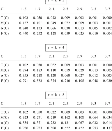
TABLE I
Comparison of Student T, Root-F and Mixture Approximations
for the Exact P-Value of a Test of Non-Nested Regressions
The Case λ = 0.25
---u---o
p p
p r = k + 2 p m---.
C 1 . 3 1 . 7 2 . 1 2 . 5 2 . 9 3 . 3 3 . 7
---T (C) 0 . 102 0 . 050 0 . 022 0 . 009 0 . 003 0 . 001 0 . 000 M(C) 0 . 187 0 . 101 0 . 049 0 . 022 0 . 009 0 . 003 0 . 001 α(C) 0 . 240 0 . 133 0 . 066 0 . 030 0 . 013 0 . 005 0 . 002 F (C) 0 . 440 0 . 252 0 . 128 0 . 059 0 . 025 0 . 010 0 . 004
u---o
p p
p r = k + 4 p m---.
C 1 . 3 1 . 7 2 . 1 2 . 5 2 . 9 3 . 3 3 . 7
---T (C) 0 . 102 0 . 050 0 . 022 0 . 009 0 . 003 0 . 001 0 . 000 M(C) 0 . 274 0 . 183 0 . 110 0 . 059 0 . 029 0 . 013 0 . 005 α(C) 0 . 355 0 . 218 0 . 120 0 . 060 0 . 027 0 . 012 0 . 005 F (C) 0 . 791 0 . 583 0 . 374 0 . 210 0 . 105 0 . 048 0 . 020
u---o
p p
p r = k + 8 p m---.
C 1 . 3 1 . 7 2 . 1 2 . 5 2 . 9 3 . 3 3 . 7
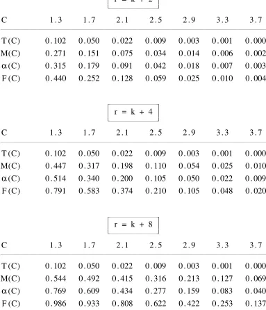
TABLE II
Comparison of Student T, Root-F and Mixture Approximations
for the Exact P-Value of a Test of Non-Nested Regressions
The Case λ = 0.5
---u---o
p p
p r = k + 2 p m---.
C 1 . 3 1 . 7 2 . 1 2 . 5 2 . 9 3 . 3 3 . 7
---T (C) 0 . 102 0 . 050 0 . 022 0 . 009 0 . 003 0 . 001 0 . 000 M(C) 0 . 271 0 . 151 0 . 075 0 . 034 0 . 014 0 . 006 0 . 002 α(C) 0 . 315 0 . 179 0 . 091 0 . 042 0 . 018 0 . 007 0 . 003 F (C) 0 . 440 0 . 252 0 . 128 0 . 059 0 . 025 0 . 010 0 . 004
u---o
p p
p r = k + 4 p m---.
C 1 . 3 1 . 7 2 . 1 2 . 5 2 . 9 3 . 3 3 . 7
---T (C) 0 . 102 0 . 050 0 . 022 0 . 009 0 . 003 0 . 001 0 . 000 M(C) 0 . 447 0 . 317 0 . 198 0 . 110 0 . 054 0 . 025 0 . 010 α(C) 0 . 514 0 . 340 0 . 200 0 . 105 0 . 050 0 . 022 0 . 009 F (C) 0 . 791 0 . 583 0 . 374 0 . 210 0 . 105 0 . 048 0 . 020
u---o
p p
p r = k + 8 p m---.
C 1 . 3 1 . 7 2 . 1 2 . 5 2 . 9 3 . 3 3 . 7
TABLE III
Comparison of Student T, Root-F and Mixture Approximations
for the Exact P-Value of a Test of Non-Nested Regressions
The Case λ = 0.75
---u---o
p p
p r = k + 2 p m---.
C 1 . 3 1 . 7 2 . 1 2 . 5 2 . 9 3 . 3 3 . 7
---T (C) 0 . 102 0 . 050 0 . 022 0 . 009 0 . 003 0 . 001 0 . 000 M(C) 0 . 356 0 . 202 0 . 102 0 . 047 0 . 020 0 . 008 0 . 003 α(C) 0 . 381 0 . 218 0 . 111 0 . 051 0 . 021 0 . 008 0 . 003 F (C) 0 . 440 0 . 252 0 . 128 0 . 059 0 . 025 0 . 010 0 . 004
u---o
p p
p r = k + 4 p m---.
C 1 . 3 1 . 7 2 . 1 2 . 5 2 . 9 3 . 3 3 . 7
---T (C) 0 . 102 0 . 050 0 . 022 0 . 009 0 . 003 0 . 001 0 . 000 M(C) 0 . 619 0 . 450 0 . 286 0 . 160 0 . 080 0 . 036 0 . 015 α(C) 0 . 657 0 . 461 0 . 284 0 . 155 0 . 076 0 . 034 0 . 015 F (C) 0 . 791 0 . 583 0 . 374 0 . 210 0 . 105 0 . 048 0 . 020
u---o
p p
p r = k + 8 p m---.
C 1 . 3 1 . 7 2 . 1 2 . 5 2 . 9 3 . 3 3 . 7
r = k + 4), 0.61 (when r = k + 8). F(C) overestimates these figures as 0.25, 0.58 and 0.93 respectively. The mixture approximation M(C) gives figures of 0.15, 0.32, and 0.50. These are undoubtedly a considerable improvement on T(C) and F(C).
In all cases, the inequality T(C) < min{ M(C), α(C) } ≤ max{ M(C), α(C) } < F(C) holds. When r = (k + 2) , the inequality M(C) ≤ α(C) holds throughout the computed range of C but, when r = (k + 8), it holds only for the lower C values of 1.3, 1.7, 2.1. It switches to M(C) > α(C) at C values of 2.5, 2.9, 3.3, 3.7. Switching also occurs for r = (k + 4) , but in that case the switch point C depends on the value of λ .
The approximation M(C) seems to be most effective at size levels from 0.2 down. For example, in the case λ = 0.25, when M(C) indicates levels of 0.10, 0.11, 0.16 for r = (k + 2), (k + 4), (k + 8) , then the true level α(C) equals 0.13, 0.12, 0.13 respectively. In the case λ = 0.50, for the same values of r, when M(C) indicates levels of 0.08, 0.11, 0.13 , then α(C) equals 0.09, 0.11, 0.08. In the final case λ = 0.75 , for the same values of r, when M(C) equals 0.10, 0.16, 0.10, then α(C) equals 0.11, 0.16, 0.08. The approximation M(C) performs less well at higher p-values than 0.2, but it remains considerably more informative than the very misleading undervaluation T(C).
BIBLIOGRAPHY
Atkinson, A.C. (1970). "A method for discriminating between models," Journal of the Royal Statistical Society B, 32, 323-353.
Cox, D.R. (1962). "Further results on tests of separate families of hy-potheses," Journal of the Royal Statistical Society B, 24, 406-424.
Davidson, R. and J.G. MacKinnon (1981). "Several tests for model spec-ification in the presence of alternative hypotheses," Econometrica, 47, 781-793.
Fisher, G.R. and M. McAleer (1981). "Alternative procedures and associ-ated tests of significance for non-nested hypotheses," Journal of Econometrics, 16, 103-119.
Godfrey, L.G. (1983). "Testing non-nested models after estimation by instrumental variables or least squares," Econometrica, 51, 355-365. Godfrey, L.G. and M.H. Pesaran (1983). "Tests of non-nested regression models: small-sample adjustments and Monte Carlo evidence," Journal of Econometrics, 21, 133-154.
Lehmann, E.L. (1986). Testing Statistical Hypotheses. New York: John Wiley & Sons.
McAleer, M (1987). "Specification tests for separate models: a survey," Specification Analysis in the Linear Model, (M. King and D. Giles, Eds.). London: Routledge & Kegan Paul, 146-195.
Szroeter, J. (1995). "The exact power function of an exact test of a regression model against multiple separate alternatives," Communic-ations in Statistics - Theory and Methods, 24, 2329-2339.