A Method of Solving Compressible Navier Stokes
Equations in Cylindrical Coordinates Using
Geometric Algebra
Terry E. Moschandreou1,2,*
1 London International Academy, 365 Richmond Street London, ON, N6A 3C2, Canada;
2 Department of Applied Mathematics, Faculty of Science, Western University, London Ontario, N6A 5C1,
Canada
* Correspondence:[email protected]@uwo.ca;Tel.:+1-519-452-4430
Abstract 1
A method of solution to solve the compressible unsteady 3D Navier-Stokes Equations in 2
cylindrical co-ordinates coupled to the continuity equation in cylindrical coordinates is presented in 3
terms of an additive solution of the three principle directions in the radial, azimuthal and z directions 4
of flow. A dimensionless parameter is introduced whereby in the large limit case a method of solution 5
is sought for in the boundary layer of the tube. A reduction to a single partial differential equation is 6
possible and integral calculus methods are applied for the case of a body force directed to the centre 7
of the tube to obtain an integral form of the Hunter-Saxton equation. Also an extension for a more 8
general body force is shown where in addition there is a rotational force applied. 9
1. Introduction 10
Compressible flow has many applications some of which are of physics, mathematics and 11
engineering interest. In general we have two types of flows, internal and external. Internal flows in 12
ducts are important in industry and nozzles and diffusers used in engines are also an applied area for 13
these types of flows. In general, density changes are related to temperature changes. External flows 14
can be important for airplanes and projectiles where compressiblilty effects are important. The Navier 15
Stokes equations have been dealt with extensively in the literature for both analytical [8] and numerical 16
solutions [9], [3]. Some work converting the compressible Navier-Stokes equations to the Schrödinger 17
equation in quantum mechanics by means of transformations has been carried out by Vadasz. [10]. 18
General mathematical and computational methods for compressible flow have been outlined in [6]. 19
Methods in more general fluid mechanics are also addressed in [1]. In the context of functional analysis 20
it has been shown in [5] that generally the motion of a compressible fluid with fixed initial velocity 21
field and constant initial density converges to that of an incompressible fluid as it’s sound speed goes 22
to infinity. Some analytical methods such as in [2] have been successfully carried out for one and two 23
dimensional isentropic unsteady compressible flow. Little is known though for analytical methods 24
for three dimensional compressible unsteady flow for both isentropic and non-isentropic flow. In the 25
present work I introduce a new procedure to write the compressible unsteady Navier Stokes equations 26
with a general spatial and temporal varying density term in terms of an additive solution of the three 27
principle directions in the radial, azimuthal andzdirections of flow. A dimensionless parameter is 28
introduced whereby in the large limit case a method of solution is sought for in the boundary layer 29
of the tube. It is concluded that the total divergence of the flow can be expressed as the integral with 30
respect to time of the line integral of the dot product of inertial and azimuthal velocity. The line 31
integral is evaluated on a contour that is annular and traces the boundary layer as time increases in the 32
flow. A reduction to a single partial differential equation is possible and integral calculus methods are 33
applied for the case of a body force directed to the centre of the tube to obtain an integral form of the 34
Hunter-Saxton equation. Also an extension for a more general body force is shown where in addition 35
there is a rotational force applied. 36
2. A new composite velocity formulation 37
The 3D compressible cylindrical unsteady Navier-Stokes equations are written in expanded form, for each component,ur,uθanduz:
∂ur ∂t +ur
∂ur ∂r +
uθ
r
∂ur
∂θ −
u2θ r +uz
∂ur ∂z −
µ
ρ −
ur
r2 +
∂2ur ∂r2 +
1 r
∂ur ∂r +
1 r2
∂2ur ∂θ2 −
2 r2
∂uθ
∂θ +
∂2ur ∂z2
!
−
µ
3ρ ∂
∂r ∂ur
∂r +
1 r
∂ur
∂θ +
∂ur ∂z
! + 1
ρ ∂p
∂r −Fgr =0 (1)
∂uθ ∂t +ur
∂uθ ∂r +
uθ
r
∂uθ
∂θ +
1
ruruθ+uz
∂uθ ∂z −
µ
ρ −
uθ
r2 +
∂2uθ ∂r2 +
1 r
∂uθ ∂r +
1 r2
∂2uθ ∂θ2 +
2 r2
∂ur
∂θ +
∂2uθ ∂z2
!
−
1 r
µ
3ρ ∂
∂θ ∂uθ
∂r +
1 r
∂uθ
∂θ +
∂uθ ∂z
! + 1
ρr ∂p
∂θ −Fgθ=0 (2)
∂uz ∂t +ur
∂uz ∂r +
uθ
r
∂uz ∂θ +uz
∂uz ∂z −
µ
ρ ∂2uz
∂r2 +
1 r
∂uz ∂r +
1 r2
∂2uz ∂θ2 +
∂2uz ∂z2
!
−
µ
3ρ ∂
∂z ∂uz
∂r +
1 r
∂uz
∂θ +
∂uz ∂z
! + 1
ρ ∂p
∂z −Fgz=0 (3)
whereur is the radial component of velocity,uθis the azimuthal component anduz is the velocity
component in the direction along tube,ρis density, µis dynamic viscosity ,Fgr,Fgθ,Fgzare body
forces on fluid. The total gravity force vector is expressed asF~T= (Fgr,Fgθ,Fgz).
The following relationships between starred and non-starred dimensional quantities together with a non-dimensional quantityδare used:
ur = 1 δ2u
∗
r (4)
uθ = 1
δu ∗
θ (5)
uz= 1 δu
∗
z (6)
r= r ∗
δ (7)
z= 1
δz
∗,t=t∗ (9)
whereδ = r1∗∂θ∂ρ∗
∂ρ ∂r∗+
ρ
r∗ −1
as part of the continuity equation (Eq(12)). The region of interest is confined to within the boundary layer which is created in an assumed compressible viscous flow in the tube. Using Eqs.(4-9),multiplying Eqs(1-3) by cartesian unit vectorse~r∗ = (1, 0, 0),e~
θ∗ = (0, 1, 0)
and~k= (0, 0, 1)respectively and adding Equations (1-3) gives the following equation, for the resulting composite vectorL1~ = 1
δ2u
∗ r∗e~r∗+1
δu
∗
θ∗e~θ∗+1δu
∗ z∗~k,
δ
1
δ ∂L~1
∂t∗ +
u∗r∗
δ2 ∂L~1
∂r∗ +
u∗θ∗
δr∗ ∂L~1
∂θ∗ +
1
δu ∗ z∗∂
~
L1
∂z∗ −
1
δ2r∗u ∗2
θ∗e~r∗+
1
δ3r∗u ∗ r∗u∗θ∗e~θ∗
− µ ρ −δ
2L1~ r∗2+δ
2∂2L1~
∂r∗2
+δ21
r∗ ∂L1~ ∂r∗ +δ
2 1 r∗2
∂2L1~ ∂θ∗2
+2δ 2 r∗2
1
δ2 ∂ur∗∗
∂θ∗ e~θ
∗−1
δ ∂u∗θ∗
∂θ∗ e~r
∗
+δ2
∂2L1~ ∂z∗2
− µ 3ρ ∂
∂r∗ ∂u∗r∗
∂r∗ +
1 r∗
∂u∗r∗
∂θ∗ + ∂u∗r∗
∂z∗
!
~
er∗− δ r∗ µ 3ρ ∂ ∂θ∗ ∂u∗θ∗
∂r∗ +
1 r∗
∂u∗θ∗
∂θ∗ + ∂u∗θ∗
∂z∗
!
~
eθ∗
−δµ
3ρ ∂
∂z∗ ∂u∗z∗
∂r∗ +
1 r∗
∂u∗z∗
∂θ∗ + ∂u∗z∗
∂z∗
!
~k+δ1 ρ
∂p ∂r∗e~r
∗+δ 1 r∗ρ
∂p ∂θ∗e~θ
∗+δ1 ρ
∂p ∂z∗
~k−F~T=0 (10)
Furthermore one can take the cross product of Equation (10) with e~r∗ and e~θ∗ to form two equations respectively where in the second case multiplication byδ to cancel squared nonlinear
terms,− 1
δ2r∗u
∗2
θ∗e~r∗,
1
δ3r∗u
∗
r∗u∗θ∗e~θ∗, leads to,
δ 1
δ ∂L~A
∂t∗ +
u∗r∗
δ2 ∂L~A
∂r∗ +
u∗θ∗
δr∗ ∂L~A
∂θ∗ +
1
δu ∗ z∗∂
~
LA ∂z∗
!
+δ−2u ∗
θ∗
r∗
−ρL−∂ρ∂t−u∗z∗∂ρ
∂z∗ ∂ρ
∂r∗
~k−
µ
ρ
−δ
2L~A
r∗2 +δ 2∂2L~A
∂r∗2
+δ21
r∗
∂L~A ∂r∗ +δ
2 1 r∗2
∂2L~A ∂θ∗2
+2δ 2 r∗2
1
δ2 ∂ur∗∗
∂θ∗ ~k−1
δ ∂u∗θ∗
∂θ∗ ~k
+δ2
∂2L~A ∂z∗2
+ +δ r∗ µ 3ρ ∂ ∂θ∗ ∂u∗θ∗
∂r∗ +
1 r∗
∂u∗θ∗
∂θ∗ + ∂u∗θ∗
∂z∗
!
~k+δµ
3ρ ∂
∂z∗ ∂u∗z∗
∂r∗ +
1 r∗
∂u∗z∗
∂θ∗ + ∂u∗z∗
∂z∗
!
~
eθ∗−
δµ
3ρ ∂
∂r∗ ∂u∗r∗
∂r∗ +
1 r∗
∂u∗r∗
∂θ∗ + ∂u∗r∗
∂z∗
!
~k+δ2µ 3ρ
∂
∂z∗ ∂u∗z∗
∂r∗ +
1 r∗
∂u∗z∗
∂θ∗ + ∂u∗z∗
∂z∗
!
~
er∗−δ 1
r∗ρ ∂p ∂θ∗
~k−
δ1 ρ
∂p ∂z∗e~θ
∗+δ21 ρ
∂p ∂r∗
~k−δ21
ρ ∂p ∂z∗e~r
∗+F~T=0 (11)
38
where L~A = −u∗z∗e~r∗−1
δu
∗ z∗~e∗
θ +
1
δ(u
∗
r∗−u∗θ∗)~k, L~A = L1~ ×e~r∗+δL1~ ×~e∗
θ and continuity equation,
39
Eq(12) below has been used. Equation (10) is sufficient to carry out the subsequent analysis. 40
41
3. A Solution Procedure forδarbitrarily large in quantity
42
Multiplication of Eq.(10) by ρδ and Eq.(12) below by L~1
δ , addition of the resulting equations [7],
The continuity equation in cylindrical co-ordinates is
∂ρ
∂t +
1
δu ∗ r∗ ∂ρ
∂r∗ +
u∗θ∗ r∗
∂ρ
∂θ∗ +u ∗ z∗ ∂ρ
∂z∗ =−ρ
1
δ
u∗r∗ r∗ +
1
δ ∂u∗r∗
∂r∗ +
1 r∗
∂u∗θ∗
∂θ∗ + ∂u∗z∗
∂z∗
!
=−ρL (12)
ρ∂~a
∂t +~a· ∇~a+ρ
2~b∇ ·~b=
µ(δ)
∇2~b+1
3∇(∇ ·~b)
+∇P+F~T (13)
whereµ(δ) =µδ. I denote it byµbelow.
Taking the geometric product in the previous equation with the inertial vector term,
~f =~a· ∇~a (14)
where~b=~aρis defined, where in the context of Geometric Algebra, the following scalar and vector 43
grade equations arise, 44
45
~f · ρ2∂~b
∂t +ρ ~b∂ρ
∂t
! +
~f 2
+~b·~fρ2∇ ·~b=
µ~f· ∇2~b+µ
3~f· ∇(∇ ·~b) +~f· ∇P (15)
∂~b ∂t +
1
ρ ~b∂ρ
∂t +
~bρ2∇ ·~b=µ∇2~b+1
3∇(∇ ·~b)
+∇P+F~T (16)
The geometric product of two vectors [4], is defined byA~~B=A~·~B+A~×~B.
Taking the divergence of Eq.(16) results in
∂
∂t
∇ ·~b+ 1
ρ ∂ρ
∂t∇ ·
~b+~b· ∇(1 ρ
∂ρ
∂t) +∇ ·(
~bρ2∇ ·~b) =∇ ·
µ∇2(~b
+
µ
3∇ ·
∇(∇ ·~b)+∇ ·(∇P) +∇ ·F~T (17)
Upon multiplication of Eq(17) by,
H= ρ 3~b·~f
∂ρ ∂t
(18)
the resulting equation is
H∂
∂t(∇ ·
~b) +ρ2~b·~f∇ ·~b+H~b· ∇(1 ρ
∂ρ
∂t) +H∇ ·(
~bρ2∇ ·~b) =
µH∇ · ∇2~b+µ
which results upon using Eq(15) in,
H∂
∂t(∇ ·
~b)−~f · ρ2∂~b
∂t +ρ ~b∂ρ
∂t
!
−
~f 2
−µ~f· ∇2~b−µ
3~f· ∇(∇ ·~b)−~f · ∇P+H~b· ∇( 1
ρ ∂ρ
∂t)+
H∇ ·(~bρ2∇ ·~b) =µH(∇ · ∇2~b) +µ
3H∇ ·(∇(∇ ·~b)) +H∇ ·(∇P) +H∇ ·F~T (20)
The continuity equation is written in terms of~bas,
∂ρ
∂t +ρ
2∇ ·~b+
ρ~b· ∇ρ+ρ∇ρ·~b=0 (21)
and
∇ ·~b=−1 ρ2
∂ρ
∂t −
2
ρ∇ρ·
~b (22)
where the following compact expression is given,
Y∗=∇ ·~b (23)
Multiplying by(~f·~f)−1in Eq.(20) and, using properties of third derivatives involving the gradient and in particular the fact that the Laplacian of the divergence of a vector field is equivalent to the divergence of the Laplacian of a vector field, leads to the following form,
W∗∂Y
∗
∂t −G(ρ, ∂ρ
∂t)W ∗−F(
ρ,∂ρ ∂t)
~b~f(1+~f · ∇P)−V(µ)W∗∇2(Y∗)−~b~f∂ρ ∂t
ρ−3
~f
2~f·
∂~b ∂t
! +Ω−
~b~f∂ρ ∂t
ρ−3
~f
2µ~f· ∇
2~b−~b~f∂ρ ∂t
ρ−3
~f 2
µ
3~f· ∇(∇ ·~b)−~b~f 1
~f
2~b·~f ∇ ·
~bρ2∇ ·~b+∇P+F~T=0 (24)
whereΩ=H~b· ∇(1
ρ ∂ρ
∂t)in Eq.(24) and,
W∗ =
~f ·~b
~f
2~f
~b=
~f ·~b
~f
2~f
·~b+
~f ·~b
~f
2~f
×~b=ξ+~f ×
~f ·~b
~f
2~b
(25)
This involves the vector projection of~bonto~f which is written in the conventional form,
projfb= f·b
kfk2f (26)
Equation (24) can be written compactly as
∂Y∗ ∂t −G(ρ,
∂ρ
∂t)−V(µ)∇
2Y∗− ∇2P= U~f h
Q(ρ,∂ρ∂t,~b,∂∂~bt,∇P,F~T) +~f
i
U~f~b
whereU~f~ξis the scalar projection for~b,Qand hence for a constantα,
∂Y∗ ∂t −G(ρ,
∂ρ
∂t)−V(µ)∇
2Y∗− ∇2P= Q(ρ,
∂ρ ∂t,
~b,∂~b
∂t,∇P,F~T) +
~f
~b
=α (28)
with solution in terms of a functionB,
Y∗ =∇ ·~b=B(α,r,θ,z,t) (29)
If the rate of change ofρwith respect totis changing exponentially in time as 1rB(θ,z)e−ctfor some
real constantcsuch thatO(c2)≈0,Ba general function which vanishes inG(ρ,∂ρ∂t) = (
∂ρ ∂t)2
ρ2 , and since
ρisO(1/r)in boundary layer, it may be proven thatB is written linearly in terms of a separable
function, that is
B(α,r,θ,z,t) =F1(r)F2(θ)F3(z)F4(t)−1/4
C1+C2ln(r) +C3r2 c2+α
µC3
(30)
whereFiare the separable parts of the function andCjare arbitrary constants. Also it is assumed that higher order derivatives are negligible in the boundary layer, so that the Laplacian of pressure is dropped and the gradient of pressure is preserved.
Forc2approaching zero and using the properties of the norm,
h
Y∗(r,θ,z,t)− F1(r)F2(θ)F3(z)F4(t)
i
~b−M(r)
Q ρ,
∂ρ
∂t, ~b,∂~b
∂t,∇P, ~
FT
! +~f
=0 (31)
Furthermore using the property for a norm on a vector space of continuous functions(since away from r=0) ,kAk=0 iffA=0, and Eq.(16) and the second line of Eq.(24) gives,
h
Y∗(r,θ,z,t)− F1(r)F2(θ)F3(z)F4(t)
i
~b−
K(ρ,∂ρ ∂t)M(r)
"
−2∂~b
∂t −
1
ρ ~b∂ρ
∂t −F(ρ, ∂ρ
∂t)(
~f +∇P)−~b∇ ·−~bρ2∇ ·~b+F~
T
#
=0 (32)
whereM(r)is the function on the very right side of Eq.(30).
h
∇ ·~b− F1(r)F2(θ)F3(z)F4(t)
i
~b−
K(ρ,∂ρ ∂t)M(r)
"
−2∂~b
∂t −
1
ρ ~b∂ρ
∂t −F(ρ, ∂ρ
∂t)(
~f +∇P)−~b∇ ·F~T
#
=0 (33)
whereF(ρ,∂ρ
∂t) =ρ
−3∂ρ
∂t.Ωin Eq.(24) vanishes due to assumption on rate of change of density with
respect totandc2 ≈0, and finally Eq.(22) has been used with a calculation done to show that the expression reduces in going from Eq (32) to Eq(33). This occurs in the boundary layer due to density beingO(1/r).
an increasing function radially there with the following resulting upon dividing byKandM(r), "
−2∂~b
∂t −
1
ρ ~b∂ρ
∂t −F(ρ, ∂ρ
∂t)(
~f +∇P)−~b∇ ·F~T
#
=0 (34)
Dividing byF(ρ,∂ρ∂t)and taking the curl of Eq.(34) simplifies to the following in the boundary layer,
−2F−1∂
∂t∇ ×
~b− ∇ ×~f−F−1∇ ×~b∇ ·F~T=0 (35)
The inertial vector~f =∇(f2/2)−~a× ∇ ×~a.
Multiply Eq.(35) by the normal vector cos(θ)~a which is the normal component of~a at wall of
moving control volume (CV) in Figure 1,
cos(θ)~a·
−2F−1∂
∂t∇ ×
~b− ∇ ×~f−F−1∇ ×~b∇ ·F~
T
=0 (36)
Choosingρso thatF=2 the following is used,
Recalling Divergence theorem and Stoke’s theorem, for generalF, ˚
V
(∇ ·F)dV= ‹
S(V) F· ˆndS
¨
S
(∇ ×F)·dS= ˛
C
F(r)·dr (37)
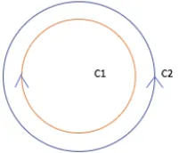
whereC=C1∪C2defines the union of two contours where the first is at the boundary layer edge and the other is along the wall (Fig. 2) andSconsists of all surfaces of control volume.
Defining the following vector field,
~
W=−∂ ∂t∇ ×
~b−1
2∇ ×
~b∇ ·F~T, (38)
‹
S(V)
W·ˆndS= ˚
V
(∇ ·W)dV (39)
= ˛
Cf
(r)·dr (40)
where ˆn=cos(θ)~a, and Stoke’s theorem has been used.
˛
C
~f(r)·~Tds=−
˛
C (∂~b
∂t +
1
where~Tis unit tangent vector to closed curveCanddsis arc length, ˛
C
(~f(r) +∂~b
∂t +
1
2~b∇ ·F~T)·dr=0 (42) The third term in the parenthesis in Eq(42) is integrated by parts for line integral and I obtain the following,
˛
C
(~f(r) +∂~b
∂t −
1
2F~T∇ ·~b)·dr=0 (43) Parametrizing the circle asr=g(θ)in polar coordinates it can be proven that the line integral in Eq(43)
is, ˛
C
(f1+ ∂b1
∂t −
1
2FT1∇ ·~b)·dθ−
˛
C
(f2+∂b2
∂t −
1
2FT2∇ ·~b)·dr=0 (44) The normal form of Green’s theorem can be used for the line integral in Eq(44),setting first,
M= f1+
∂b1 ∂t −
1
2FT1∇ ·~b (45)
N= f2+
∂b2 ∂t −
1
2FT2∇ ·~b (46)
The line integral in Eq(44) is equal to the following,
¨
R
∂M ∂r +
∂N ∂θ
drdθ (47)
whereMandNare given by Eqs(45) and (46) respectively andRis the annulus with boundaryC. The external forceFT1 is expressed as follows.(see Appendix ),
FT1 =µsin(θ)
ˆ r
rBL ∂b2
∂θ dr (48)
It follows that Eq.(47) becomes, 46
47
¨
R
µsin(θ) ˆ r
rBL ∂b2
∂θ dr
∂
∂r
1 r
∂b2 ∂θ
+µsin(θ)1
r
∂b2 ∂θ
2
+ (f2+∂b2
∂t )θ
drdθ (49) and since the boundary layer is thin the first integral vanishes and the Eq.(47) becomes,
¨
R
"
µsin(θ)1
r
∂b2 ∂θ
2
+ (f2+
∂b2 ∂t )θ
#
drdθ (50)
In the boundary layer the functionb2=b2(θ,t)andb1=b1(r,t)and thus,
ˆ 2π
0
(r−rBL)(b2b2θ+b2t)θ−µsin(θ)ln(
r rBL
)b22 θ
!
Dividing byr−rBL,forθ≈π/2, and using L’Hopital’s rule, I obtain the Hunter Saxton equation with
48
µrBL =1.
49
50
4. The Hunter-Saxton Equation 51
Substituting f2andFT1 into Eq(45) and (46) sinceFT2 =0 and f1,b1terms are negligible in the boundary layer(Recallur=u∗r/δ2,t=t∗/δthen one can obtain an integral form of the Hunter-Saxton equation using Eq.(47),
b∗2t+b2∗b∗2 θ
θ
= 1 2b
∗
2θ
2 (52)
It necessarily follows that for small θ approximation that ∂b2∂θ(0,t) = 0, ∂ 2b
2(0,t)
∂2θ = 0, and higher
52
derivatives at zero are zero. 53
54
It is of interest that a more complicated partial differential equation is manifest upon taking 55
FT2 to be non zero and thus defining a rotational force related to the vorticity of the fluid elements in
56
the boundary layer. 57
Figure 1.Compressible Viscous Flow in a Tube,zblis the distance to achieve maximum boundary layer
height.
Figure 2.A Typical set of contour lines between edge of boundary layer and tube wall. 58
In the interval[0,t]the boundary layer starts to form att=0 and reaches maximum height at timet. 59
See Fig. 1 for control volume over the growth of the boundary layer. The time dependence is shown in 60
the inertial term~f. The right side of Eq.(40) consists of nonlinear inertial term~f and Eq.(39) shows the 61
dependence on these gradients and rate of change of curl of~bwith respect tot. 62
5. Conclusion 63
An attempt has been made to reduce the compressible Navier Stokes equations coupled to the 64
continuity equation in cylindrical co-ordinates to a simpler problem in terms of an additive solution 65
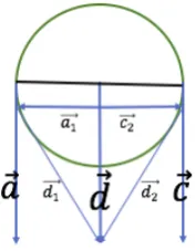
Figure 3.Vectors~a,~c,d~as well asd~1and~d2which are pointing in the direction of increasing gravitational force.(Appendix).
parameter is introduced whereby in the large limit case a method of solution is sought for in the 67
boundary layer of the tube. By seeking an additive solution using the continuity equation and the 68
simplified vector equation obtained by a similar procedure and using the product rule of differentiable 69
calculus, and using Geometric Algebra as a starting point, it follows through analysis that the integral 70
of total divergence of a specific vector field over time can be expressed as the integral with respect 71
to time of the line integral of the dot product of inertial and azimuthal velocity. The line integral is 72
evaluated on a contour that is annular and traces the boundary layer as time increases in the flow. It 73
has been shown that a reduction of the 3D compressible unsteady Navier-Stokes equations to a single 74
partial differential equation is possible and integral calculus methods are applied for the case of a body 75
force directed to the centre of the tube to obtain an integral form of the Hunter-Saxton equation. Also 76
an extension for a more general body force has been shown where in addition there is a rotational force 77
applied. 78
6. Appendix 79
Referring to Fig.3, let,
~
d=k~a (53)
~
d=m~c (54)
It follows that,
~
d+~d
2 =~d=k~a+m~c (55)
If~aand~care in the same direction thenkm>0 andk,mare either both positive or both negative. Also according to Fig.3 it follows that,
~
d 2
=k~c2k2+
~
d2 2
(56)
d~
2
=k~a1k2+ d~1
2
(57)
If the circle shrinks to an arbitrary small circle in diameter then
d~
2
≈
d~2 2
d~
2
≈
d~1 2
(59)
Summing up all thedicomponents and lettingb2ieθrepresent the tangential velocity for each point on
the circumference of diskR, it follows forNdistinct points that, N
∑
i=1di= N
∑
i=1b2i (60)
Thus in the limit as the circle diameter gets small, introduce a functiongdefined as,
g =
∂b2
∂θ (61)
where~b=b2~eθand ∂
~b
∂θ is the vector pointing towards the center of the disk inR.
80
81
Acknowledgment 82
83
1. G.K. Batchelor,An introduction to fluid dynamics, Cambridge University Press, (1967). 84
2. R. Cai,Some Explicit analytical solutions of unsteady compressible flow, transactions of the ASME, Journal of 85
fluids engineering, Vol. 120, (1998), 760-764 86
3. A.J. Chorin,The numerical solution of the Navier-Stokes equations for an incompressible fluid, Bull. Amer. Math 87
Soc. Volume 73 No.6, (1967), 928-931 88
4. C. Doran, A. Lasenby,Geometric Algebra for Physicists, Cambridge University Press, (2003). 89
5. D.G. Ebin,Motion of a slightly compressible fluid, Proc. Nat. Acad. Sci USA, Vol 72,No.2, (1975), 539-542. 90
6. M. Feistauer, J. Felcman and I. Straskraba, Mathematical and computational methods for compressible flow, 91
Clarendon Press-Oxford Science Publications, (2003). 92
7. T. Moschandreou,A New Analytical Procedure to Solve Two Phase Flow in Tubes, Math. Comput. Appl. 2018, 23, 93
26. doi: 10.3390/mca23020026 94
8. L. M. Pereira, J. S. Perez Guerrero and R. M. Cotta,Integral transformation of the Navier-Stokes equations in
95
cylindrical geometry, Computational Mechanics, Volume 21, Issue 1, February (1998), 60-70. 96
9. C. Taylor, P.Hood,A numerical solution of the Navier-Stokes equations using the finite element technique, Computers 97
and Fluids, Volume 1 Issue 1, (1973), 73-100 98
10. P. Vadasz,Rendering the Navier-Stokes equations for a compressible fluid into the Schrödinger Equation for quantum
99