Local movement: agent-based models of pedestrian flows

Paper 4

LOCAL

MOVEMENT

AGENT-BASED

MODELS OF

PEDESTRIAN

FLOW

Michael Batty

Bin Jiang

Mark

Thurstain-Goodwin

CENTRE FOR ADV

ANCED

SP

A

TIAL ANAL

YSIS

W

Centre for Advanced Spatial Analysis University College London

1-19 Torrington Place Gower Street

London WC1E 6BT

Tel: +44 (0) 171 391 1782 Fax: +44 (0) 171 813 2843 Email: casa@ucl.ac.uk http://www.casa.ucl.ac.uk

http://www.casa.ucl.ac.uk/local_movement.doc

Date: June 1998

ISSN: 1467-1298

© Copyright CASA, UCL.

ABSTRACT

Modelling movement within the built environment has hitherto been focused on rather coarse spatial scales where the emphasis has been upon simulating flows of traffic between origins and destinations. Models of pedestrian movement have been sporadic, based largely on finding statistical relationships between volumes and the accessibility of streets, with no sustained efforts at improving such theories. The development of object-orientated computing and agent-based models which have followed in this wake, promise to change this picture radically. It is now possible to develop models simulating the geometric motion of individual agents in small-scale environments using theories of traffic flow to underpin their logic. In this paper, we outline such a model which we adapt to simulate flows of pedestrians between fixed points of entry - gateways - into complex environments such as city centres, and points of attraction based on the location of retail and leisure facilities which represent the focus of such movements.

Local Movement in the Urban System

Below a certain scale particularly where spatial representation is more appropriate in

terms of the built form rather than territorial subdivision, aggregative approaches to

explaining and predicting urban phenomena begin to lose their meaning. For example,

in town centres, in shopping malls and housing estates, location and movement is best

described in terms of the individuals who use such spaces rather than in terms of their

aggregation by social or any other attribute. Predicting local movements, patterns of

crime, deprivation, and the individual usage of urban facilities must thus be simulated

by treating the populations involved as distinct ‘objects’ or ‘agents’. Such approaches

although still novel are not inconsistent with the more aggregative approaches which

have dominated urban simulation hitherto, but at scales where buildings, public

spaces, and streets must be represented as distinct objects, the associated behaviour

patterns of individual users must be directly simulated if impacts of changes to the

geometry of the local environment are to be understood.

To date, there have been few long term efforts to simulate the patterns of pedestrian

flow within small scale environments. Despite the fact that walking in western cities

constitutes up to 30 percent of all journeys made (GSS, 1997), and in city centres such

as the West End of London up to 40 percent (Whiteley, 1997), this mode of travel has

been almost entirely neglected in mainstream transportation modelling which still

emphasises the automobile. Early attempts at modelling pedestrian flows followed

three rather different approaches. Descriptions of how pedestrians move and

congregate have provided statistical data for the distributions of queues, and these

have been used to predict volumes on street segments from linear relationships

estimated by regression (Older, 1968; Stilitz, 1969; Sandahl and Percivall, 1972).

More formal approaches based on loose analogies with fluids, gas kinetics, and other

physical flow systems have been proposed and tested (Henderson, 1971, 1974;

Helbing 1995) but by far the most usual approach has been based on adaptations of

spatial interaction models, often in their discrete choice rather than gravitational form.

Attempts to simulate pedestrian flows (Borgers and Timmermans, 1986a, 1986b)

developed, but the predictions from such models must then be scaled back to more

aggregate units if they are to be generalised spatially. Models of movement patterns in

the urban system based on microsimulation appear promising but notwithstanding the

effort that has gone into such simulation in recent years (Clarke, 1996), there have

been very few applications at a fine spatial scale. Such approaches concentrate on

simulating generic patterns or profiles within a population based on ‘typical’ or

‘prototypical’ individuals but ways of mapping these profiles onto detailed spatial

representations are poorly developed.

There has been more activity of late in associating movement patterns and the location

of pedestrian volumes with measures of spatial accessibility, proximity, or

connectedness. Since the 1940s, measures of accessibility based on evaluating the

potential of any location with respect to how near and how attractive it might be to all

other locations have been used to provide indices which show the actual or potential

density of use at any location within the city or regional system. For example,

Hansen’s (1959) residential land use model was based on forecasting growth or

change at any location in proportion to the value of its accessibility, based on a variant

of Stewart and Warntz’s (1958) measure of population potential. In terms of

networks, the density of traffic flowing across any node has been correlated with

degrees of nodal connectivity within such networks (see Haggett and Chorley, 1969)

while a more recent theory of natural movement due to Hillier et al. (1993) has sought

to correlate movement patterns at the local scale with the relative accessibility of

streets to one another. This theory, referred to as space syntax, is a first order

generalisation of accessibility or connectivity of streets where streets are treated as

nodes and network measures computed if streets relate to one another in various

physical ways such as through their intersection. However, these accessibility

measures although providing indices associated with forecasting trip volumes, are not

based on models which simulate processes of movement and thus do not provide

methods for predicting the impact of locational changes on patterns of pedestrian

flow. In short although these indices can show changes in flow due to changes in the

geometry and location of entire streets, they are unable to account for comprehensive

movement patterns which link facilities at different locations to one another. Although

space syntax deals with movement economies, it has not yet been possible to link

1997).

The need for a much richer theory of local movement accounting for individual

behaviours which determine pedestrian flow suggests that all aspects of the

environment within which such behaviour takes place as well as the individuals

generating such behaviour must be represented explicitly, as distinct objects. Recently

object-oriented approaches to simulation have become popular due to developments

in programming technology as well as due to the increasing perception that local

behaviour is fundamental in explaining global pattern. To develop models of such

local behaviour, individuals must be represented explicitly and from this comes the

idea of ‘agent-based’ modelling (Axelrod, 1997a). This is entirely consistent with

recent developments in complexity theory where the complexity of the system

emerges in global and structural terms from actions, each of which are simple in

themselves, of relatively autonomous agents, acting with their own self-interest in

mind, without appeal to any grand design or response to any overall global rationality

or utility. Models for simulating artificial life are the best exemplars (Langton, 1995;

Adami, 1998). Of course many systems cannot be characterised in this way but local

movement patterns and behaviours in small-scale built environments appear to fit the

approach rather well.

Small-scale environments capture the global properties of the urban system in such a

way that local responses are usually consistent with macro properties. For example,

local geometries such as the juxtaposition and type of buildings, the scale and

direction of streets, and the location of transport facilities all imply a global order to

the city. Thus when individuals respond to what is in their immediate neighborhood,

this will reflect a more global order. The relative attraction of facilities at different

locations is usually mirrored locally and local responses are thus consistent with

behaviours which reinforce the global order. For example, if an individual is searching

for an attractive retail location and is in a relatively unattractive location, then the

local situation is likely to contain clues as to how to move towards a more attractive

location. However, local movements are also heavily influenced by much more

idiosyncratic factors such as physical obstacles around which to navigate, localised

congestion, and serendipitous decision-making with respect to what is immediately

ranging from movements which are well-defined and completely purposive to those

which are more random and exploratory, based on walkers who know the

environment completely to those who do not know the local geometry and attractions

of the environment at all. An agent-based approach is the only way in which we might

account for such diversity and design models which can be tuned to quite different

walker situations.

A number of agent-based models are being developed which have direct relevance to

smallscale urban environments. The TRANSIMS model under construction at Los

Alamos (which is associated with the elaborate microsimulation system called

SWARM) has been developed to model individual trip movements at the level of the

automobile (see http://www.lanl.gov/). The model system is noteworthy because it can

be simplified in various ways to show its consistency with various major themes in

complexity theory such as local movement based on cellular automata ideas as well as

self-organised criticality (Nagel and Paczuski, 1995). It is perhaps the most developed

such system to date and lies one step beyond the ideas we will develop here. As such

it represents a potential next stage in our own research. A much more focused set of

approaches is being developed by Helbing and his co-workers at Stuttgart who have

developed several variants of pedestrian model, particularly based on analogies

between social and physical forces (Helbing, 1991; Helbing and Molnar, 1995). In

these models, the patterns of walking are reinforced by the very activity of walking,

such that the system and its movement patterns self-organise according to certain

interactive behaviour (Helbing and Molnar, 1997). However although TRANSIMS and

these active walker models incorporate many relevant features of local movement,

their purpose is less geared to predicting the importance of locations to which

pedestrians move than the approach that we will develop here.

Other models of local movement in which location is prominent are those in which

actors or agents respond to others in their vicinity. For example, the range of models

developed onwards from the work of Schelling (1978) in which actors move or

migrate to be closer to those to whom they perceive some affinity, thus creating

polarised clusters or ghettos, might be adapted to deal with local movements. Their

focus however is on longer term spatial migration rather than the more routine and

polarisation based on cultural convergence and Epstein and Axtel’s (1996)

‘Sugarscape’ model of an artificial society are more recent variants on this theme that

provide exemplars of why agent-based approaches are essential. Finally, the models

which emanate from the simple manipulation of local geometry as embodied in the

multiple Logo approach developed by Resnick (1994) amongst others, are well

adapted to dealing with local movement as illustrated in a variety of examples such as

insect movement, trail formation, and percolation through sparse and dense media.

These are all rooted in the logic of cellular automata to which we will return.

There are more pragmatic reasons for developing agent-based models of small-scale

urban environments. First there is a strong commercial imperative for predictive

models which are able to simulate how attractive different locations are to consumers.

The location of points at which such consumers are ‘discharged’ into spatial markets,

the characteristics of streets which enable such consumers to reach the market sites in

question, and the relative attraction of other adjacent sites all directly affect profit

margins through patronage. The same issues pertain to sites in the leisure industries

which rely upon visitors. More focussed social concerns such as the spatial incidence

of crime, and the need for secure environments are intrinsically bound up with the

location and type of facilities and the extent to which these are patronised. In one

sense, the problem emphasised here is little different from the more general problem

of urban location at larger scales except for the interaction between local geometry

and purposive and exploratory behaviours which seek to optimise locational

attraction. The fact that such modelling is now possible also relates to the availability

of new data sets, many of them collected by the various commercial interests which

have greatest need for good predictions involving their retail trade. Good digital data

on built form is now available at 1-2 meter resolution while pedestrian flows are being

increasingly monitored automatically and remotely using closed circuit TV.

Questionnaire surveys of origin and destination movement patterns and

person-following techniques for precise walking inventories are increasingly available. Data

from electronic point-of-sale (EPOS) is being associated with spatial and locational

data at a variety of scales, from movement within the store at one extreme to

movement within the metropolis at the other.

require different variants of this approach and at the outset, we should be clear as to

the issues that we consider important and those that we will ignore. Our model will

apply to relatively closed geometric systems such as malls and town centres, galleries

and theme parks within which visitors or walkers engage in purposive activities such

as shopping or leisure for fixed periods of time. We will make the assumption that all

the individuals who move within such systems enter and leave the system at the same

points (although we can easily relax this) which we will call ‘gateways’. In each case,

an individual’s trip can thus be divided into active and passive stages where we

assume that an individual is active for most of the trip but once a decision is made to

return to the gateway, the trip becomes passive in that the goal changes from visiting

the most attractive locations to that of returning to the gateway. In this sense, the

variants of the model that we illustrate here will not apply to movements in residential

neighborhoods or in work trip contexts. Furthermore, all our experiments will be of an

exploratory nature. These kinds of pedestrian model are in their infancy and it is likely

that very different versions of them will emerge once the research momentum builds

up. We consider that all such models so far are ‘proofs of concept’ rather than fully

operational predictive structures. However this does not imply that we cannot gain

insights from such applications.

In the next section, we will outline the key issues that characterise the kinds of local

movement we will simulate, illustrating the rudiments of the model and the way these

can be articulated. We then develop the mathematics of our generic model, showing

how a typical walker moves through the geometric system and interacts with other

walkers within the same space. We implement the model as a cellular automata, using

highly visual software which enables us to examine movements and patterns as they

take place in the geometric space which we visualise through a variety of map layers

and agent movements. We then develop three related applications or experiments, Our

first experiment involves the simplest model - an idealised retail mall based on a

symmetric geometry with a simple unimodal retail attraction surface. We show how

the pedestrian movement can be varied as various parameters controlling the

interaction of the local geometry with the surface attraction can be manipulated, thus

illustrating how we can ‘calibrate' the model. Our second example, involves the same

model applied to a real town centre, that of Wolverhampton which is a medium sized

attempt to calibrate this model in the conventional way by searching over the

parameter space for parameter values which generate patterns of realistic-looking

movement. Our last experiment involves introducing considerably more complexity

into the model through very complex local geometry that characterises the space as

well as the more complex locational attraction posed by a structure of closed rooms

linked by galleries and corridors. We show how we can model pedestrian visitor

movements in London’s Tate Gallery and then outline how the model can be

calibrated to real data which provides realistic simulations of movement, by letting the

agents ‘learn’ the best parameter values as they move through the space. Finally we

draw these various threads together, speculating on next steps in the research

programme and arguing the need for taking this research to a more sophisticated level

of simulation.

Representing Pedestrian Flows

The generic framework we develop will be flexible enough to take account of several

different problem characterisations, all of which involve relatively self-contained local

movement. However, this framework is based on the requirement that pedestrian

movements are important to predicting how many individuals are attracted to different

sites within the local system of interest. The flow volumes on the various routes that

relate these sites are of interest but the detail of the flow is not relevant. In essence,

the model allocates walkers from fixed origins to various destinations and in doing so

enables their assignment to the various streets, sidewalks, squares and precincts which

link origins and destinations together. The elements of the model loosely reflect ideas

of attraction and deterrence in more aggregative traffic models that build on traditions

in spatial interaction modelling (Willumsen and Ortuzar, 1990). Other aspects of

pedestrian flow are of lesser interest; for example, the streaming of pedestrians, their

movement in groups, their behaviours at street intersections, gates and doors, and their

velocity are of little relevance as the focus here is upon the location of origins and

destination, the geometry of their linking, and the flows which bind various locations

together. Lastly as we have already implied, trips in this kind of system begin and end

at the same origin and exist over a fixed interval of time such as a shopping trip

behaviour. The interest is upon how many visits are made in total to various

destinations, notwithstanding the fact that those controlling or managing such

destinations might be interested in more detailed temporal movements.

In any model, it is possible to relax assumptions but we will begin by specifying the

model in the strictest form possible. All origins are referred to as gateways. These are nodes in the system such as car parks or bus stations from which walkers are

‘discharged’ and from which they begin their walk through the system. We will

assume that at each gateway, individuals change their transport mode - in car parks

from car to walk, in bus or rail stations and at bus or rail stops from bus or rail to

walk. The same kinds of transition can be assumed for linear gateways such as

on-street parking lines; for those who walk directly into the system from outside, we

assume a line of gateways surrounding the system from which these walkers assume

their pedestrian mode. Related to this assumption is the fact that all pedestrians return

to the gateways from which they enter the system. This is not so severe an assumption

as it might appear and it has only been introduced to simplify the simulation; if

necessary it can be relaxed.

While gateways are always discrete points, we represent destinations somewhat differently, as continuous attraction surfaces which cover the entire extent of the local geometry. This is primarily due to the fact that such surfaces can be easily

computed from very detailed point location data using various spatial averaging

techniques. These enable each location in the system to be considered relative to any

other, and thus to be independent of the local geometry of buildings and streets. In

short, this is a way of aggregating and smoothing out the effects of individual

buildings and stores and also of adding together various data to produce composite

indices of attraction. For example, such attractions might be built up from data on

retail turnover, floorspace, rents and so on, most of which are not available for

individual shops but are available for very fine scale geometries such as postal

delivery codes. This implies that a large store in the centre of town is likely to have a

level of attraction per unit of its space rather similar to an adjacent store which is

much smaller, selling different goods, and attractive to different customers. This

example, in the Tate Gallery example, the attraction surface is based on rooms which

are disjoint from one another but with equal levels of attraction within each room.

Finally, it is quite possible to have more than one surface of attraction, each picking

up different features of attraction at various locations, and being either combined or

used sequentially through the walking process.

The third element of representation involves the local geometry of buildings and

streets - the built form. The kind of resolutions that we are concerned with here range

down to 1-2 meters. Fairly precise movements can be modelled at this level but to

model very detailed interaction of pedestrians with one another in the manner which

the Stuttgart group have employed (Helbing and Molnar, 1995), it would be necessary

to represent the system down to 0.1 meter resolution so that crowding could be

thoroughly examined. Our limit is consistent therefore with our interest in aggregate

flows and flows attracted to different locations. Our characterisation does not pick up

the kind of detail where one walker might relate to another except in terms of total

counts of crowding. For example, we do not simulate how two walkers might collide,

nor do we simulate how they might behave at intersections or at doorways. However,

our model should be able to detect crowding which occurs as pathways and streets

narrow. It should also reflect the intrinsic attraction of the sidewalks along buildings

relating to the fact that streets never go directly to the points of highest locational

attraction (which are within buildings) although walkers attempt to do so. Lastly, we

will not simulate the behaviour of pedestrians who might act in groups other than

through the usual mechanism of increasing attraction as more pedestrians visit a place

or reducing attraction as congestion thresholds are passed.

We can now outline the key principles for movement which we will build into the

model and which we believe are borne out through current observation and our causal

knowledge of how walkers behave in small-scale urban environments. Our walkers

move one step in each time period (if they are able) and this is in a given direction

which in turn is measured through an angular heading or through xy coordinates. We

define five components which determine direction in each time period of the

simulation:

attraction. At any location and at a given time, a walker who is still engaged in

active movement in the system (that is, not returning to their origin or gateway),

sets a heading in the direction of the gradient of the attraction at that point. In the

case where there is a unimodal surface of attraction with the highest point at the

centre of the town say or at the prime retail pitch, the walker will continually

readjust this heading in an effort to climb to the top of the surface: the

hill-climbing analogy is relevant. There are many factors that might obstruct this

process; where there might be multiple local optima or several surfaces of

attraction evaluated in sequence, say. But the most likely changes in direction

which distort this process are due to the interaction of the surface with the local

geometry as we will indicate below.

2. The default direction in the model is for any walker to move in the direction that

they are already travelling, that is forward. In each situation where the walker is

moving forward, this heading is perturbed by a random change in direction whose

probability of occurrence declines proportionately and nonlinearly with the size of

the deviation from the forward direction.

3. Obstacles to forward movement occur through the local geometry of streets and

buildings. At each stage of the walk, a running count of progress in terms of

distance travelled is kept. If a walker hits an obstacle such as the edge of a street,

the walker continues to advance with their heading perturbed randomly. If after a

number of tries, no progress has been made, the walker reverses direction and

several new directions are tried until one which initiates progress is found.

4. At a given time period, the level of congestion at each location in the system is

evaluated. If there are more walkers at or around a point than a predetermined

threshold, then walkers are perturbed in terms of their subsequent directional

movement until congestion falls below the threshold.

5. In different areas of the spatial system - rooms for example in a gallery, or squares

and street segments within a town centre, change in the number of walkers and

their totals are measured in each time period. These changes and totals can be

the point when congestion sets in and attraction declines. In this way, the number

of walkers in any area can also be controlled.

Walkers are thus connected to one another through locational attraction and through

congestion. In this way, various positive feedbacks are reinforced and the system can

be self-organising in a similar manner to that used in the models developed by the

Stuttgart group (Helbing and Molnar, 1997).

Movement is calculated in each time period t in the direction r for each walker k,

where k = 1, 2, ..., K, there being K walkers in the system. K will vary with time t but

to introduce the model, we do not need to detail the way K changes yet. Each location

in the system is given by coordinates xy (which pertain to pixels in the computable

model developed below), and thus the direction of each walker is defined as

r x y t_{k( , , ) . In the model, we will compute direction from the heading θ at xy where}

0< <θ 2π θ_{, being measured in radians. However we will first state the model in} general terms in this section before we develop its computable form in the next. In

general, the direction for any walker k at time t + 1 is defined from

r x y t_{k i}f_i i ( , , ) =

∑

τ

(1)

where fi _{is a function of one of the five components affecting the heading, and}

τ

If for example, this switch applies to every time period and every function, then

τ

write equation (1) explicitly for the five components as

r x y t_k( , , ) =

τ

τ

τ

τ

τ

(2)

surface at xy, fd is the function involving movement in the forward direction which is

the default, fb _{is the function that controls the perturbations needed to navigate a}

physical barrier, fc _{is the congestion function that involves perturbing the direction of}

any walkers who are exceeding the threshold, and fa _{is the function that enables the} attraction surface to be updated with respect to the number of walkers in that area of

the system in question.

Each of these functions should be further defined so that the elements involved in

each can be specified prior to the full model being stated. The direction r x y tk( , , ) is defined as a sum of each of five components which in turn are evaluations of the

heading required to make independent progress in each of the five directions. Which

are relevant depends of course on the temporal switches {

τ

vector. The first component fg _{is a function of the attraction surface}

ϑ

[

]

f_g = f_g ∇

ϑ

, (3)

while the second function fd_{, the default forward direction with random perturbation}

ε

[

]

f_d = f_d r x y t_k( , , ),

ε

. (4)

The third component involves the perturbations required to avoid locations within the

[

]

f_b = f r x y t_{b k}( , , ),{ ( , )}B x y

. (5)

The fourth and fifth components are those which lead to direct positive feedbacks

between walkers. Congestion is computed as the sum of walkers k in the congestion

neighborhood of point xy, called Zxy_{, with appropriate perturbations}

ω

[

]

f_c = f_c {

∑

ω

χ

, (6)

while attraction ϑxyt _{is altered according to the number of walkers in the attraction}

area Ωxy _{within which the point xy exists}

[

]

f_a = f_a {

∑

ϑ

. (7)

The precise functional forms for these five components will be specified below. The

simultaneity which is implied in equations (1) to (7) is resolved in the computable

model once these forms are made discrete and the sequencing implied through {τi} in equations (1) and (2) is specified.

A Computable Form for the Generic Model

We will first examine the five components of movement and then show how these are

assembled into the integrated model before dealing with detailed algorithms and

programming in the next section. All movement in the model is driven from setting a

new heading θ in each time period t for each walker k henceforth referred to as walker _wk at location xy. As we have indicated, we assume that each walker k makes a

unit step forward or remains stationary in each time period and this implies that

chosen so that r x y tk( , , )= ∀1, kxyt. In the following outline, we will suppress the indices k, x, y, and t wherever it is obvious from the context. Changes in direction are computed from

∆x=r x y t_k( , , ) cosθ and ∆y=r x y t_k( , , ) sinθ

where using the assumption of unit length in walking, the new coordinates become

x_t+1 =x_t +∆x=x_t +cosθ_{, and (8)} y_t+1 =y_t +∆y= y_t +sinθ _{. (9)} Equations (8) and (9) apply to the evaluation of any motion, whether or not the walker

is in the active or passive (returning) phase of their trip and whether or not this motion

actually takes place.

The first and most basic component which affects each walker’s heading is the

function involving the gradient of the attraction surface fg = fg

[

ϑ

]

∇

ϑ

∂ϑ

∂

∂ϑ

∂

xyt

xyt xyt

x y

(10)

from which changes in direction can be computed in proportion to

∆ ′ =x

x dx xyt

∂ϑ

∂ _and

∆ ′ =y y dy xyt ∂ϑ ∂ _. (12)

A notional single step distance of dx = 1 and dy = 1 implies that progress is directly proportional to the partial derivatives of the surface in their respective directions. In

fact the angular variation can be directly computed from

θ

∂ϑ

∂

∂ϑ

∂

tan 1 xyt / xyt

x y

(13)

where θ is used to update the heading and to define the increments ∆x and ∆x in equations (8) and (9).

The second component is based on a function fd

[

ε

]

on the assumption that walkers continue in the direction that they are going but with

some probability that they will adjust their heading marginally. The adjustment, an

increment to the heading ∆θ is defined from

∆θ = ±{ /π random(100)} (14)

where it is clear that the absolute value of ∆θ varies inversely with the random occurrence of any number in the uniform interval [1:100]. 90 percent of the time, this

value will be less than 18 degrees or 0.314 radians. This perturbation to direction is

applied to all headings, including those which are computed from the other four

components.

whether or not the forward motion computed from any function hits a geometric

barrier or obstacle in the set {B x y( , ) }. If the new coordinate pair

[

]

then no movement takes place because the location is not part

of the system where walking is allowed. In such cases, a progress variable λkt_, measured in terms of distance travelled, is set as 0, and the walk continues; each

subsequent time period, this variable is accumulated and tested to see how much

progress has been made. If progress is less than a certain threshold Λ, then it is assumed that the obstacle cannot be circumnavigated without the walker reassessing

its position and heading. Formally

if λ_kt <Λ,then x_t′ =₊₁ x_t −∆x and y_t′ =₊₁ y_t −∆y (15)

and the walker attempts to reverse. If

[

]

reassessed as

∆θ =random{2π} (16)

and the algorithm implied by equations (15) and (16) is repeated a preset number of

times m. m is 6 in the experiments reported here but like the progress threshold Λ, it is a parameter of the system and can be calibrated if required.

The last two functions - the fourth and fifth components - involve introducing

interactions between walkers. The component

[

]

f_c {

∑

ω

χ

counts the level of congestion in the vicinity

Z_xy

N_xyt w_k k Zxy

=

∈

∑

.

(17)

Then if Nxyt <χ, _{the headings of the relevant walkers in} Zxy _{are perturbed by a} directional component [ωk( , , )]x y t _{although in practice this is achieved by setting the}

heading to ∆θ =random{2π} as in equation (16) above. There is no guarantee that this will reduce the level of congestion per se although combined with other

processes, it appears to work effectively. So far, we have set Zxy _{as single point} locations because the scale of resolution for the examples we have developed is such

that this is appropriate. However, this set can be modified in terms of area covered if

required.

Finally, the function fa

[

∑

ϑ

]

number of walkers in the area Ωxy _{where this might be a square, a segment of street, a} shop or a room within the system in question. We first count the number of walkers

M_xyt

in the set as

M_xyt w_k k xy

=

∈

∑

Ω

(18)

arguing that the attraction ϑxyt _{is proportional to the number of walkers visiting the} place. Of course, we preset the locational attraction surface in most cases but we are

able to modify this preset attraction to take account of economies and diseconomies of

scale not built into the simulation through prior data. For example, we can set the

ϑ

ϑ

β

β

where equation (18) is clearly parabolic, implying that for small values of Mxyt,ϑxyt+1

is an increasing function of the number of walkers in Ωxy_{, while for larger values, this} function is decreasing. The precise form will depend upon the parameters β1 _and β2

while the baseline value of the function is set to the prior value of locational attraction

ϑxy _{which is input data. So far in our simulations, we have not conducted exhaustive}

tests of this device although we consider the function important in pushing the model

towards greater realism. It will be of particular use in later applications where we

divide walkers into those who already know the space in which they are moving and

those who do not. The latter group will move in response to those already in the

system, being influenced by prior movement which is captured through changes to the

attraction surface that they respond to and which will be computed in the manner of

equation (19).

All the components of movement have now been assembled but as equation (2)

implies, these five functions can act differentially in time. As this is important to the

logic of the process, it is necessary to demonstrate how these functions are nested and

sequenced within the model. The order in which these five components are evaluated

as well as the points at which they are switched on and off combine to produce quite

complex modulations. The temporal switches {τi_{} differ in form. The congestion}

switch τc is either on or off; if off, the function fc is never evaluated while if on, it is evaluated at each time period. When this switch is on, and if the congestion level is

exceeded at any location, then walkers are moved within a time period, that is they are

moved immediately, and thus this factor does not affect any of the other functions. It

can be operated anywhere within a time period, and in the current version of the

model, it is evaluated first.

function fb are switched regularly but occasionally in the current implementation,

usually on different sequences but the switches τg_, τ_{a, and} τ_{ib can be set to any time} series, the default being their operation at every time. The current model evaluates

gradient before attraction before barriers but in the case of the barriers function, a

barrier must have been encountered and less progress made than the given threshold,

for the function to be activated. However, an order of precedence is established when

the time switches coincide; the barrier takes precedence over the attraction level

which in turn takes precedence over the use of the gradient to fix the new heading of

the walker. At this point, it is worth noting that only the congestion and barrier

functions apply to walkers who are in the passive state, returning to their point of

entry or their gateway. When these functions are not being activated - that is, when

there is no congestion or no infringement of a barrier - then the heading of a returning

walker is fixed to ensure that progress is made back to the gateway. This heading is

fixed before the final function - perturbation in the directional heading - is invoked.

This function fd _{controlled by the switch} τd _{is always switched on in this model, that} is, it operates in every time period. It is evaluated last and this means that the

dominant heading determined by any of the functions already evaluated or the heading

on the previous time period if none of the functions just discussed have been activated

in that time period, is perturbed in the usual manner. This incorporates local

fluctuations in movement which always occur in reality.

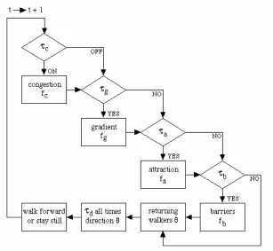
The logic of these operations is illustrated in the flow chart in Figure 1 where it is

immediately clear that what operates in each time period depends upon the way in

which the switches are configured and the order in which the five components are

evaluated. In the default case where all functions operate in each time period, then the

congestion function always applies and is self-contained while the barrier function if

invoked will always take precedence over the attraction function which in turn

dominates the gradient function. Note that when the attraction function is evaluated,

then this involves the computation of a new gradient. The directional heading function

of course applies in every time period. The critical sequencing then depends on the

frequency at which the gradient, attraction and barrier functions are evaluated. The

For example, if the gradient function is evaluated in every 5th time period, the

attraction in every 7th and the barrier in every 4th, then only in the 140th period will

the barrier take precedence if operative. However, various combinations of these

frequencies would mean that the following sequence would apply: when t = 4, fb_{; t =}

5, fg_{; t = 7,} f_{a; t = 8,} f_{b; t = 10,} fg_{; t = 14,} f_{a; t = 15,} f_{b; t = 16,} f_{b; t = 20,} f_{b; t}

= 21, fa_{; t = 24,} fb_{; t = 25,} fg_{; t = 28,} fb_{; t = 30,} fg_{; t = 32,} fb_{; t = 35,} fg_{; ...;}

t = 140, fb_{; and so on ...}

As well as the structural logic that we have developed which determines the

precedence of certain operations, the model has several parameters which need to be

specified and calibrated. As it stands, it represents a subtle combination of local and

global factors and functions, based on the way local geometry combines with global

attraction. Some might argue that such models should be based on local factors

entirely and that local geometry should determine the way walkers respond and use

various attractions. This may be the case for situations where visitors have no

knowledge of the local situation but in systems where some idea of the global

properties of the environment are known from previous contact which is often, in fact

usually the case in town centres and shopping malls, then some global functions are

essential. Moreover these models are ones which simulate routine movements; they

are not meant to enable trails to be formed or paths and streets in cities to be

developed. They are much more akin to traffic distribution and assignment models

than to evolutionary models. Although we have added a fifth component dealing with

the modification of attraction based on movement volume, we consider this to be a

factor which enables congestion to be handled, rather than mirroring any real

Figure 1: Components forming the Walking Algorithm

Implementing the Model as a Cellular Automata

The way pedestrians use town centres and malls has been conceived here as a

bottom-up process, in which walking is a subtle interplay between the effects of local

geometry, attractions which are ‘discovered’ as walkers move, and more global

attractions which provide an overall rationale for such trip making in the first place.

As we implied earlier, there are several ways in which such simulation might be

implemented based on the rationale of spatial interaction modelling or

microsimulation of event and agent profiles, although the emphasis we have given

does provide quite strict limits on the extent to which global factors can be treated in

that most functions in such frameworks deal with entirely local neighborhoods, thus

making it hard to examine any phenomena of interest at a distance from any given

location. However with judicious use of neighborhood data within which global

features are contained, such simulations can be very effective.

We make an initial distinction between agents in this case pedestrians or walkers

-and the environment in which motion takes place. The environment is always

conceived as a 2-dimensional space based on a homogeneous grid of pixels which

represent xy locations, upon which various characteristics or attributes of the environment can be stored as spatial layers. Agents also have characteristics and

attributes, and motion depends upon the interaction between agents and their

environment as well as interactions between agents, both types of interaction being

effected through comparisons of attributes. The local geometry and the global

attraction of locations are represented as part of the environment while agents move

by making comparisons between these characteristics of the environment and their

own motivations for motion which are represented by their personal characteristics.

For example, a walker, who is actively shopping, will respond to the environment in

terms of attractions and geometry in a different way from a walker who is returning

from such a trip to their point of entry or gateway into the system.

Agents are virtually ‘blind’ in such a system in that the CA principle restricts their

viewshed to their immediate neighbourhood. This is useful for evaluating immediate

obstacles but is quite limited for evaluating progress which depends on lines of sight

and memory of destinations. Because streets and even squares and precincts tend to be

directional for the most part, once a walker is set on a heading which makes progress,

then this is reinforced by the model with walkers following lines of sight from the

interplay of the local street geometry and the behavioural need to maintain direction.

More global factors must therefore be encoded locally through the attributes of layers.

Where there is a global optima to location - represented as a unimodal attraction

surface for example, then the local gradient is sufficient for walkers to make progress.

More complex surfaces, however, must be disaggregated into constituent and simpler

parts which are handled by walkers separately. A spatial interaction model, for

complex attraction directly whereas in CA modelling, only the immediately adjacent

locational attractions can be examined. If these are to be used to influence direction,

then these must embody some local element which reflects the global attraction; this

is the case where the surface is particularly simple and the local gradient is the key to

where the walker is on the overall surface (Batty, 1998). It is possible in CA to

decompose the surface into different trends, each implying some significant

destination but the number of such decompositions is limited.

In short, only for certain problems is the CA approach relevant. Problems where there

are many local optima or where trip making is dominated by very specific destinations

are likely to be unsuitable. Here the Tate Gallery exemplar is instructive for visitors to

the gallery are likely to be newcomers, most being first time visitors to the particular

exhibition and thus movement is dominated by much exploratory walking. As there is

only one gateway or entrance, then there needs to be a global function relating to

drawing walkers into the gallery and this is set up as an orientation surface. The local

attraction of different rooms provides another surface and the way the model works is

by interweaving these two surfaces in such a way that combined with local geometry,

realistic walking patterns are simulated. Nevertheless, such ideas are fairly

experimental as yet and all we can say so far is that this approach appears promising.

CA is a very effective approach for processing local information rapidly and

efficiently (Toffoli and Margolus, 1987). The version we use here makes a distinction

between agents and environment in the manner we noted above and is based on

Resnick’s (1994) version of Logo (called StarLogo) where multiple agents (called turtles) interact with a spatial environment whose layers (called patches) contain the

geometric and other characteristics of the spatial system. This system can handle up to

16K agents, spatial environments up to 200 x 200 cells in size (arranged in grid/pixel

fashion) whose attributes can be encoded in up to 64 layers. The software provides a

means for rapid prototyping of these kinds of model. The visualisation capabilities of

the system are good, with a user-friendly interface for modelling operations, fast

animation of dynamic change, in this case motion, and the ability to visualise layers at

will. The agents can be individually interrogated as can the cells which comprise the

environment and this enables the numerical state of any agent or cell to be examined

yet, we have not invoked these functions. A feature of the software is that parallel

processing is simulated in that all updating of agent behaviour is made

simultaneously. The program can be stopped and started at any time and parameters

can be changed on-the-fly. Although we have structured the walk routine quite

formally as we illustrated in Figure 1, it would be possible to set up each of the five

components of motion as independent modules, which would run separately, the

parallel processing compiler taking care of the order in which these operations were

effected. Although this is attractive and we will consider it in later applications, the

current logic follows the sequential mode of operations shown in Figure 1.

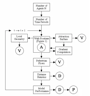
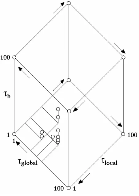
The structure of the program is shown in Figure 2. It is built around the walk routines

with local geometry and global attraction providing the key inputs. These layers

provide data which control the walk routines, but they also provide the backcloth on

which various inputs, outputs and the animation itself can be visualised. The open

circles labelled A, V, D, and P represent program modules which are called to animate the walks (A), visualise the geometry and surfaces (V), display numeric data

(D), and plot such data (P). As in many visual programs, the data concerning the built

form, the gateways - entry and exit points to and from the system, and the locational

attraction are encoded in layers which can be displayed visually. The number of

agents N and the total time periods T (at which time each walker will be in the state of returning to their gateway) are input first, while the local geometry captured through

the barrier set {B x y( , ) } and the locational attraction surface {ϑxy_{} are read in as} layers. The number of walkers at each gateway whose coordinates are given as

{Xe,Ye_{} are specified as} N X( e,Ye) where N =

∑

The key output from the model is the density of movement at each point xy in the system. The position of each walker k at each time period t is counted by the system as

w_kxyt

and the total density at each place xy up to time t is thus computed as

P_xyt w_kxy t

k

=

∑

τ

τ

(20)

Total distance travelled in the system during the simulation is computed as

D t r x y_k t

kxy

( )=

∑

τ

τ

τ

1 2

(21)

and the average D t( ) follows directly as

Figure 2: Key Elements in the Simulation

Another output from the model used mainly for diagnostic purposes are the actual

paths taken by any walker k. These can be switched on and off at will but are only useful when small numbers of walkers are in the system. The level of resolution of the

system and the inability to store paths as output data makes the analysis of path

behaviour only relevant if individual walks are to be examined; this is important in

examining what happens when walkers confront different geometric obstacles such as

returns ultimately to their entrance point or gateway, we make the cavalier assumption

that over the period of time T for the simulation, a constant proportion of these walkers shift from active to passive mode. At any time t, the probability of a walker being in the passive, returning mode is computed as

p_k( )t =t T/ (23)

which implies that when t = T, all walkers will be returning to their gateway. Of course as the number of walkers returning increases linearly with time and as their

headings are fixed on their return gateway, then once walkers reach their gateway,

they disappear from the system and thus N(t) falls with time. We consider this to be a reasonably realistic assumption which we invoke for these simulations although we

could easily use a non-uniform probability function, based on the normal density for

example, if this were felt to be more realistic.

Finally, we will collect together and comment on the various parameters which we

have introduced before we use these to explore and calibrate the examples in later

sections. Table 1 lists all the parameters we have defined and notes whether these are

‘hard-wired’ into our structure, that is, preset in the program or capable of being

varied, that is, under the control of the user. There is enormous scope for varying the

values of these parameters, the forms of the various functions used to fix headings, as

well as the algorithms used to move walkers who get congested or need to

circumnavigate obstacles. In developing the model structure to date, we have tested

many different variants but in Table 1, apart from our ability to change the number of

walkers N and time periods T, there are only three key parameters which we need

vary: whether the gradient is on or off and if on, at what frequency τg _{is evaluated to}

fix a walker’s heading; at what frequency the barrier function τb _{is evaluated; and}

whether the congestion function τc _{is off or on, and if it is on, at what level} χ _{it is} set. Nevertheless the parameter space that these three variables set up is big enough

for a first test of the model. Our interest, however, is not exclusively on model

by watching the progress of the walks through the animations which illustrate how the

Table 1: Preset and Variable Model Parameters

Parameter Type Variable Preset but can be

varied if re-programmed

Number of Agents N (1, …, 16K)

Number of Time Periods T (1, …, 16K) pk( )t =t T/ Gradient [on τg

=

[period 1 to 99 [off

Direction τd = [on

∆θ = ±{ /π random(100)}

Barrier τb = [period 1 to 99 Λ =0 2.

Congestion [on τc =[ [off level

χ Z_xy

set as single points x-y in the runs reported here

Attraction [on τa = [period 1 to 99 [off polynomial coefficientsβ β1, 2 Ωxy_{the attraction switch} τa _{is set as off in the runs} reported here

Experiment 1: Movement in an Idealised Shopping Mall

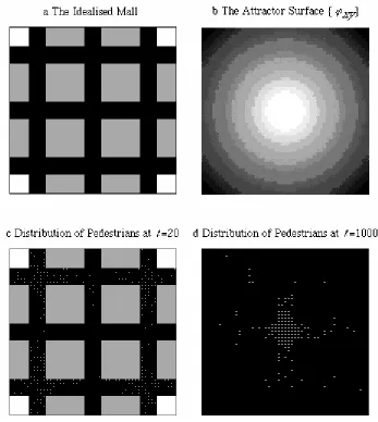
Our first example is characteristic of a planned shopping mall of the kind that

developers are locating on the edges of urban areas, particularly in North America.

The mall is square and symmetric; at each corner, there is a car park or gateway from

which shoppers enter. These gateways are connected by outer pedestrian ways which

in turn connect to the central cross routes which converge on the centre of the mall

assumed to be the prime retail pitch. Shops and other facilities are located along the

routeways. The level of spatial resolution is rather coarse based on a 51 x 51 square

grid of pixels but this was chosen to optimise speed of running the model in its

development stage. Just over half the mall is given over to pedestrian routeways: of

the 2601 pixels comprising the mall, 1305 are routeways while 1296 are retail areas

and car parks (gateways). This relatively simple geometry is shown in Figure 3(a)

although the CA software like most, treats the screen as though it is mapped onto a

opposite side and are never lost to the system. The screen wraps and in terms of this

example, there is, strictly speaking, only one pedestrian gateway for the four corners

of the screen join as one on the torus. We can remove this wrap-around feature quite

easily but we have not yet done so.

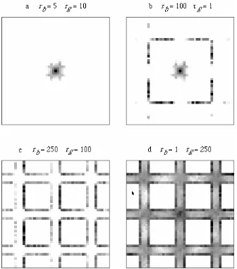
The local geometry in Figure 3(a) is complemented by a global attraction surface

{ϑxy_{} based on the relative linear accessibility to the central cell {}x y_{0 0} measured by} crow-fly distance. Then

ϑ

(24)

where Φ is a constant ensuring that the central location {x y0 0_{} is a positive value}

and the most attractive position in the system. This is shown in Figure 3(b) where it is

immediately clear that the gradient {∇ϑxy_{} is directly proportional to this unimodal} surface. Figures 3(a) and 3(b) are the two key inputs to the model; the number of

pedestrians for all these experiments has been set at 300 which is appropriate given

the scale of the example and these are randomly allocated to the four gateways prior to

the model being run. It is hard in a text to provide a real sense of the animation which

occurs as the model runs but this is important as we shall see for the paths that

walkers take are an important diagnostic to developing the model as well as important

to the realism that we seek to generate. In Figures 3(c) and (d), we show two stages in

a typical simulation; in Figure 3(c), we show a picture of walkers leaving their

gateways just after a run of the model has begun (at time t = 20) while in Figure 3(d), we show walkers converging on the central focus which is the kind of steady state that

is typical when the gradient exercises a stronger effect than the local geometry. Note

also that in Figure 3(d), the background geometry has been switched off. The program

is so configured that either the local geometry, the attraction surface, outputs such as

the density of walking so far, and the paths of walkers can be switched on or off, or

Figure 3: Local Geometry, Global Attraction and Walking in the Idealised Mall

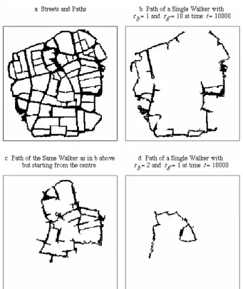
We defined various outputs from the model in the previous section where we noted

flow density surface based on {Pxyt_{} in equation (20) where the lighter tones show} higher densities and the darker lower. This is in effect a key output from the model as

it records the pattern of movement so far. In Figure 4(b), we show the path of a typical

walker in the system where the parameters have been set to make the walker move

towards the prime retail pitch which is clearly sensitive to local movement in terms of

the local geometry. At this level of resolution, we can only show a single walker but

once again, this is a useful diagnostic in showing the effect of various parameters on

the behaviour of typical walkers. In Figures 4(c) and (d) we also show another feature

of the software. Attributes associated with any agent or any location in the

environment can be examined at any point in the simulation. In Figure 4(c), we show

the key characteristics of the point x = 0, y = 2 while in 4(d) we show the attributes of the single agent (turtle 0) in the system. This can be done for any agent, any

location, and at any time in the simulation. It is a useful way of checking that

Figure 4: Typical Paths and Flow Densities

Our first tests of the model involve assessing the key feature of this framework - the

extent to which local geometry and the global attraction interact in producing

reasonable and realistic walking behaviour. To explore this, we vary the two

parameters controlling these effects - the barrier and the gradient switches τb _and τg_,

the model, we must always generate the steady state associated with each pair of

parameters τb _and τg _{and this means we must negate the returning walker effect and} any constraints on time spent in the system. In each case, we therefore examine the

patterns of movement for 300 walkers who have spent 1000 time periods in the

system. This is enough time for the steady state associated with any set of parameter

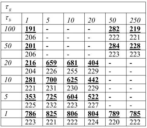
values to have emerged. The range of parameter values is shown in Figure 5 where the

combination of values used in runs of the model are indicated by the bold dots. These

values are the times when any local geometric obstacles or barriers are dealt with and

when the gradient surface is evaluated. These two effects do not cancel each other out

when applied at the same time period as the barrier effect only applies when no

progress has been made in previous time intervals. In 1000 time periods, with the

highest value for τb_{= 100, the barrier function is only invoked 10 times while with the}

largest value for τg_{= 250, the gradient is evaluated only 4 times; at these extremes,} these values have hardly any effect on the simulation.

Figure 5 shows two sets of nested designs, the first involving the area bounded by

1≤τ_b ≤100 _and 1≤τ_g ≤250

, the second by 1≤τb ≤20 _and 1≤τg ≤20_{. We have} crudely explored the larger area first. In fact, it is instructive to start with the values

(τb_{= 1,} τg_{= 1), to increment} τb _{to 100, then} τg _{to 250, then to decrement} τb _{back to}

1, and then τg _{back to 1; this is a trace around the parameter space from the bottom} left-hand corner of the grid in Figure 5 in clockwise direction. To an extent, we can

guess what is likely to happen to the walkers as we do this. At the point (τb= 1, τg= 1), walkers are always perturbed as soon as they get stuck, and they continuously set

their heading, assuming they are not stuck, in the direction of the global attraction. As

expected, walkers leave their gateways, quickly moving into the outer routeways, and

thence focusing on the central cross mall. There is, however, sufficient perturbation in

this model to make walkers who are always converging on the central point of the

mall, to move off this point. Thus although the centralising effect of these parameters

is strong, there is some circling movement around the point of central attraction. As

more significant. What happens is that walkers leave their gateways but then in their

quest to move to the centre, cling to the walls. The barrier effect is not evaluated

frequently enough to move walkers fast towards the centre. When τb _{= 100, walkers} literally creep around the walls on their way to the centre but all reach the centre

within 1000 time periods. In effect once the walkers reach the centre, they have no

incentive to move away from this and the polarisation is extremely strong. This

contains an interesting almost ‘literal’ demonstration of the idea of path dependence

(Arthur, 1988) in that although the walkers always reach the centre of the mall in the

steady state, the particular position of walkers prior to this state being reached is very

sensitive to the paths they have already taken which are determined almost entirely by