Application of a particle swarm optimization for shape
optimization in hydraulic machinery
Prokop Moravec1,a, Pavel Rudolf1
1Viktor Kaplan Dept. of Fluid Engineering, Faculty of Mechanical Engineering, Brno University of Technology, Czech Republic
Abstract.A study of shape optimization has become increasingly popular in academia and industry. A typical problem is to find an optimal shape, which minimizes (or maximizes) a certain cost function and satisfies given constraints. Particle Swarm Optimization (PSO) has received a lot of attention in past years and is inspired by social behaviour of some animals such as flocking behaviour of birds. This paper focuses on a possibility of a diffuser shape optimization using particle swarm optimization (PSO), which is coupled with CFD simulation. Influence of main parameters of PSO-algorithm and later diffuser shapes obtained with this method are discussed and advantages/disadvantages summarized.
1 Introduction
A study of size and shape optimization is very popular in industry and academia. There are a variety of methods to get the desired size/shape. These methods include nowadays well-liked particle swarm optimization (PSO) method.
This paper builds upon knowledge of an article [1] and extends the possibilities of optimizing a hydraulic diffuser, which is located behind a runner of a swirl turbine and where a recovery of kinetic energy into pressure energy takes place (Figure 1).
Fig. 1. Hydraulic turbine diffuser (dim. - metres) [1, 13]
Main goal in [1] and also in this paper is to modify the shape of the diffuser for the purpose of maximizing a coefficient of pressure recovery cp (1):
ܿൌͳଶെ ଵ
ʹ ߩݒଵଶ
ǡ (1)
where p1 (Pa) is static pressure at inlet of the
computational domain, p2 (Pa) is static pressure at outlet
of the domain; (kg/m3) is density of water, v1 (m/s) is
bulk velocity at inlet of the domain.
Note: The value of velocity at inlet is constant and does not match with the real velocity profile behind the runner of the swirl turbine [1].
2 Particle swarm optimization
Fig. 2. Particle swarm optimization – concept [14]
The PSO algorithm (PSOA) [2] was introduced in 1995 by J. Kennedy and R. Eberhart and was discovered through a simulation of a simplified social model. This algorithm is based on a bird flocking, fish schooling and swarming theory in particular.
The PSO algorithm uses a swarm of particles (subjects/individuals) randomly distributed in computational area. Individual particles exchange information about their velocity (= step size), position and fitness (fitness = solution value of the examined function).
Fig. 3. GBEST model (left) and LBEST model [7]
Each particle in PSO algorithm is treated as a point in
ܺூൌ ሺݔଵǡ ݔଶǡ ǥ ǡ ݔሻ. The best previous position of any
particle is recorded and represented as
ܲூൌ ሺଵǡ ଶǡ ǥ ǡ ሻ. The index of the best particle in
the swarm is represented by index g, and velocity for ith particle is ܸூൌ ሺݒଵǡ ݒଶǡ ǥ ǡ ݒሻ [3, 4].
There are two basic PSO concepts [3]: Global Best PSO (GBEST model) and Local Best PSO (LBEST model). They differ in swarm topology (Figure 3) [7].
In GBEST model (Figure 3) all particles are directly connected to the best solution (of the examined function) in the swarm, but on the other hand in LBEST model (Figure 3) each particle is influenced by a smaller number of neighbouring particles of the swarm array. Typically LBEST neighbourhoods consist of two neighbours, one on each side - ring lattice [7].
2.1 Global Best PSO
The particles of the swarm are moving according to the following equation [3, 4]:
ݒൌ ݒ ܿଵכ ݎܽ݊݀ሺሻ כ ሺെ ݔሻ
ܿଶכ ܴܽ݊݀ሺሻ כ ൫ െ ݔ൯,
(2)
where c1 and c2 are positive constants; rand() and Rand()
are two random vectors from range (0, 1); pgn is the best
value of the examined function obtained by the whole swarm (GBEST).
The positions of particles are afterwards computed as follows [3, 4]:
ݔൌ ݔ ݒǤ (3)
2.2 Local Best PSO
In this concept, velocity is computed similar as in Global Best PSO [3, 4]:
ݒൌ ݒ ܿଵכ ݎܽ݊݀ሺሻ כ ሺെ ݔሻ
ܿଶכ ܴܽ݊݀ሺሻ כ ሺെ ݔሻ,
(4)
only difference is pln, which is the best value of the
examined function in the particle neighbourhood (LBEST).
Note: Random vectors rand() and Rand() were later in this study (in MATLAB code) created by function rand.
3 Improvements and modifications of
Global Best PSO algorithm (PSOA)
Some references prefer Global Best PSO (pros: fast convergence, for simple problems; cons: liable to being trapped in local minimum than Local Best PSO) [3, 9, 12]. On the other hand, some references favour Local Best PSO (pros: for complex problems; cons: slower algorithm) [3, 9, 12]. In the middle stands [9] – both of
these concepts show similar performance therefore GBEST or LBEST cannot be preferred. This all leads to conclusion that the advantage of the chosen PSO mainly depends on experience of user and on the type of examined problem.
Global Best PSO algorithm is used in this paper. It can be modified in several ways for example [4, 5, 6, 7, 8]. In this study were considered only four alternations, which are mentioned in the following text.
3.1 Maximal velocity vmax
In just few iterations of PSO algorithm particle velocity can increase its value to the large magnitudes. This problem can be solved with velocity constraint – the maximal velocity vmax [8]:
ݒൌ ൜െݒݒ௫ǡ ݒ൏ െݒ௫ ௫ǡ ݒ ݒ௫
(5)
3.2 Inertia weight w
In [4] was introduced “A modified Particle Swarm Optimizer” and the inertia weight w was implemented into the equations (2, 3). Equation (2) changed to:
ݒൌ ݓ כ ݒ ܿଵכ ݎܽ݊݀ሺሻ כ ሺെ ݔሻ
ܿଶכ ܴܽ݊݀ሺሻ כ ൫ െ ݔ൯Ǥ
(6)
The inertia weight w is used to balance the global and local search abilities in the swarm. Parameter w could be treated in two possible ways: constant or adaptive.
3.2.1 Constant inertia weight w
In [4] authors suggested to choose inertia weight from interval 0.9<w<1.2 to ensure, that PSOA will have the best chance to find the global optimum (maximum of coefficient cp) in moderate number of iterations.
Authors in [8] claimed that inertia weight w=0.8 is good “starting” choice for the algorithm, but it depends mainly on the magnitude of maximal velocity vmax.
3.2.2 Adaptive inertia weight w
The inertia weight can be also computed adaptively. Many researchers have recommended that w should be large in the exploration state (the beginning of the algorithm) and small in the exploitation state (the end of the algorithm). In [5] authors proposed that w decreases linearly:
ݓ ൌ ݓ௫െ ሺݓ௫െ ݓሻ כ̴݅ݐ݁ݎܽݐ݅݊݅ݐ݁ݎܽݐ݅݊ ǡ (7)
where iteration represents current iteration of PSOA;
max_iteration represents maximal number of iterations of PSOA; wmax and wmin are maximal/minimal inertia
weights and they are usually set to 0.9 for wmax and 0.4
3.3 Parameters c1,c2
Parameter c1 represents “self-cognition”. It can maintain
diversity of the swarm (helps particle to explore computational area) [2].
Parameter c2 represents “social influence”. This
parameter forces the swarm to converge to the current global best solution of the examined function. It can also assist to the faster convergence [2].
3.3.1 Constant c1and c2
In [2] authors recommended constant values of the parameters c1 and c2 equal to integer 2. This setting
ensures that PSOA will have the best chance to find global optimum (maximum of the coefficient cp in our
case).
3.3.2 Adaptive c1and c2
Parameters c1 and c2 (c1,2 shortly) can be treated in the
same ways as inertia weight in – linearly [10]:
ܿଵൌ ൫ ܿଵെ ܿଵ൯ כ̴݅ݐ݁ݎܽݐ݅݊݅ݐ݁ݎܽݐ݅݊ ܿଵǡ (8)
and
ܿଶൌ ൫ ܿଶെ ܿଶ൯ כ̴݅ݐ݁ݎܽݐ݅݊݅ݐ݁ݎܽݐ݅݊ ܿଶǡ (9)
where iteration represents current iteration of PSOA;
max_iteration represents maximal number of iterations of PSOA; c1i and c1f are maximal/minimal values of c1
parameter and are usually set to 2.5 and 0.5 respectively;
c2i and c2f are minimal/maximal values of c2 parameter
and are usually set to 0.5 and 2.5 respectively [10].
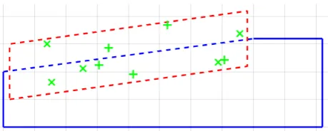
3.4 Specific computational area
In this study it was necessary to define computational area (the swarm territory) for the swarm due to possibility of creation of degenerated and inadmissible designs (geometries) – red rhomboid “FGHI” in Figure 4. If any particle emerged outside this area during the algorithm, it was immediately assigned to the relevant area border.
In this paper the computational area was built in the sufficient distance around the best solution (control point position) found in [13] – Figure 4.
Fig. 4. Specific computational area
The positions of points (x-position; y-position), which characterize computational area for the swarm, are:
F = (0.02; 0.1); G = (0.78; 0.2195); H = (0.78; 0.3195); I = (0.02; 0.3).
4 PSOA - Overview
In MATLAB software a master code was created, which calls and handles particle swarm optimization algorithm (PSOA – also programmed in MATLAB), mesh creation in Ansys ICEM CFD and CFD simulation in Ansys FLUENT.
4.1 Particle swarm optimization algorithm (PSOA)
Shape optimization using PSOA consists of several main steps (Figure 5).
Fig. 5. PSOA
For this study, the ending criterion of the algorithm was set to the maximal number of iterations (max_iteration). Initial velocities (velocity initialization – Figure 5) were set as zeros [12]. Every particle of the swarm contains information about locations of control points and value of cp and looks like this: (x1; y1; x2; y2; cp).
4.2 Computational mesh for CFD
During the shape optimization the computational 2D mesh was created in Ansys ICEM CFD. The mesh creation was handled with the text script, which ICEM can easily read and be controlled with. Mesh always met necessary quality requirements - quad type of mesh, skewness, and higher mesh resolution in near wall region (Figure 6).
4.3 CFD
Ansys FLUENT was also controlled via text script – journal. Total number of iterations was set to 1500 to ensure the adequate computational convergence. After each simulation, FLUENT saves essential variables (p1,
p2 - to the transcript file) for coefficient of pressure
recovery cp - equation (1).
Chosen discretization schemes and turbulence model were set as follows [1]:
Pressure: Standard
Momentum: Quick
Turbulent diss. rate: Second order upwind
Turbulent kinetic energy: Second order upwind ---
Turbulence model: Realizable k-
Table 1 displays types of boundary conditions, their locations (see Figure 1), magnitudes and turbulence intensity values.
Table 1. Boundary conditions [1]
Type Magnitude Turbulent
intensity
A-E Velocity
inlet
2 m/s
(constant) 5 %
B-C Pressure
outlet 0 Pa 7 %
A-B Axis - -
E-D-C Wall - -
Note: The value of velocity at inlet is constant and does not match with the real velocity profile behind the runner of the swirl turbine [1].
5 Results
5.1 Evaluation procedure
Shape change was confined to section in between points
Eand D(Figure 1). This line could be parameterized in many different ways. This study focuses only on parameterization with Bézier curves, which have two free control points (i.e. four optimization parameters).
Several test cases of chosen parameters were made (Figure 7). Every test case was repeated 5 times to capture the basic behaviour of the swarm. The ending
criterion was set to the maximal number of iterations
max_iteration=50.
Two main attributes of the swarm were examined: the magnitudes of cp of the GBEST particle (Figure 8,
10,…, 30) and the positions of the control points of the GBEST particle (Figures 9, 11,…,31).
Figure 7. Selections of the main parameters
5.2 Test cases
Initial shape
The value of coefficient of pressure recovery cp for initial
shape (Figure 1) was 0.736824 [13].
5.2.1 Swarm of 5 particles
Five particles in the swarm were chosen as the smallest reasonable number for the first six test cases. Average computational time for this choice was 28107 (s).
Free control points of Bézier curve were randomly generated in computational area at every beginning of PSOA (Figure 5). Every particle consists of two control points - one control point is represented as “x” and the other one as “+” (Figure 8).
Fig. 8. Random sets of control points – 5 particles
Note: Randomness of point generation was ensured in MATLAB by function rand. Rand returns random number from interval (0, 1).
Constant parameters w, c1,2
Figures 9 - 12 capture the examined attributes of the swarm of five particles with constant parameters w and
c1,2. The only difference between these two test cases was
a) Maximal velocity vmax=0.025
Fig. 9. Magnitudes of cp: Particles=5; w=0.8, c1,2=2; vmax=0.025
Fig. 10. Control points positions: Particles=5; w=0.8, c1,2=2;
vmax=0.025
Cp value of the GBEST particle in the swarm limited by
vmax=0.025 reached up to 0.812454.
b) Maximal velocity vmax=0.05
Fig. 11. Magnitudes of cp: Particles=5; w=0.8, c1,2=2; vmax=0.05
Fig. 12. Control points positions: Particles=5; w=0.8, c1,2=2;
vmax=0.05
This selection of parameters shows the widest spread of final values of the coefficient of pressure recovery (Figure 11). Despite this disadvantage examined function has improved compared to the initial shape. Cp value of
the GBEST particle in the swarm limited by vmax=0.05 reached up to 0.810670.
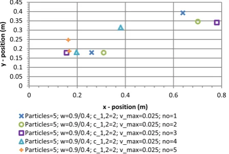
Adaptive w, constant c1,2
In these test cases only inertia weight w is adaptive – linearly decreases its value through the optimization process – equation (7). This fact should in theory help the swarm more precisely locate global maximum of cp at the
end of the PSO algorithm than the swarm with constant
w.
Figures 13 - 16 capture the examined attributes of the swarm of five particles with adaptive parameter w and constant parameters c1,2. The only difference between
these two test cases was again in maximal velocities
vmax=0.025 and vmax=0.05.
Note: Only one combination of wmax and wmin was tested
and they were set to 0.9 and 0.4 respectively. This combination was based on [4].
a) Maximal velocity vmax=0.025
Fig. 13. Magnitudes of cp: Particles=5; w=0.9/0.4, c1,2=2;
vmax=0.025
0.73 0.74 0.75 0.76 0.77 0.78 0.79 0.8 0.81 0.82
0 5 10 15 20 25 30 35 40 45 50
Cp
(1)
Iterations(1) Initialshape
Particles=5;w=0.8;c_1,2=2;v_max=0.025;no=1 Particles=5;w=0.8;c_1,2=2;v_max=0.025;no=2 Particles=5;w=0.8;c_1,2=2;v_max=0.025;no=3 Particles=5;w=0.8;c_1,2=2;v_max=0.025;no=4 Particles=5;w=0.8;c_1,2=2;v_max=0.025;no=5
0 0.050.1 0.150.2 0.250.3 0.350.4 0.45
0 0.2 0.4 0.6 0.8
y
position
(m)
x position(m) Particles=5;w=0.8;c_1,2=2;v_max=0.025;no=1 Particles=5;w=0.8;c_1,2=2;v_max=0.025;no=2 Particles=5;w=0.8;c_1,2=2;v_max=0.025;no=3 Particles=5;w=0.8;c_1,2=2;v_max=0.025;no=4 Particles=5;w=0.8;c_1,2=2;v_max=0.025;no=5
0.73 0.74 0.75 0.76 0.77 0.78 0.79 0.8 0.81 0.82
0 5 10 15 20 25 30 35 40 45 50
Cp
(1)
Iterations(1) Initialshape
Particles=5;w=0.8;c_1,2=2;v_max=0.05;no=1 Particles=5;w=0.8;c_1,2=2;v_max=0.05;no=2 Particles=5;w=0.8;c_1,2=2;v_max=0.05;no=3 Particles=5;w=0.8;c_1,2=2;v_max=0.05;no=4 Particles=5;w=0.8;c_1,2=2;v_max=0.05;no=5
0 0.050.1 0.150.2 0.250.3 0.350.4 0.45
0 0.2 0.4 0.6 0.8
y
position
(m)
x position(m) Particles=5;w=0.8;c_1,2=2;v_max=0.05;no=1 Particles=5;w=0.8;c_1,2=2;v_max=0.05;no=2 Particles=5;w=0.8;c_1,2=2;v_max=0.05;no=3 Particles=5;w=0.8;c_1,2=2;v_max=0.05;no=4 Particles=5;w=0.8;c_1,2=2;v_max=0.05;no=5
0.73 0.74 0.75 0.76 0.77 0.78 0.79 0.8 0.81 0.82
0 5 10 15 20 25 30 35 40 45 50
Cp
(1)
Iterations(1) Initialshape
Fig. 14. Control points positions: Particles=5; w=0.9/0.4, c1,2=2;
vmax=0.025
Cp value of the GBEST particle in the swarm limited by
vmax=0.025 reached up to 0.812733.
b) Maximal velocity vmax=0.05
Fig. 15. Magnitudes of cp: Particles=5; w=0.9/0.4, c1,2=2;
vmax=0.05
Fig. 16. Control points positions: Particles=5; w=0.9/0.4, c1,2=2;
vmax=0.05
Cp value of the GBEST particle in the swarm limited by
vmax=0.05 reached up to 0.812915.
Adaptive parameters w, c1,2
The last two test cases contain swarms with adaptive parameters w and c1,2. The modification of these
parameters was realized via linear decrease – equations (7, 8, 9). This combination of parameters forces the swarm to quick convergence to the global maximum of cp, but one danger could emerge – convergence to some
local minimum without proper “search” of the computational area.
Figures 17 - 20 capture the examined attributes of the swarm of five particles with adaptive parameter w and adaptive parameters c1,2. The only difference between
these two test cases was once again in maximal velocities
vmax=0.025 and vmax=0.05.
Note: Only one combination of wmax, wmin [4] and one
combination of maximal/minimal values of c1/c2 [10] was
tested.
a) Maximal velocity vmax=0.025
Fig. 17. Magnitudes of cp: Particles=5; w=0.9/0.4, c1,2=2.5/0.5;
vmax=0.025
Fig. 18. Control points positions: Particles=5; w=0.9/0.4, c1,2=2;
vmax=0.025
Cp value of the GBEST particle in the swarm limited by
vmax=0.025 reached up to 0.812733.
0 0.050.1 0.150.2 0.250.3 0.350.4 0.45
0 0.2 0.4 0.6 0.8
y
position
(m)
x position(m) Particles=5;w=0.9/0.4;c_1,2=2;v_max=0.025;no=1 Particles=5;w=0.9/0.4;c_1,2=2;v_max=0.025;no=2 Particles=5;w=0.9/0.4;c_1,2=2;v_max=0.025;no=3 Particles=5;w=0.9/0.4;c_1,2=2;v_max=0.025;no=4 Particles=5;w=0.9/0.4;c_1,2=2;v_max=0.025;no=5
0.73 0.74 0.75 0.76 0.77 0.78 0.79 0.8 0.81 0.82
0 5 10 15 20 25 30 35 40 45 50
Cp
(1)
Iterations(1) Initialshape
Particles=5;w=0.9/0.4;c_1,2=2;v_max=0.05;no=1 Particles=5;w=0.9/0.4;c_1,2=2;v_max=0.05;no=2 Particles=5;w=0.9/0.4;c_1,2=2;v_max=0.05;no=3 Particles=5;w=0.9/0.4;c_1,2=2;v_max=0.05;no=4 Particles=5;w=0.9/0.4;c_1,2=2;v_max=0.05;no=5
0 0.050.1 0.150.2 0.250.3 0.350.4 0.45
0 0.2 0.4 0.6 0.8
y
position
(m)
x position(m) Particles=5;w=0.9/0.4;c_1,2=2;v_max=0.05;no=1 Particles=5;w=0.9/0.4;c_1,2=2;v_max=0.05;no=2 Particles=5;w=0.9/0.4;c_1,2=2;v_max=0.05;no=3 Particles=5;w=0.9/0.4;c_1,2=2;v_max=0.05;no=4 Particles=5;w=0.9/0.4;c_1,2=2;v_max=0.05;no=5
0.73 0.74 0.75 0.76 0.77 0.78 0.79 0.8 0.81 0.82
0 5 10 15 20 25 30 35 40 45 50
Cp
(1)
Iterations(1) Initialshape
Particles=5;w=0.9/0.4;c_1,2=2.5/0.5;v_max=0.025;no=1 Particles=5;w=0.9/0.4;c_1,2=2.5/0.5;v_max=0.025;no=2 Particles=5;w=0.9/0.4;c_1,2=2.5/0.5;v_max=0.025;no=3 Particles=5;w=0.9/0.4;c_1,2=2.5/0.5;v_max=0.025;no=4 Particles=5;w=0.9/0.4;c_1,2=2.5/0.5;v_max=0.025;no=5
0 0.050.1 0.150.2 0.250.3 0.350.4 0.45
0 0.2 0.4 0.6 0.8
y
position
(m)
x position(m)
b) Maximal velocity vmax=0.05
Fig. 19. Magnitudes of cp: Particles=5; w=0.9/0.4, c1,2=2.5/0.5;
vmax=0.05
Fig. 20. Control points positions: Particles=5; w=0.9/0.4, c1,2=2;
vmax=0.025
Cp value of the GBEST particle in the swarm limited by
vmax=0.05 reached up to 0.812543.
Partial results
Every test case improved the value of the coefficient cp
compared to the initial shape – Table 2. The best diffuser design is shown in Figure 21.
For constant parameters w and c1,2 is better choice
smaller maximal velocity vmax=0.025. This fact strongly
depends on the size of computational area for the swarm. On the other hand - when at least one of the parameter is adaptive, the bigger maximal velocity (vmax=0.05) seems
to be a good choice to achieve better results.
Test case with adaptive w and c1,2 shows the most
stable values of the coefficient cp (Figure 19), on the
other hand the most unstable test case was with parameters w=0.8; c1,2=2; vmax=0.05 (Figure 10).
The disadvantage of each test case is in final positions of the control points of Bézier curves – in every single test they were spread out across the whole computational area and they never converged to a specific location.
Table 2. Partial results of 5-particle swarm
5 particles
Parameter selection Best cp (1)
w=0.8; c1,2=2; vmax=0.025 (no. 5) 0.812454
w=0.8; c1,2=2; vmax=0.05 (no. 4) 0.810670
w=0.9/0.4; c1,2=2; vmax=0.025 (no. 5) 0.812733
w=0.9/0.4; c1,2=2; vmax=0.05 (no. 3) – Figure 21. 0.812915
w=0.9/0.4; c1,2=2.5/0.5; vmax=0.025 (no. 5) 0.812733
w=0.9/0.4; c1,2=2.5/0.5; vmax=0.05 (no.4) 0.812543
Note: The coefficient of pressure recovery cp increases as
a result of weaker velocity gradients and shear layers (it was confirmed by theoretical analysis in [11]).
Fig. 21. The best diffuser design achieved by swarm of five
5.2.2 Swarm of 10 particles
The last six test cases contain swarms of ten particles. Average computational time of this choice was 56925 (s).
Once again: Free control points of Bézier curve were randomly generated in computational area at every beginning of PSOA (Figure 5). Every particle consists of two control points - one control point is represented as “x” and the other one as “+” (Figure 22).
Fig. 22. Random sets of control points in computational area – 10 particles
Note: Swarms with larger number of particles were not tested due to enormous size of computational time.
Test procedure was the same as in case of swarm of five – evaluation technique was executed according to the diagram in Figure 7.
0.73 0.74 0.75 0.76 0.77 0.78 0.79 0.8 0.81 0.82
0 5 10 15 20 25 30 35 40 45 50
Cp
(1)
Iterations(1) Initialshape
Particles=5;w=0.9/0.4;c_1,2=2.5/0.5;v_max=0.05;no=1 Particles=5;w=0.9/0.4;c_1,2=2.5/0.5;v_max=0.05;no=2 Particles=5;w=0.9/0.4;c_1,2=2.5/0.5;v_max=0.05;no=3 Particles=5;w=0.9/0.4;c_1,2=2.5/0.5;v_max=0.05;no=4 Particles=5;w=0.9/0.4;c_1,2=2.5/0.5;v_max=0.05;no=5
0 0.050.1 0.150.2 0.250.3 0.350.4 0.45
0 0.2 0.4 0.6 0.8
y
position
(m)
x position(m)
Constant parameters w, c1,2
a) Maximal velocity vmax=0.025
Fig. 23. Magnitudes of cp: Particles=10; w=0.8, c1,2=2;
vmax=0.025
Fig. 24. Control points positions: Particles=10; w=0.8, c1,2=2;
vmax=0.025
Cp value of the GBEST particle in the swarm limited by
vmax=0.025 reached up to 0.812857.
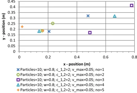
b) Maximal velocity vmax=0.05
Fig. 25. Control points positions: Particles=10; w=0.8, c1,2=2;
vmax=0.05
Fig. 26. Control points positions: Particles=10; w=0.8, c1,2=2;
vmax=0.05
Cp value of the GBEST particle in the swarm limited by
vmax=0.05 reached up to 0.812707.
Adaptive w, constant c1,2
a) Maximal velocity vmax=0.025
Fig. 27. Magnitudes of cp: Particles=10; w=0.9/0.4, c1,2=2;
vmax=0.025
Fig. 28. Control points positions: Particles=10; w=0.9/0.4, c1,2=2; vmax=0.025
Cp value of the GBEST particle in the swarm limited by
vmax=0.025 reached up to 0.812698.
0.73 0.74 0.75 0.76 0.77 0.78 0.79 0.8 0.81 0.82
0 5 10 15 20 25 30 35 40 45 50
Cp
(1)
Iterations(1) Initialshape
Particles=10;w=0.8;c_1,2=2;v_max=0.025;no=1 Particles=10;w=0.8;c_1,2=2;v_max=0.025;no=2 Particles=10;w=0.8;c_1,2=2;v_max=0.025;no=3 Particles=10;w=0.8;c_1,2=2;v_max=0.025;no=4 Particles=10;w=0.8;c_1,2=2;v_max=0.025;no=5
0 0.050.1 0.150.2 0.250.3 0.350.4 0.45
0 0.2 0.4 0.6 0.8
y
position
(m)
x position(m) Particles=10;w=0.8;c_1,2=2;v_max=0.025;no=1 Particles=10;w=0.8;c_1,2=2;v_max=0.025;no=2 Particles=10;w=0.8;c_1,2=2;v_max=0.025;no=3 Particles=10;w=0.8;c_1,2=2;v_max=0.025;no=4 Particles=10;w=0.8;c_1,2=2;v_max=0.025;no=5
0.73 0.74 0.75 0.76 0.77 0.78 0.79 0.8 0.81 0.82
0 5 10 15 20 25 30 35 40 45 50
Cp
(1)
Iterations(1) Initialshape
Particles=10;w=0.8;c_1,2=2;v_max=0.05;no=1 Particles=10;w=0.8;c_1,2=2;v_max=0.05;no=2 Particles=10;w=0.8;c_1,2=2;v_max=0.05;no=3 Particles=10;w=0.8;c_1,2=2;v_max=0.05;no=4 Particles=10;w=0.8;c_1,2=2;v_max=0.05;no=5
0 0.050.1 0.150.2 0.250.3 0.350.4 0.45
0 0.2 0.4 0.6 0.8
y
position
(m)
x position(m) Particles=10;w=0.8;c_1,2=2;v_max=0.05;no=1 Particles=10;w=0.8;c_1,2=2;v_max=0.05;no=2 Particles=10;w=0.8;c_1,2=2;v_max=0.05;no=3 Particles=10;w=0.8;c_1,2=2;v_max=0.05;no=4 Particles=10;w=0.8;c_1,2=2;v_max=0.05;no=5
0.73 0.74 0.75 0.76 0.77 0.78 0.79 0.8 0.81 0.82
0 5 10 15 20 25 30 35 40 45 50
Cp
(1)
Iterations(1) Initialshape
Particles=10;w=0.9/0.4;c_1,2=2;v_max=0.025;no=1 Particles=10;w=0.9/0.4;c_1,2=2;v_max=0.025;no=2 Particles=10;w=0.9/0.4;c_1,2=2;v_max=0.025;no=3 Particles=10;w=0.9/0.4;c_1,2=2;v_max=0.025;no=4 Particles=10;w=0.9/0.4;c_1,2=2;v_max=0.025;no=5
0 0.050.1 0.150.2 0.250.3 0.350.4 0.45
0 0.2 0.4 0.6 0.8
y
position
(m)
x position(m)
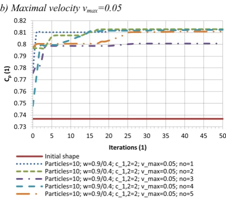
b) Maximal velocity vmax=0.05
Fig. 29. Magnitudes of cp: Particles=10; w=0.9/0.4, c1,2=2;
vmax=0.05
Fig. 30. Control points positions: Particles=10; w=0.9/0.4, c1,2=2; vmax=0.05
Cp value of the GBEST particle in the swarm limited by
vmax=0.05 reached up to 0.812831.
Adaptive parameters w, c1,2
a) Maximal velocity vmax=0.025
Fig. 31. Magnitudes of cp: Particles=10; w=0.9/0.4, c1,2=2.5/0.5;
vmax=0.025
Fig. 32. Control points positions: Particles=10; w=0.9/0.4, c1,2=2; vmax=0.025
a) Maximal velocity vmax=0.05
Fig. 33. Magnitudes of cp: Particles=10; w=0.9/0.4, c1,2=2.5/0.5;
vmax=0.05
Fig. 34. Control points positions: Particles=10; w=0.9/0.4, c1,2=2; vmax=0.05
0.73 0.74 0.75 0.76 0.77 0.78 0.79 0.8 0.81 0.82
0 5 10 15 20 25 30 35 40 45 50
Cp
(1)
Iterations(1) Initialshape
Particles=10;w=0.9/0.4;c_1,2=2;v_max=0.05;no=1 Particles=10;w=0.9/0.4;c_1,2=2;v_max=0.05;no=2 Particles=10;w=0.9/0.4;c_1,2=2;v_max=0.05;no=3 Particles=10;w=0.9/0.4;c_1,2=2;v_max=0.05;no=4 Particles=10;w=0.9/0.4;c_1,2=2;v_max=0.05;no=5
0 0.050.1 0.150.2 0.250.3 0.350.4 0.45
0 0.2 0.4 0.6 0.8
y
position
(m)
x position(m) Particles=10;w=0.9/0.4;c_1,2=2;v_max=0.05;no=1 Particles=10;w=0.9/0.4;c_1,2=2;v_max=0.05;no=2 Particles=10;w=0.9/0.4;c_1,2=2;v_max=0.05;no=3 Particles=10;w=0.9/0.4;c_1,2=2;v_max=0.05;no=4 Particles=10;w=0.9/0.4;c_1,2=2;v_max=0.05;no=5
0.73 0.74 0.75 0.76 0.77 0.78 0.79 0.8 0.81 0.82
0 5 10 15 20 25 30 35 40 45 50
Cp
(1)
Iterations(1) Initialshape
Particles=10;w=0.9/0.4;c_1,2=2.5/0.5;v_max=0.025;no=1 Particles=10;w=0.9/0.4;c_1,2=2.5/0.5;v_max=0.025;no=2 Particles=10;w=0.9/0.4;c_1,2=2.5/0.5;v_max=0.025;no=3 Particles=10;w=0.9/0.4;c_1,2=2.5/0.5;v_max=0.025;no=4 Particles=10;w=0.9/0.4;c_1,2=2.5/0.5;v_max=0.025;no=5
0 0.050.1 0.150.2 0.250.3 0.350.4 0.45
0 0.2 0.4 0.6 0.8
y
position
(m)
x position(m)
Particles=10;w=0.9/0.4;c_1,2=2.5/0.5;v_max=0.025;no=1 Particles=10;w=0.9/0.4;c_1,2=2.5/0.5;v_max=0.025;no=2 Particles=10;w=0.9/0.4;c_1,2=2.5/0.5;v_max=0.025;no=3 Particles=10;w=0.9/0.4;c_1,2=2.5/0.5;v_max=0.025;no=4 Particles=10;w=0.9/0.4;c_1,2=2.5/0.5;v_max=0.025;no=5
0.73 0.74 0.75 0.76 0.77 0.78 0.79 0.8 0.81 0.82
0 5 10 15 20 25 30 35 40 45 50
Cp
(1)
Iterations(1) Initialshape
Particles=10;w=0.9/0.4;c_1,2=2.5/0.5;v_max=0.05;no=1 Particles=10;w=0.9/0.4;c_1,2=2.5/0.5;v_max=0.05;no=2 Particles=10;w=0.9/0.4;c_1,2=2.5/0.5;v_max=0.05;no=3 Particles=10;w=0.9/0.4;c_1,2=2.5/0.5;v_max=0.05;no=4 Particles=10;w=0.9/0.4;c_1,2=2.5/0.5;v_max=0.05;no=5
0 0.050.1 0.150.2 0.250.3 0.350.4 0.45
0 0.2 0.4 0.6 0.8
y
position
(m)
x position(m)
Partial results
Every test case improved the value of cp coefficient
compared to the initial shape – Table 3. The design of the best attempt is shown in Figure 35.
Trend of smaller maximal velocity for constant parameters continues also for the swarms of ten particles – Figure 23.
Ten particles should generally search the computational area thoroughly (compared to five particles), but the highest value of cp falls behind the swarms of five (for
comparison Tables 2 and 3).
The disadvantage of almost every test case is in final positions of the control points of Bézier curves, but compared to the swarms of 5 particles, there is a promising combination of parameters w=0.9/0.4;
c1,2=2.5/0.5; vmax=0.025 – see Figures 31 and 32. This
combination shows stable cp values and stable positions
of control points in the end of the test; on the other hand this test case converged to some local maximum and did not bring the highest value of the examined function (coefficient of cp).
Table 3. Partial results of 10-particle swarm
10 particles
Parameter selection Best cp (1)
w=0.8; c1,2=2; vmax=0.025 (no. 2) – Figure 35. 0.812857
w=0.8; c1,2=2; vmax=0.05 (no. 5) 0.812707
w=0.9/0.4; c1,2=2; vmax=0.025 (no. 5) 0.812698
w=0.9/0.4; c1,2=2; vmax=0.05 (no. 2). 0.812831
w=0.9/0.4; c1,2=2.5/0.5; vmax=0.025 (no. 3) 0.812530
w=0.9/0.4; c1,2=2.5/0.5; vmax=0.05 (no.3) 0.812563
Note: The coefficient of pressure recovery cp increases as
a result of weaker velocity gradients and shear layers (it was confirmed by theoretical analysis in [11]).
Fig. 35. Best diffuser design achieved by swarm of ten
6 Conclusions
Particle Swarm Optimization (PSO) is quite interesting and productive non-gradient type of optimization, which
is based on social behaviour of various animals and uses swarm of particles to find global optimum.
Application of this optimization method strongly depends on examined problem. Present paper builds upon knowledge of [1] and focuses its energy on optimization of the hydraulic turbine diffuser. The shape optimization of the turbine diffuser became a basic model prototype of various methods [1, 13].
Two types of swarms were constructed – with five and ten particles and with different combinations of parameters (Figure 7). Every time PSO managed to improve value of cp compared to the initial shape (Figure
1) - cp increases as a result of weaker velocity gradients
and shear layers. Final diffuser designs (Figure 21 and 35) had similar shape and achieved similar cp -0.812915
for swarm of five and 0.812857 for the swarm of ten particles.
The main advantage of PSO: high value of coefficient of pressure recovery, because particles can “search” the computational area quite effectively. But on the other hand there are also some disadvantages: a need of creation of the computational area (Figure 4) to avert of production of degenerated designs and also a computational time was an issue – every iteration a great number of CFD simulation had to be performed.
Overall the PSO shows promising results – Table 4.
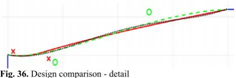
Table 4. Comparison of optimization methods
Method cp (1)
Adjoint solver- 4. order
polynomial [1] 0.812354 dotted line
Nelder-Mead – Bézier curve
with 2 free control points [13] 0.812146
dashed line (with “o”) Particle Swarm Optimization -
Bézier curve with 2 free control points
0.812915 solid line
(with “x”)
It shows that the PSO algorithm produced slightly better values of cp than both Nelder-Mead algorithm and
Adjoint solver.
Control points positions do not match, when PSO and Nelder-Mead are compared – Figure 36. But in general – all three methods show similar foundation of the final design – the tapered shape at the inlet of the diffuser and thus the crucial difference lies in the rest of the parametrized curve (Figure 36).
Fig. 36. Design comparison - detail
There are some ways for improvement - future work will focus on some possible modifications of PSO e.g.:
1. Particle reduction during the algorithm – exploit a benefit of a large number of particles at the beginning of the algorithm and then if a certain criterion is met, algorithm will start to reduce the size of the swarm. This alternation brings potential savings in the computational time. 2. Combination of two optimization methods – at
the beginning of the optimization process usage of PSO for its robustness and later in the end of the process an application of a straight forward method as Nelder-Mead to ensure good convergence. Also this modification brings potential savings in computational time.
References
1. P. Moravec, J. Hliník, P. Rudolf: Optimization of Hydraulic Turbine Diffuser. EFM 2015, Prague, 2015, pp. 1-7.
2. J. Kennedy, R. Eberhart: Particle swarm
optimization. The IEEE International Conference on Neural Networks, Perth, 1995, vol. 4, pp. 1942-1948. 3. J. Kennedy, R. Eberhart: A new Optimizer Using
Particles Swarm Theory. The Sixth International Symposium on Micro Machine and Human Science, Nagoya, 1995, pp. 39-43.
4. Y. H. Shi, R. Eberhart: A Modified Particle Swarm Optimizer. The Int. Conf. on Evolutionary Computation, 1998, pp. 69-73.
5. Y. H. Shi, R. Eberhart: Empirical Study of Particle Swarm Optimization. IEEE 1999, pp. 1945-1950.
6. Z.-H. Zhan, J. Zhang, Y. Li, H. S.-H. Chung:
Adaptive Particle Swarm Optimization. The IEEE Transactions on Systems, Man, and Cybernetics, 2009, vol. 39, pp. 1362-1381.
7. J. Kennedy, R. Mendes: Population Structure and Particle Swarm Performance. Proceedings of the Evolutionary Computation 2002, vol. 2, pp. 1671-1676.
8. Y. H. Shi, R. Eberhart: Parameter Selection in Particle Swarm Optimization. Evolutionary Programming VII: Proceedings of the Seventh Annual Conference on Evolutionary programming, San Diego, 1998, pp. 591-600.
9. A.P. Engelbrecht: Particle swarm optimization: Global or Local Best? BRICKS Congress on Computational Intelligence and 11th Brazilian Congress on Computational Intelligence 2013, pp. 124-135.
10. A. Ratnaweera, S. K. Halgamuge, H.C. Watson: Self-organizing hierarchical particle swarm optimizer with time-varying acceleration coefficients. IEEE Transactions on Evolutionary Computation 2004, pp. 240-255.
11. P. Rudolf: Study of the shear layers for swirl draft tube optimization. PhD thesis. In Czech
12. A.P. Engelbrecht: Particle Swarm Optimization: Velocity initialization. IEEE World Congress on Computational Intelligence, Brisbane, 2012.
13. J. Hliník: Shape optimization of hydraulic turbine diffuser. Bachelor thesis. In Slovak. 2015, Brno. 14. Conceptual diagram of PSO in action with a single
global minimum. Figure : PSO_concept.png
[online] [cit 2016-09-01]. Available online : http://wirelesstechthoughts.blogspot.cz/2013/06/an-introduction-to-particle-swarm.html