Experimental determination of the heat transfer coefficient in shell-and-tube condensers using the Wilson plot method

Experimental determination of the heat transfer coefficient in

shell-and-tube condensers using the Wilson plot method

Jan Havlik1,*, Tomas Dlouhy1

1_{Czech Technical University in Prague, Faculty of Mechanical Engineering, Department of Energy Engineering,, Technicka 4,} 16607 Prague 6, Czech Republic

Abstract. This article deals with the experimental determination of heat transfer coefficients. The calculation of heat transfer coefficients constitutes a crucial issue in design and sizing of heat exchangers. The Wilson plot method and its modifications based on measured experimental data utilization provide an appropriate tool for the analysis of convection heat transfer processes and the determination of convection coefficients in complex cases. A modification of the Wilson plot method for shell-and-tube condensers is proposed. The original Wilson plot method considers a constant value of thermal resistance on the condensation side. The heat transfer coefficient on the cooling side is determined based on the change in thermal resistance for different conditions (fluid velocity and temperature). The modification is based on the validation of the Nusselt theory for calculating the heat transfer coefficient on the condensation side. A change of thermal resistance on the condensation side is expected and the value is part of the calculation. It is possible to improve the determination accuracy of the criterion equation for calculation of the heat transfer coefficient using the proposed modification. The criterion equation proposed by this modification for the tested shell-and-tube condenser achieves good agreement with the experimental results and also with commonly used theoretical methods.

1 Introduction

The heat transfer mechanism by convection is an energy transfer between a solid surface and a moving fluid induced by a temperature difference between the solid surface and the fluid. Heat transfer by convection is indeed a combination of conduction and fluid motion. The analytical treatment of convection problems requires the solution of a system of mass, momentum and energy conservation equations. Although these procedures are elaborate, analytic solutions are available for simple geometries under restrictive assumptions. Most of the convective heat transfer processes inherent to heat exchangers usually involve complex geometries and complicated flows so analytical solutions are not possible. Therefore, an approach based on Newton’s law of cooling (see Eq. (1)), provides a simple alternate technique. Newton’s law of cooling established an algebraic relation between the heat flow by convectionܳ, the surface areaܣ, the heat transfer coefficient ݄ and the temperature difference between the solid surface ܶ௦and the fluid ܶ௙ .

ܳ ൌ ݄ ή ൫ܶ௙െ ܶ௦൯ ή ܣ (1)

For a given flow and surface geometry, the experimental data is usually obtained by measuring the surface and fluid temperatures. Then the heat transfer coefficient (HTC) may be calculated from Eq. (1).

However, the main difficulty of this methodology lies in the measurement of the surface temperature, because the surface temperature varies from point to point, and the flow profile could be altered by the presence of the temperature sensors. Moreover, in many cases of heat exchangers the heat transfer surface is not accessible. Therefore, any alternative method conducive to the HTC calculation is attractive because of widespread use and practical applications [1].

2 Wilson plot method

The Wilson plot method is used for the experimental determination of the HTC or coefficients of a criterion equation, which describes the HTC calculation. This method avoids the direct measurement of the surface temperature and consequently any disturbance of the fluid flow and heat transfer introduced while attempting to measure those temperatures. Therefore, the method constitutes a suitable technique for estimating HTCs in a variety of convective heat transfer processes [1].

manner [1]. This method was originally derived for determining the coolant HTC in steam condensers where steam condenses outside the tubes and the coolant flows inside. The sensitivity of the coolant HTC value to the overall HTC is more significant than the condensation HTC [2]. The mean value of the HTC on the coolant side can be described as a function of the speed of the coolant [1].

The aim of the method is to calculate the convection coefficients (or thermal resistance) of the fluid in the criterion equation for the defined type of convection heat transfer. Modifications of the Wilson plot method were proposed to enhance its accuracy. The principle of the original method is still maintained. The application of the Wilson plot method is based on the measurement of the experimental mass flow rate and temperatures.

3 Tested heat exchanger

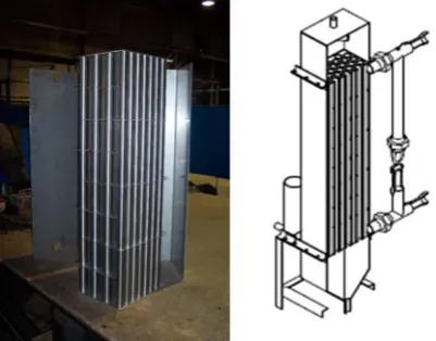
The tested heat exchanger is a vertical shell-and-tube model in which the condensing water vapour flows downwards inside vertical tubes and the cooling water flows in a counter current in the outer shell (see Fig. 1). The shell side has a complex geometry with complicated flow patterns so using the Wilson plot method is suitable for determining the shell-side HTC.

The tube bundle is formed by 49 tubes 865 mm in length, 28 mm in external diameter and 24 mm in internal diameter. The tubes are arranged in staggered arrays with a triangular tube pitch of 35 mm. The cross-section of the shell is rectangular in shape, 223 mm by 270 mm in size. Seven segmental baffles (223 x 230 mm) are used in the shell section. The tubes are made from stainless steel 1.4301 (AISI 304).

Fig. 1. Vertical tube condenser

The testing loop is shown in Fig. 2. Steam is produced in a steam generator. Before the steam enters the vertical tube condenser, its parameters are reduced to the required values. Hot water recirculation enables the cooling water temperature and the cooling water flow rate in the condenser to be regulated. The measured parameters are the inlet cooling water temperature ܶ_௪ଵ, the temperature of the water after recirculation ܶ௪ଶ, the

outlet cooling water temperature ܶ_௪ଷ, the cooling water flow rate ܳ௪, the inlet steam pressure ݌௦ , the inlet

steam temperature ܶ_௦ and the amount of steam condensate ܯ௖.

Fig. 2. Scheme of the testing loop

4 Original Wilson Plot method

Derivation of the Wilson-plot is well described in [1]. The overall thermal resistance of the condensation process in a shell-and-tube condenser ܴ_௢௩ can be expressed as the sum of three thermal resistances corresponding to the internal convectionܴ_௜, the tube wall ܴ_௦ and the external convection ܴ_௢ as

ܴ௢௩ൌ ܴ௜ ൅ܴ௦൅ܴ௢ (2)

For the sake of simplicity, the thermal resistances of the fluid fouling are neglected. Wilson theorized that if the mass flow of the cooling liquid was modified, then the change in the overall thermal resistance would be mainly due to the variation of the coolant HTC, while the remaining thermal resistances remained nearly constant. The HTC varies with the fluid mass flow for many cases of the convection heat transfer process excluding the phase changes. It is valid also for complex heat exchanger geometries. An illustrative example of the experimental determined dependence of the HTC on the fluid mass flow is well described in [3].

Therefore, the thermal resistances on the condensation side and the tube wall could be considered constant. In the case of a condenser where steam condenses inside the tubes is considered

ܴ௜ ൅ ܴ௦ ൌ ܥଵ (3)

where ܥ_ଵis a constant. For the thermal resistance on the cooling water side ܴ_௢is considered

ܴ௢ൌ _݄ܣͳ (4)

where ܣis the heat surface area and the HTC on the cooling water side ݄ is proportional to the power of the fluid velocity ݒ

݄ ൌ ܥଶή ݒ௡ (5)

Upon combining Eq. (2), Eq. (3), Eq. (4) and Eq. (5), the overall thermal resistance turns out to be a linear function of ݒ௡

ܴ௢௩ൌ_ܥͳ ଶܣή

ͳ

ݒ௡൅ ܥଵ (6)

This is presented graphically in Fig. 3.

Fig. 3. A linear function of the thermal resistance [1]

From here, the straight line equation that fits the experimental data can be deduced by applying simple linear regression. The overall thermal resistance may be expressed as a function of the overall heat transfer coefficient ܷ and surface area ܣ

ܴ௢௩ൌ_{ܷ ή ܣ}ͳ (7)

Then, for each set of experimental data corresponding to each mass flow rate, the overall thermal resistance is provided by substituting Eq. (7) to Eq. (7). This equation describes the calculation of the overall heat transfer coefficient from the performance of the heat exchanger and the logarithmic mean temperature difference of the fluids ߂ܶ_௟௢௚

ܷ ൌ_{ܣ ή ߂ ܶ}ܳ

௟௢௚ (8)

The heat exchanger performance ܳ is provided by the equation

ܳ ൌ ܯ௪ήܿ௪ή൫ܶ௪ǡ௢௨௧െܶ௪ǡ௜௡൯ (9)

where ܯ_௪ is the cooling water flow, ܿ_௪is the specific heat capacity of water, ܶ_{௪ǡ௢௨௧} is the outlet cooling water temperature and ܶ_௪ǡ௜௡ is the inlet cooling water temperature [1].

5 Proposed modification of the Wilson

plot method

The determination of the HTC on the cooling side is based on the change in thermal resistance for different conditions (fluid velocity and temperature). The modification considers the presumption of validity of the

Nusselt theory for calculation of the HTC on the condensation side. The thermal resistance on the condensation side varies and it is part of the calculation.

5.1 Non-dimensional parameters of the heat exchangers

Reynolds Number

The Reynolds number ܴ݁ is a function of the fluid flow rate. The mathematical formula for the Reynolds number is provided in Eq. (10). The ratio represents momentum to viscous forces, where ݒ is the fluid velocity, ܦ is characteristic diameter and ߥ is the kinematic viscosity [4].

ܴ݁ ൌݒ ή ܦ_ߥ (10)

Prandtl Number

The Prandtl number ܲݎ is a function of two important physical properties (thermal and momentum). The Prandtl number may be seen as the ratio of the rate that viscous forces penetrate the material to the rate that thermal energy penetrates the material [4]. In Eq. (11), ߤ is the dynamic viscosity, ܿ_௣ the material heat capacity and ݇ is thermal conductivity.

ܲݎ ൌߤ ή ܿ_݇ ௣ (11)

Nusselt Number

The Nusselt number ܰݑ is equal to the dimensionless temperature gradient at the surface and it essentially provides a measure of the convective heat transfer. The Nusselt number may be viewed as the ratio of the conduction resistance of a material to the convection resistance of the same material [4].

ܰݑ ൌ݄ ή ܦ_݇ (12)

Nusselt Number Correlations

In single phase fluid flow heat transfer, the Nusselt number is generally represented by a pragmatic expression in the form as seen in (13). The term (ȝ/ȝs) is

accountable for the variable viscosity effect for the case that the viscosity varies from the centre of the tube towards the tube wall [4].

ܰݑ ൌ ܥ ή ܴ݁௡_{ή ܲݎ}௠_{ή ൬}ߤ

ߤ௦൰ ଴Ǥଵସ

(13)

5.2 Derivation of the proposed modification

ܴ௢௩ൌ_݄ ͳ ௖ή ܣ௜൅

݈݊ሺ݀௢Τ ሻ݀௜

ʹ ή ߨ ή ݇௧ή ܮ௧൅

ͳ

݄௪ή ܣ௢ (14)

where ݄_௖and ݄_௪are the condensation and cooling water HTCs, ݀_௜ and ݀_௢ are the inner and outer tube diameters, ݇௧is the tube thermal conductivity, ܮ௧is the tube length

and ܣ_௜and ܣ_௢are the inner and outer tube surface areas, respectively. By combining Eq. (8) and (14) is given

ͳ ܷ ή ܣൌ

ͳ ݄௖ή ܣ௜൅

݈݊ሺ݀௢Τ ሻ݀௜

ʹ ή ߨ ή ݇௧ή ܮ௧൅

ͳ

݄௪ή ܣ௢ (15)

where݄_௪, can be expressed combining Eq. (12) and (13)

݄௪ൌ݇_ܦ௪ή ܥ ή ܴ݁௡ή ܲݎ௠ή ൬_ߤߤ ௦൰

଴Ǥଵସ

(16)

and ݄_௖ is defined by the Nusselt condensation theory [5], [6] as

݄௖ ൌ ͲǤͻͶ͵ ቈߩ௅݃൫ߩ௅െ ߩ௣൯݄௙௚ ᇱ _݇

௅ଷ

ߤ௅οܶ௦௔௧ܮ ቉ ଵ ସΤ

(17)

where ߩ_௅is the density of the condensate, ߩ_௣is the density of the water vapour, ݄_௙௚ᇱ is the latent heat of condensation, ݇_௅ is the thermal conductivity of the condensate, ߤ_௅ is the dynamic viscosity of the condensate, οܶ_௦௔௧ is the saturation and wall temperature difference, ܮ is the wall length. By a substitution of terms in (8) and (16) to equation (15) is given

ͳ

൬_{ܣ ή ߂ ܶ}ܳ

௟௢௚൰ ή ܣ

ൌ ͳ

݄௖ή ܣ௜൅

݈݊ሺ݀௘Τ ሻ݀௜

ʹ ή ߨ ή ߣ௦ή ܮ௦

൅_݇ ͳ

௪

ܦ ή ܥ ή ܴ݁௡ή ܲݎ௠ή ቀ ߤߤ௦ቁ

଴Ǥଵସ

ή ܣ௢

(18)

It is possible to write Eq. (17) in linear form ܻ ൌ ܽ ή ܺ

ቆ߂ܶ_ܳ௟௢௚െ_݄ ͳ

௖ή ܣ௜െ

݈݊ሺ݀௢Τ ሻ݀௜

ʹ ή ߨ ή ߣ௦ή ܮ௦ቇ

ൌ_ܥͳή_݇ ͳ

௪

ܦ ή ܴ݁௡ή ܲݎ௠ή ቀ ߤߤ௦ቁ ଴Ǥଵସ

ή ܣ௢

(19)

Where the terms ܻǡ ܽ and ܺ have the following forms

ܻ ൌ ቆ߂ܶ_ܳ௟௢௚െ_݄ ͳ

௖ή ܣ௜െ

݈݊ሺ݀௢Τ ሻ݀௜

ʹ ή ߨ ή ߣ௦ή ܮ௦ቇ Ǣ

ܽ ൌͳ_ܥǢ ܺ ൌ_݇ ͳ

௪

ܦ ή ܴ݁௡ή ܲݎ௠ή ቀ ߤߤ௦ቁ ଴Ǥଵସ

ή ܣ௢

(20)

The setting of Y and X values given for the set of experimental data can be fitted by the linear regression for an estimated value of the coefficient n. The value for the coefficient m is set at 0.33 in accordance with standard practice in many transfer processes. The X and Y regression starts with an initial n value. The C coefficient is found based on a linear regression with the highest coefficient of determination for various values of the parameter n.

6 Measurements

Measurements of the operating parameters required for the calculation were carried out for two sizes of the exchanger heat transfer area, for the original number of 49 tubes and for a changed heat transfer area of 21 tubes with 28 tubes sealed off. The inlet steam velocity in both cases was maintained between 2 and 3.5 m/s. The steam is saturated at the atmospheric pressure. There were measured in 59 different operating states with changes in the cooling water flow and the cooling water temperature. The inlet cooling water temperature ranged between 60 and 85 ° C, the outlet temperature between 80 and 95 ° C. The cooling water flow rate was regulated by a circulating pump set to a Reynolds number value ranging from 1000 to 8000. The heat exchanger performance was from 14 to 56 kW, which corresponds with the amount of condensed steam between 21 and 90 kg/h, where the smaller values are related to the measurement with 21 tubes and the higher values to the measurement with 49 tubes. The condensate film thickness was calculated and it ranged from 0.063 to 0.11 mm, which corresponds to a Reynolds number from 38 to 183 confirming the wavy-laminar condensate film flow.

7 Results

The result of the dependence ܻ ൌ ܽ ή ܺ introduced in Eq. (19) is shown in Fig. 4. The values were fitted by a linear regression with the highest coefficient of determination.

Fig. 4. Linear regression of thermal resistance according to the Wilson Plot method

In Fig. 4, there are two groups of points which differ in the number of tubes utilized (49 resp. 21). This is due to the significant difference in heat exchanger performance caused using different heat transfer surfaces. Based on the obtained linear regression, it is evident that the number of cooled tubes in the heat exchanger has no apparent effect on the dependency derived from the balance of heat resistance respective on the heat transfer in the shell-side of the heat exchanger. The coefficients evaluated from the linear regression are as follows

݊ ൌ ͲǤͷ͸Ǣ ݉ ൌ ͲǤ͵͵Ǣ ܥ ൌ ͲǤʹ͹Ͳʹ (21)

R²=0.979

Y

[K/W]

The resulting equation for the cooling water side determined by the Wilson plot method has the form

ܰݑ ൌ ͲǤʹ͹Ͳܴ݁଴Ǥହ଺_ܲݎ଴Ǥଷଷ_൬ߤ

ߤ௦൰ ଴Ǥଵସ

(22)

Fig. 5 shows a comparison of the measured values of the HTC with the calculated values by the proposed equation. A correspondence between the calculated and experimentally determined values fits within the range of ± 8%.

Fig. 5. Comparison of HTC experimental values with the results calculated by the proposed equation

8 Discussion

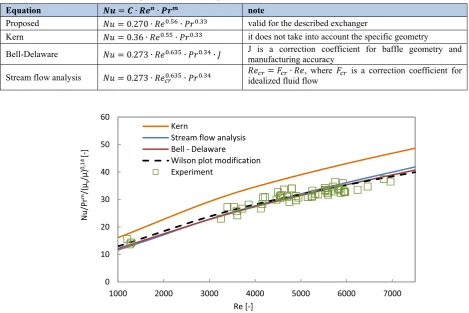
The proposed criterion equation is compared with the most commonly used theoretical methods – the methods by Kern, Bell-Delaware and Stream flow analysis (see Table 1). These methods are described in detail in [6].

For simplicity, the term ቀఓ

ఓೞቁ

଴Ǥଵସ

is not shown in the table.

The proposed coefficients C and n reach similar values as the coefficients used in the theoretical methods. Fig. 6 shows that the proposed equation achieves good agreement with the experimental results and also with the Bell-Delaware method and Stream flow analysis. The Kern method does not take into account the heat exchanger geometry, e.g. manufacturing clearances and resulting leakages, and it gives higher values.

9 Conclusion

A modification of the Wilson plot method for shell-and-tube condensers was proposed. The modification is based on the validation of the Nusselt theory for calculation of the HTC on the condensation side. The thermal resistance on the condensation side varies depending on different conditions of the total heat transfer process and is part of the calculation. It is possible to improve the determination accuracy of the convection coefficients using the proposed modification.

For the described heat exchanger, the criterion

Fig. 6. Comparison of methods for the calculation of the HTC 0

0.5 1 1.5 2

0 0.5 1 1.5 2

h

experiment

[kW/m

2K]

h theory[kW/m2_K]

experiment theory=experiment ±8%

Table 1 Comparison of criterion equation for calculation of the Nusselt number Equation ࡺ࢛ ൌ ࡯ ή ࡾࢋ࢔_{ή ࡼ࢘}࢓ _note

Proposed ܰݑ ൌ ͲǤʹ͹Ͳ ή ܴ݁଴Ǥହ଺ή ܲݎ଴Ǥଷଷ valid for the described exchanger

Kern ܰݑ ൌ ͲǤ͵͸ ή ܴ݁଴Ǥହହή ܲݎ଴Ǥଷଷ it does not take into account the specific geometry

Bell-Delaware ܰݑ ൌ ͲǤʹ͹͵ ή ܴ݁଴Ǥ଺ଷହή ܲݎ଴Ǥଷସή ܬ J is a correction coefficient for baffle geometry and manufacturing accuracy

Stream flow analysis ܰݑ ൌ ͲǤʹ͹͵ ή ܴ݁_௖௥଴Ǥ଺ଷହή ܲݎ଴Ǥଷସ ܴ݁_{idealized fluid flow} ௖௥ൌ ܨ௖௥ή ܴ݁, where ܨ௖௥ is a correction coefficient for

0 10 20 30 40 50 60

1000 2000 3000 4000 5000 6000 7000

Nu/Pr

m/(

s

/)

0,14

[]

Re[] Kern

Streamflowanalysis BellDelaware

equation for the calculation of the Nusselt number was proposed. The theoretical results of the proposed equation were compared with the measured values. Correspondence between the theoretically and the experimentally determined values is located in the range of ± 8%. The proposed coefficients C and n reach similar values as the coefficients found in the most commonly used theoretical methods. The proposed equation achieves better agreement with the experimental results as well as good compliance with the Bell-Delaware method and Stream flow analysis. The Kern method does not take into account the heat exchanger geometry and its results have higher values take into account the heat exchanger geometry and Stream flow analysis.

The modified method for the determination of the shell-side HTC was used in the subsequent research of the conditions of steam-air mixture condensation in the tubes, where the effect of noncondesable air on the condensation process was analysed.

This work has been supported by Norway Grants 2009-2014, project ID: NF-CZ08-OV-1-003-2015 and the Grant Agency of the Czech Technical University in Prague, grant no. SGS 14/183.

Nomenclature

A heat transfer area (m2) C constant of geometry (-) c specific heat capacity (J/kgK) d diameter (m)

D characteristic diameter (m) g gravitational acceleration (m/s2) h convection coefficient (W/m2K) hfg latent heat of condensation (kJ/kg)

k thermal conductivity (W/mK) L tube length (m)

Tlog logarithmic mean temperature difference (K)

M mass flow rate (kg/s) Nu Nusselt number (-) Pr Prandtl number (-) R thermal resistance (K/W) Re Reynolds number (-) Q rate of heat transfer (W) S flow cross-section (m2) T temperature (K)

U overall heat transfer coefficient (W/m2K) v velocity (m/s)

dynamic viscosity (Pa·s) kinematic viscosity (m2/s) Subscripts

f fluid i inner in inlet l liquid o outer out outlet ov overall s wall t tube w water

References

1. J. Fernández-Seara, F. J. Uhía, J. Sieres, A. Campo, Applied Thermal Engineering 27, 2745 (2007). 2. J. Havlik, T. Dlouhy, Acta Polytechnica 55, 306

(2015).

3. P. Kracik, J. Pospisil, Acta Polytechnica 55, 329 (2015).

4. V. R. Naik, V. K. Matawala, IJEAT 2, 362 (2013). 5. F. Hewitt, G. L. Shires, T. R. Bott, Process Heat

Transfer (Begell House, New York, 2000).