A COMPARATIVE STUDY OF THE EFFECT OF ADAPTIVE SLICING WITH UNIFORM SLICING IN SLS PROCESS

1234 |

P a g e

A COMPARATIVE STUDY OF THE EFFECT OF

ADAPTIVE SLICING WITH UNIFORM SLICING IN

SLS PROCESS

S. Ajay Kumar

, P.Shashidhar

1,2_{Assistant Professor,}

Department of Mechanical Engineering

Mahatma Gandhi Institute of Technology Hyderabad, (India)

ABSTRACT

A great deal of rapid prototyping is involved in the slicing of a cad model. The slicing process has a direct effect on the length of time to build the prototype, as well as on the quality of the finished product. In general, the current manufacturing process uses traditional slicing methods which slice the model in uniform layer thickness. The user must make a choice between part accuracy (thin slices) and build speed (thick slices). Theoretically, the part built by the RP machine should be equivalent to the 3-D CAD model if layer thickness can be built thin enough. However, in reality, most commercial RP systems use uniform slicing procedures with a fixed layer thickness to build parts. Therefore a long fabrication time is necessary for the thin layer. Adaptive slicing algorithm minimizes this fabrication time. In this project, a comparative study is carried out for adaptive slicing method with uniform slicing method in SLS process is done. For these, adaptive slicing algorithm is implemented, which is based on cusp height concept. For this, a simulation package is developed using “C” language. The adaptive slicing algorithm is implemented using the cusp height concept. The simulation is done for two models i.e. both cube and sphere. The simulated results obtained using both uniform and adaptive slicing is compared by producing the same models viz. cube and sphere in FORMIGA P100 SLS machine.

I. INTRODUCTION

1235 |

P a g e

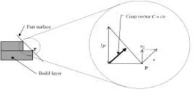
The adaptive slicing algorithm was implemented for two models based on cusp height concept. These concept was introduced by dolenca and makela[1].The layer thickness, t at a point, P is computed based on the cusp height c, within the user specified maximum allowable cusp height, Cmax as shown in the figure 1.

Figure 1. Cusp height

In addressing the stair-stepping problem, Dolenc and Mäkelä [5] focus on polyhedral models such as those described in the .STL file format. They observe that the layer thickness required to satisfy the specified surface tolerance, Cmax,, in the vicinity of a point P on the part surface is dependent upon NZ, the vertical component of

n which is the unit surface as shown in the figure 2.

Figure 2: Determining the build layer thickness from the cusp vector C, and the vertical component of the unit normal to the surface.

The thickness of the current layer is estimated using the normal‟s around the boundary of the preceding horizontal plane. The normal at any point, P, is given by

N = (Nx, Ny, Nz) (1)

And the corresponding cusp vector is given as

C = cN (2)

1236 |

P a g e

The layer thickness t is obtained using the following expression:

t= cmax

/

(5)

Otherwise t = tmin if t < tmin and t = tmax If t > tmax

In this project, using the cusp height concept adaptive slicing algorithm is implemented for two models i.e. Cube and Sphere.

II. LITERATURE REVIEW

S.H.Choi and Samavedam [2] proposes a Virtual Reality (VR) system for modeling and optimization of Rapid

Prototyping (RP) process. A mathematical model has been developed to estimate build-time of the Selective Laser Sintering Process (SLS). Pulak Mohan Pandey et.al [13] proposed slicing procedures in layered manufacturing. The present paper reviews various slicing approaches developed for tessellated as well as actual CAD models. Dolenc and Mäkelä [5] presented an approach to adaptive slicing that determined the layer thickness by using the cusp height concept. It demonstrates important advantages of adaptive slicing over the uniform slicing. Bacchewar et.al [1] discusses modeling and optimization of surface roughness in selective lasersintering process. He developed surface roughness model for SLS prototypes based on statistical design of experiments. S. K. Singhal et.al [15] presented a slicing procedure is presented in which statistical surface roughness model developed by Pandey and his group for SLS prototypes has been used as a key to slice the tessellated CAD model adaptively. The Adaptive slicing system is implemented as Graphic User Interface in MATLAB-7. The capabilities of developed adaptive slicing system have been demonstrated by case studies.

Justin T. Tyberg [16] presented this thesis demonstrates how to minimize fabrication times when implementing

adaptive layered manufacturing. Specifically, it presents a new method in which each part or individual part feature is assigned a distinct, independent build layer thickness according to its particular surface geometry. Ren C. Luoi et.al [11] presented the proposed adaptive slicing approach determines the layer thickness based on comparing the contour circumference or the center of gravity of the contour with those of the adjacent layer.

III. PROBLEM DEFINITION

1237 |

P a g e

In this project, a comparative study of the effect of adaptive slicing method with uniform slicing method in SLS process is done. For this, a simulation package is developed using “C” language. The adaptive slicing algorithm is implemented using the Cusp height concept. The simulation is done for two models i.e. both cube and sphere. Sphere is the most complexity geometry section among all other geometric sections in rapid prototyping. Because in upper and lower surfaces having more staircase effect compared to the center of sphere. Cube is the simplest geometry compared to all the geometric sections. The simulated results were obtained using both uniform and adaptive slicing is compared by producing the same models viz. cube and sphere in FORMIGA P100 SLS machine available in the Centre for Prototyping and Testing of Industrial Products (CPTIP) lab of Mechanical Engineering Department, University College of Engineering (UCE), Osmania University.

IV. PROPOSED SOLUTION METHODOLOGIES

This is the generalized procedure for making the model from the rapid prototyping machine.  Create a CAD model.

 Convert the CAD model to STL format;

 Slice the STL file into thin cross-sectional layers.  Construct the model one layer atop another.  Clean and finish the model.

4.1 BUILDING A CAD MODEL



The rapid prototyping process, in its simplest form, involves breaking up of a 3-D CAD model into

2-D slices. The slice data are then translated into a physical model.



In this project cube of 50x50 mm size and sphere of 25 mm radius is modeled in CATIA as shown

1238 |

P a g e

Figure 4.1 shows cube and sphere in CATIA software

4.2 CONVERSION OF CAD MODEL IN TO STL FORMAT

After getting Cad model, the next step is converted CAD model in to STL format by saving a CAD model in *stl format in ASCII mode.

4.3 SLICE THE STL FILE INTO THIN CROSS-SECTIONAL LAYERS:

After completing STL file from CAD file, this file sliced and imported to the RPT machine. For this slicing purpose so many kind of RPT software‟s available and in these project used Magics software.

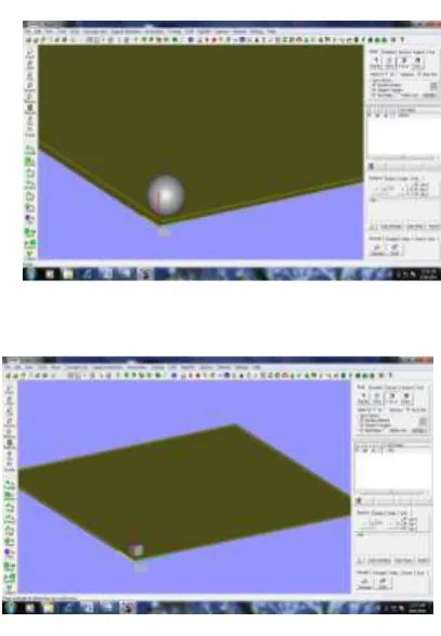
Preparing the part

The part designed must first be aligned and positioned in an RP software package, e.g. Magics RP as shown in the figure 4.2. There are some special aspects that must be taken into account for the laser sintering process. After this, the part data is transformed into layer data using the EOS RP-Tools.

1239 |

P a g e

4.4 INPUT DATA GIVEN FROM MAGICS FOR ‘C’ PROGRAM SIMULATION CODE

The STL file is taken as input for C program simulation code. As earlier describes STL file contains set vertices and normal‟s, retrieving these vertices and normal from file. Input file of cube as shown in the figure 4.3. solid CATIA STL

facet normal 2.679808e-002 7.435361e-002 -9.968718e-001 outer loop

vertex 5.197014e+001 5.402574e+001 2.012853e-001 vertex 5.204208e+001 5.373801e+001 1.817584e-001 vertex 5.170237e+001 5.311616e+001 1.262445e-001 endloop

endfacet

Figure 4.3 shows STL file in ASCII mode for cube

4.5 SIMULATION ALGORITHM

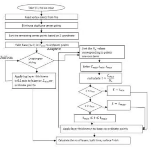
STL file of cad models consisting of set of vertex points and their corresponding normal‟s. This is the input file for c-programming and the flow chart of uniform and adaptive slicing algorithm as shown in the figure 4.4.

4.5.1 Simulation in Uniform Slicing:

The simulation procedure for both cube and sphere followed these steps. The stl files of cube and sphere were taken as inputs for this algorithm.

Step 1: Read all the lines that are started with „vertex‟. Data is read using the file read function from „fscanf‟ function. String Comparison function „strcmp‟ is used to compare the read string. When a line starting with „vertex‟ is encountered, the following data (3 float values successive) are read (X, Y, Z Co-ordinates of Cube and Sphere).

Step 2: The data is written in to a new file.

Step 3: Open the new files and read the data and write the co-ordinates into 3 arrays.

Step 4: Arrays are searched for duplicate set of co-ordinate points and duplicates are eliminated. Step 5: Read the left out co-ordinate points into another set of array.

Step 6: Start the arrays in ascending order based on Z co-ordinate.

1240 |

P a g e

Fig 4.4 Flow chart of slicing algorithm in SLS process

4.5.2 Simulation in Adaptive Slicing

STL file of cad models consisting of set of vertex points and their corresponding normal‟s. This is the input file for c-programming and gets the output of no of layers, build time and surface roughness. The corresponding simulation code for cube in APPENDIX 3. The corresponding simulation code for sphere in APPENDIX 4. The simulation procedure for cube and sphere consisting of the following steps.

 Read all the line from files that starts with “vertex”. The data is read using file read function “fscanf”.

 The data is written in to a new file.

 Open the new files and read the data and write the co-ordinates into 3 arrays.

 Arrays are searched for duplicate set of co-ordinate points and duplicates are eliminated.

 Read the left out co-ordinate points into another set of array.

 Start the arrays in ascending order based on Z co-ordinate.

 Then applying the layer thickness based on the Cusp Height (C_max) by Dolenc and Makela[5].

 The layer thickness t is obtained using the following expression:

t = Cmax / NZ here NZ ≠ 0 If tmin ≤ t ≤ tmax

1241 |

P a g e

 Then no of layers, build time and the surface roughness are taken from equations

 In this project work the maximum deviation ratio Cmax is taken as. The range of layer thickness varies from 0.1 mm to 0.3 mm.

tmin = 0.1 mm tmax = 0.3 mm

NZ Values are directly taken from input file. 4.6 TRANSFER THE STL FILE TO EOS RP-TOOLS

The STL file is transferred to EOS RP-Tools. EOS RP-Tools are used for preparing CAD data in STL format or layer data in CLI format for the building process.

During this process the data are converted into layer data in the EOS SLI format with the file extension ".sli". In the next section it is described how the data are prepared for use.

The following work sequence is generally employed for the preparation of the data:

 Slice the 3D data using the Slicer module.

 Analyze and rectify data errors using the Slifix module.

 If necessary, generate skin/core using the Skin core module.

Standard parameters for the processing of the materials are saved in EOS Default Jobs. It is very important that the default job matching the material is loaded.

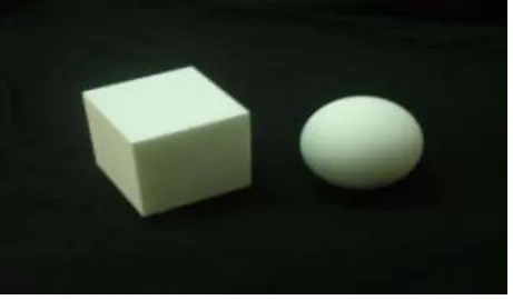
After exporting building task from PSW to SLS RP machine, the RP machine start the process to produce prototypes. The below figure 4.5 shows the Cube and Sphere from FORMIGA P100 SLS MACHINE.

1242 |

P a g e

V. RESULTS AND DISCUSSIONS

5.1 SIMULATION RESULTS IN UNIFORM SLICING BY C-PROGRAMMING:

The values obtained from simulating in uniform slicing as shown in the table 5.1. Table 5.1 Simulation Results in Uniform Slicing

component

Size

(mm)

No of

layers

Build

time

(hrs)

Surface

roughness

(µm)

Cube

50x50

500

4.86

4.68

Sphere

50 dia.

500

4.86

4.68

5.2 SIMULATION RESULTS IN ADAPTIVE SLICING BY C-PROGRAMMING:

The values obtained from simulating in simulating adaptive slicing as shown in the table 5.2.

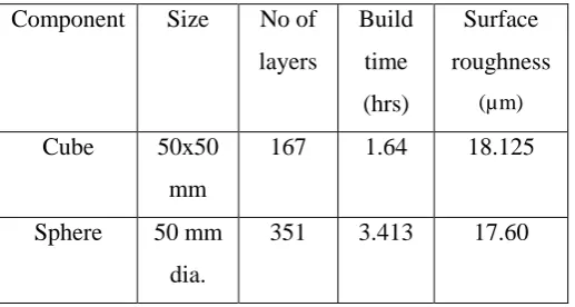
Table 5.2 simulation results in adaptive slicing

Component

Size

No of

layers

Build

time

(hrs)

Surface

roughness

(µm)

Cube

50x50

mm

167

1.64

18.125

Sphere

50 mm

dia.

351

3.413

17.60

Input data for both cube and sphere were Cmax = 0.05mm, tmin = 0.1mm , tmax = 0.3mm

, ,

1243 |

P a g e

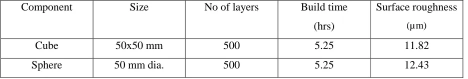
Table 5.3 SLS machine (uniform slicing) results

Component

Size

No of layers

Build time

(hrs)

Surface roughness

(µm)

Cube

50x50 mm

500

5.25

11.82

Sphere

50 mm dia.

500

5.25

12.43

The results of the uniform slicing (machine), uniform slicing (simulation) and adaptive slicing are shown in the tables 5.1, 5.2 and 5.3 respectively. Maximum relative area deviation ratio between two adjacent slices (is 0.05 units). The range of layer thickness for adaptive slicing is from 0.1 mm to 0.3 mm. The layer thickness for uniform direct slicing is 0.1 mm. For the cube and sphere, the number of layers for simulation in uniform slicing is 500 and built time 4.86 hrs, while the number of layers required for cube in adaptive slicing is reduced to 167 and built time is 1.64 hrs. For the sphere, the number of layers for simulation in uniform slicing is 500 and built time is 4.86 hrs, while the number of layers for adaptive slicing is reduced to 351 and built time is 3.413 hrs. The surface roughness values for cube and sphere in uniform slicing is 4.68µm while the adaptive slicing for cube requires 18.125µm and for sphere requires 17.60 µm.

From the FORMIGA P100SLS machine results, cube requires 500 layers, build time 5.25 hrs, the surface roughness is 11.82 µm and sphere cube requires 500 layers, build time 5.25 hrs, the surface roughness is 12.43 µm.

For comparing the simulation results of uniform slicing with SLS machine results, cube and Sphere requires built time is 5.25 hrs in FORMIGA P100 SLS machine where as the built time for cube and sphere is 4.86 hrs. It can be shown that there is slight variation between machine results with simulation results. This is due to pre heating, proper adjusting of object in the build chamber and sintering area. The below table shows the percentage reduction in build time and no of layers in adaptive slicing as compared to simulation in uniform slicing.

Table 5.4 percentage reductions in build time and no of layers in adaptive slicing compared to uniform

slicing

Components

Build time reduced (%)

No of layers reduced (%)

Cube (50x50 mm)

66.67

66.67

Sphere (50 mm dia.)

29.77

29.77

1244 |

P a g e

VI.CONCLUSIONS

In this work the comparative study of the adaptive slicing with uniform slicing process is done. The following observations were made out from the study of this project,

1. From the results it can be shown that Adaptive slicing method requires 167 layers for cube and 351 layers for sphere where as uniform slicing method requires 500 layers for cube and 500 layers for sphere. It indicates, for cube adaptive slicing was reduced 66.67% of the layers as compared to uniform slicing and for sphere adaptive slicing was reduced 29.77% of the layers as compared to uniform slicing.

2. From the results it can be shown that Adaptive slicing method requires build time 1.64 hrs for cube and 3.413 hrs for sphere where as uniform slicing method requires build time 4.86 hrs for cube and 4.86 hrs for sphere. It indicates, for cube adaptive slicing was reduced 66.67% of the build time as compared to uniform slicing and for sphere adaptive slicing was reduced 29.77% of the build time as compared to uniform slicing. 3. For both cube and sphere, this project studied the effect of surface roughness in both uniform and adaptive

slicing process. The surface roughness values for cube and sphere in uniform slicing is 4.68 µm while the adaptive slicing for cube requires 18.125 µm and for sphere requires 17.60 µm.

4. For comparing the simulation results of uniform slicing with SLS machine results it can be shown that there is slight variation between machine results with simulation results. This is due to shrinkage allowances, proper adjusting of object in the build chamber and sintering area.

Future Scope of Work:

In this project, the simulation adaptive slicing algorithm is adapted only for both cube and sphere. It can be extended to various other types of synthetic curves etc. This simulation algorithm can be extended to FORMIGA P 100 SLS machine.

REFERENCES

[1]. Bacchewar, P. B.; Singhal, S. K.; Pandey, P. M.: Statistical modelling and optimization of surface roughness in selective laser sintering process, Proc. IMechE Part B: J. of Engineering Manufacture., 221, 2007, 35-52.

[2]. S.H.Choi and Samavedam, “Modelling and Optimization Of Rapid Prototyping” computers in industry, vol 47, page no 39-53,(2002)

[3] A. Dolenc and I.Mäkelä, “Slicing procedures for layered manufacturing techniques,” Computer-Aided Design, vol. 26, no. 2, pp. 119–126, Feb, 1994.

[4]. Kamesh and Flyn, Build-time Estimator for Stereolithography Machines- A preliminary Report, Prototype Express.