A new method for the beta function in the chiral symmetry
bro-ken phase
ZoltanFodor1,2,KieranHolland3,,JuliusKuti4,DanielNogradi5,6, andChik HimWong1 1University of Wuppertal, Department of Physics, Wuppertal D-42097, Germany
2Juelich Supercomputing Center, Forschungszentrum Juelich, Juelich D-52425, Germany 3University of the Pacific, 3601 Pacific Ave, Stockton CA 95211, USA
4University of California, San Diego, 9500 Gilman Drive, La Jolla CA 92093, USA
5Eötvös University, Institute for Theoretical Physics, MTA-ELTE Lendulet Lattice Gauge Theory Research
Group, Budapest 1117, Hungary
6Universidad Autonoma, IFT UAM/CSIC and Departamento de Fisica Teorica, 28049 Madrid, Spain
Abstract.We describe a new method to determine non-perturbatively the beta function of a gauge theory using lattice simulations in the p-regime of the theory. This complements alternative measurements of the beta function working directly at zero fermion mass and bridges the gap between the weak coupling perturbative regime and the strong coupling regime relevant to the mass spectrum of the theory. We apply this method to SU(3) gauge theory with two fermion flavors in the 2-index symmetric (sextet) representation. We find that the beta function is small but non-zero at the renormalized coupling valueg2 =6.7, consistent with our previous independent investigation using simulations directly at zero fermion mass. The model continues to be a very interesting explicit realization of the near-conformal composite Higgs paradigm which could be relevant for Beyond Standard Model phenomenology.
1 Introduction
In the search for near-conformal composite Higgs theories, non-perturbative lattice determinations of the beta function of the renormalized gauge coupling have played a crucial role. The recent
de-velopment of the gradient flow [1–4] has added a new level of precision allowing for very accurate
measurement of renormalized quantities. However lattice simulations of Beyond Standard Model
(BSM) theories with an increased number of fermion flavors, likeNf = 12, or fermion
representa-tions other than the fundamental can lead to a significant increase in computational effort compared
to simulations of QCD.
To determine if a given model is infrared conformal or not, one has to know the behavior in the chiral limit. For beta function studies, that typically leads to working directly at zero fermion mass, with a particular choice of boundary conditions. There are also complementary studies of the particle spectrum of such theories, where the fermion mass is varied to see if e.g. chiral symmetry appears to be spontaneously broken in the massless limit generating a set of Goldstone bosons, or
if a light composite scalar particle, perhaps a Higgs impostor, exists in such a model. Given the large computational resources each such study requires, a beta function measurement which can take
advantage of pre-exisiting particle spectrum type gauge ensembles would be very valuable, since(a)
it would involve negligible additional computational cost,(b)the beta function would be measured
at renormalized gauge couplings strong enough to see if chiral symmetry could be spontaneously
broken in the chiral limit, and(c)it would complement independent beta function measurements from
simulations directly at zero fermion mass. In this report we describe such a technique. We apply it in the context of near-conformal gauge theories, the method can just as well be applied to other gauge theories such as QCD.
2 Gradient flow and step-scaling in finite volume
The gradient flowdAµ/dt = DνFνµ defines the gauge fieldAµ(t) at flow time t. Perturbatively, the
action densityE=(Faµν)2/4 has an expectation value
E= 3(N
2−1)g2
128π2t2
1+c1g2+O(g4) (1)
in the MS scheme for SU(N) gauge theory where the renormalized couplinggis defined at the
renor-malization group scaleµ=1/√8t. This motivates a non-perturbative definition of the renormalized
coupling
g2(t)≡ N1
128 π2
3(N2−1)
t2E
latt, (2)
where the expectation value of the action density at flow timetis measured via lattice simulations and
the normalization factorNdepends on the choice of boundary conditions. As the action density is a
bulk quantity, the observableEcan be measured non-perturbatively very precisely.
One way to measure the beta function in finite volume is via step-scaling: in a physical volume
L4, the flow is adjusted holding c = √8t/L fixed, each choice ofc corresponding to a particular
renormalization group (RG) scheme. The RG scaleµis now in terms of the only remaining scaleL.
For a given lattice volume (L/a)4the bare gauge coupling (and hence the lattice spacing) is adjusted
such that the renormalized coupling has a chosen fixed value e.g.g2c(L/a) = 6. Keeping the lattice
spacinga fixed, a second simulation on a larger volume e.g. (sL/a)4 withs = 2 gives the discrete
stepβ(g2c)={g2c(sL/a)−g2c(L/a)}/log(s2) i.e. the response of the gauge coupling as the RG scale is
changed by a finite amount. In this contextdiscretehas nothing to do with the lattice discretization.
However the beta function will contain lattice artifacts which must be removed. To take the continuum
limit, the procedure is repeated for a sequence of lattice volumes e.g.L/a=16,18,20,24,28 on each
of whichg2c(L/a)=6 is tuned via the bare coupling and larger volumes e.g. 2L/a=32,36,40,48,56
from which the discrete step is measured and the limita/L → 0 is obtained. The final result is the
continuum finite-step beta function in finite volume. This approach, widely used in QCD, has already
been applied in the context of near-conformal gauge theories [5–11].
3 Beta function in infinite volume
The main message of this report is to describe an alternative approach. Since the gradient flow defines
a renormalized couplingg2(t) at any flow timet, one can also directly measure on the same ensemble
of gauge configurations the derivativet·dg2/dt = −µ2 ·dg2/dµ2 i.e. the usual beta function with
if a light composite scalar particle, perhaps a Higgs impostor, exists in such a model. Given the large computational resources each such study requires, a beta function measurement which can take
advantage of pre-exisiting particle spectrum type gauge ensembles would be very valuable, since(a)
it would involve negligible additional computational cost,(b)the beta function would be measured
at renormalized gauge couplings strong enough to see if chiral symmetry could be spontaneously
broken in the chiral limit, and(c)it would complement independent beta function measurements from
simulations directly at zero fermion mass. In this report we describe such a technique. We apply it in the context of near-conformal gauge theories, the method can just as well be applied to other gauge theories such as QCD.
2 Gradient flow and step-scaling in finite volume
The gradient flowdAµ/dt = DνFνµ defines the gauge fieldAµ(t) at flow time t. Perturbatively, the
action densityE=(Faµν)2/4 has an expectation value
E= 3(N
2−1)g2
128π2t2
1+c1g2+O(g4) (1)
in the MS scheme for SU(N) gauge theory where the renormalized couplinggis defined at the
renor-malization group scaleµ =1/√8t. This motivates a non-perturbative definition of the renormalized
coupling
g2(t)≡ N1
128 π2
3(N2−1)
t2E
latt, (2)
where the expectation value of the action density at flow timetis measured via lattice simulations and
the normalization factorN depends on the choice of boundary conditions. As the action density is a
bulk quantity, the observableEcan be measured non-perturbatively very precisely.
One way to measure the beta function in finite volume is via step-scaling: in a physical volume
L4, the flow is adjusted holding c = √8t/L fixed, each choice of ccorresponding to a particular
renormalization group (RG) scheme. The RG scaleµis now in terms of the only remaining scaleL.
For a given lattice volume (L/a)4the bare gauge coupling (and hence the lattice spacing) is adjusted
such that the renormalized coupling has a chosen fixed value e.g.g2c(L/a) =6. Keeping the lattice
spacinga fixed, a second simulation on a larger volume e.g. (sL/a)4 withs = 2 gives the discrete
stepβ(g2c)={g2c(sL/a)−g2c(L/a)}/log(s2) i.e. the response of the gauge coupling as the RG scale is
changed by a finite amount. In this contextdiscretehas nothing to do with the lattice discretization.
However the beta function will contain lattice artifacts which must be removed. To take the continuum
limit, the procedure is repeated for a sequence of lattice volumes e.g.L/a=16,18,20,24,28 on each
of whichg2c(L/a)=6 is tuned via the bare coupling and larger volumes e.g. 2L/a=32,36,40,48,56
from which the discrete step is measured and the limita/L → 0 is obtained. The final result is the
continuum finite-step beta function in finite volume. This approach, widely used in QCD, has already
been applied in the context of near-conformal gauge theories [5–11].
3 Beta function in infinite volume
The main message of this report is to describe an alternative approach. Since the gradient flow defines
a renormalized couplingg2(t) at any flow timet, one can also directly measure on the same ensemble
of gauge configurations the derivativet·dg2/dt = −µ2 ·dg2/dµ2 i.e. the usual beta function with
an infinitesimal change in the RG scale at any particular g2 value. Note that asymptotic freedom
corresponds tot·dg2/dt>0. In comparison to the approach at fixedcin Section2, the flow timetis
not held fixed relative to the lattice sizeL/ain the new method as described in what follows. From a
sequence of ensembles with various lattice volumes, fermion masses and lattice spacings, a sequence of limits can be taken to reach the continuum infinitesimal-step beta function in infinite volume in the chiral limit.
We have previously generated a large set of such ensembles in our study of the particle spectrum of two flavor sextet SU(3) gauge theory. We use staggered fermions with stout link improvement and
the Symanzik gauge action in generating the gauge configurations as described in [12]. Our previous
lattice studies of the model found a set of massless Goldstone bosons in the chiral limit separated from massive vector, axial vector and baryonic states, with an emergent light scalar, as well as strong
evidence that the chiral condensate is non-zero at zero fermion mass [12–14]. These p-regime gauge
ensembles, already strongly indicative of near-conformal behavior, provide the basis for this beta function computation.
0 5 10 15 20 25
flow time t
6 6.2 6.4 6.6 6.8 7 7.2 7.4 7.6 7.8 8 g 2
SSC fixed g2 target
563 96 =3.20 m=0.0010
t0 = 5.487 0.077
fit starts at cfg number 50 target g2 = 6.7
Nreplica = 2
0 5 10 15
flow time t
0 0.5 1 1.5 2 2.5 3 3.5 -function
SSC -function for fixed g2 target
(t) = t dg2(t)/dt
563 96 =3.20 m=0.0010
= 0.753 0.019 target g2 = 6.7
Figure 1.(left) The gradient flow renormalized coupling
g2and (right) its associated beta function on a lattice volume 563×96 at a
Goldstone boson mass of
mπ·a≈0.08.
In Figure1we show the renormalized couplingg2and its corresponding derivativet·dg2/dtfor
one ensemble, a lattice volume 563×96 at the bare gauge coupling 6/g2
0 = 3.20 and fermion mass
ma=0.001, corresponding to a Goldstone boson massmπ·a≈0.08. The derivative is approximated
by{−F(t+2)+8F(t+)−8F(t−)+F(t−2)}/(12)=dF/dt+O(4). As opposed to step-scaling
where the flow timetis set by the choice ofc= √8t/L, in this method the value of the renormalized
couplingg2is chosen and the flow time where this value is reached is measured. We show the choice
g2(t0) = 6.7, which for this ensemble occurs att0/a2 = 5.487±0.077. (Note that this does not
correspond to the choice oft0 set byt2· Et0 = 0.3 in the original investigation of [1].) A larger
choice ofg2gives a larger statistical error ont0, however too small a value ofg2gives a beta function
distorted by large cutoffeffects, as seen on the right of Figure1fort<2. These and other constraints
we describe later influence which fixed value ofg2(t0) we choose to target.
30 35 40 45 50 55 60
L 0.05 0.06 0.07 0.08 0.09 0.1 M (L)
M = 3.2 m=0.0010
M (L) = M + c1 g1(M L, ) M = 0.08118 0.00018 c1= 0.0175 0.0019
2/dof= 0.06 Q= 0.81
fitted volumes: 403 80, 483 96, 563 96
30 35 40 45 50 55 60 65 70
L 1 2 3 4 5 6 7 t0 (L)
SSC flow FSS t0(L) = 3.20 m=0.0010
t0(L) = t0 + c1 g1(M L, )
t0 = 5.36 0.10 g1 fitted
c1= 2.15 0.61
M = 0.08118 (18) input
2/dof= 0.50 Q= 0.48
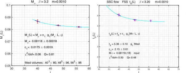
Figure 2.Infinite volume extrapolations of (left) the Goldstone boson mass and (right) the scalet0at which g2(t0)=6.7, at fixed
Since the goal is the infinite volume beta function, it is necessary to correct for finite volume
dependence. We use an ansatz with an infinite sumg1 of Bessel functions dependent on the aspect
ratio Lt/Ls of the lattice volume to account for Goldstone bosons wrapping around the finite
vol-ume [15] e.g. Mπ(L)=Mπ+cMg1(MπL) where the complicated sumg1is evaluated numerically. At
1-loop in chiral perturbation theorycM =Mπ2/(64π2F2π), we leave the prefactorcMof theg1function
as a free parameter to be fitted. In Figures2and3we show examples of such infinite volume
extrapo-lations for the Goldstone boson mass, the scalet0and the corresponding beta function. These figures
are typical: the volume effect is relatively small but visible and is well described by the ansatz. Note
that the infinite volume massMπ is first determined by the Goldstone boson volume fit and is then
used as one of the inputs for thet0and beta function volume fits.
30 35 40 45 50 55 60 65 70
L 0
0.5 1 1.5 2 2.5 3 3.5 4 4.5 5
(L)
SSC flow FSS beta function = 3.20 m=0.0010
(t) = t dg2(t)/dt
(L) = + c1 g1(M L, ) = 0.774 0.017 c1= -0.356 0.084
M = 0.08118 (18) input
2/dof= 0.24 Q= 0.63
0 0.005 0.01 0.015 0.02 0.025 0.03
m2 2
2.5 3 3.5 4 4.5 5 5.5 6 6.5 7
t0
(m
2)
t0(m2) linear chiral fit g2 = 6.7 =3.20
t0(m ) = t0(0) + c1 m2
t0(0) = 6.25 0.14
c1 = -139 14
2/dof= 0.0889 Q= 0.77
Figure 3.(left) Infinite volume extrapolation of the beta function at the renormalized coupling
g2(t0)=6.7. (right) Chiral
extrapolation of the scalet0
as a function ofM2 π. The
cyan data points are not included in the fit.
The next natural step is the extrapolation to zero fermion mass at fixed bare coupling. From [16]
if the smearing radius √8tis small compared to the Goldstone boson Compton wavelength, a chiral
expansion gives
t0=t0,ch
1+k1 M
2 π
(4πf)2 +k2
M4 π
(4πf)4log
M2 π µ2
+k3 M
4 π
(4πf)4
(3)
where f is the Goldstone boson decay constant in the chiral limit. We show in Figure3an example
of such a chiral fit of the infinite-volumet0data. We do not have sufficient data at all lattice spacings
for a quadratic fit inM2
π or to fit the chiral logarithm, hence we use a linear fit inM2π for the data at
the lighter masses. At this leading order, linear dependence inM2
π is equivalent to linear dependence
in the fermion massmitself, extrapolating in either variable to the chiral limit should give consistent
results. We show in Figure4the results of linear fits in the massmat the same bare coupling, which
are indeed consistent with extrapolating in M2
π. The determination of the scale in the chiral limit
ist0/a2 =6.20±0.14 at this bare coupling 6/g20 = 3.20, which corresponds to our coarsest lattice
spacing.
The entire procedure is repeated for two other sets of ensembles: 6/g20 =3.25 corresponding to
our intermediate lattice spacing, and 6/g20=3.30, our finest lattice spacing. We hold the renormalized
couplingg2(t0) = 6.7 fixed, find the corresponding t0/a2 and beta function values for a variety of
lattice volumes and fermion masses, fit their finite-volume dependence at fixed mass and then
extrap-olate to the chiral limit. The final step is shown in Figures5 and 6. We see that estimates of the
chiral limit scalet0/a2are 10.48±0.23 and 15.85±0.46 for the intermediate and fine lattice spacings
respectively, giving an overall change of≈ 1.6 in lattice spacing from coarsest to finest ensembles.
The chiral limit of the beta function shows modest cutoffeffects on the order of 10%, which makes
the continuum extrapolation mild. Note that a larger choice of the renormalized coupling to define the
scale e.g.g2(t0)=8 would give a larger value oft0/a2, which might not be possible to accommodate
Since the goal is the infinite volume beta function, it is necessary to correct for finite volume
dependence. We use an ansatz with an infinite sumg1 of Bessel functions dependent on the aspect
ratio Lt/Ls of the lattice volume to account for Goldstone bosons wrapping around the finite
vol-ume [15] e.g. Mπ(L)=Mπ+cMg1(MπL) where the complicated sumg1is evaluated numerically. At
1-loop in chiral perturbation theorycM=Mπ2/(64π2Fπ2), we leave the prefactorcMof theg1function
as a free parameter to be fitted. In Figures2and3we show examples of such infinite volume
extrapo-lations for the Goldstone boson mass, the scalet0and the corresponding beta function. These figures
are typical: the volume effect is relatively small but visible and is well described by the ansatz. Note
that the infinite volume massMπ is first determined by the Goldstone boson volume fit and is then
used as one of the inputs for thet0and beta function volume fits.
30 35 40 45 50 55 60 65 70
L 0 0.5 1 1.5 2 2.5 3 3.5 4 4.5 5 (L)
SSC flow FSS beta function = 3.20 m=0.0010
(t) = t dg2(t)/dt
(L) = + c1 g1(M L, ) = 0.774 0.017 c1= -0.356 0.084
M = 0.08118 (18) input
2/dof= 0.24 Q= 0.63
0 0.005 0.01 0.015 0.02 0.025 0.03
m2 2 2.5 3 3.5 4 4.5 5 5.5 6 6.5 7 t0 (m 2)
t0(m2) linear chiral fit g2 = 6.7 =3.20
t0(m ) = t0(0) + c1 m2
t0(0) = 6.25 0.14
c1 = -139 14
2/dof= 0.0889 Q= 0.77
Figure 3.(left) Infinite volume extrapolation of the beta function at the renormalized coupling
g2(t0)=6.7. (right) Chiral
extrapolation of the scalet0
as a function ofM2 π. The
cyan data points are not included in the fit.
The next natural step is the extrapolation to zero fermion mass at fixed bare coupling. From [16]
if the smearing radius √8tis small compared to the Goldstone boson Compton wavelength, a chiral
expansion gives
t0=t0,ch
1+k1 M
2 π
(4πf)2 +k2
M4 π
(4πf)4log
M2 π µ2
+k3 M
4 π
(4πf)4
(3)
where f is the Goldstone boson decay constant in the chiral limit. We show in Figure3an example
of such a chiral fit of the infinite-volumet0data. We do not have sufficient data at all lattice spacings
for a quadratic fit inM2
π or to fit the chiral logarithm, hence we use a linear fit inM2π for the data at
the lighter masses. At this leading order, linear dependence inM2
π is equivalent to linear dependence
in the fermion massmitself, extrapolating in either variable to the chiral limit should give consistent
results. We show in Figure4the results of linear fits in the massmat the same bare coupling, which
are indeed consistent with extrapolating in M2
π. The determination of the scale in the chiral limit
ist0/a2 =6.20±0.14 at this bare coupling 6/g20 = 3.20, which corresponds to our coarsest lattice
spacing.
The entire procedure is repeated for two other sets of ensembles: 6/g20 =3.25 corresponding to
our intermediate lattice spacing, and 6/g20=3.30, our finest lattice spacing. We hold the renormalized
couplingg2(t0) = 6.7 fixed, find the corresponding t0/a2 and beta function values for a variety of
lattice volumes and fermion masses, fit their finite-volume dependence at fixed mass and then
extrap-olate to the chiral limit. The final step is shown in Figures5 and 6. We see that estimates of the
chiral limit scalet0/a2are 10.48±0.23 and 15.85±0.46 for the intermediate and fine lattice spacings
respectively, giving an overall change of≈ 1.6 in lattice spacing from coarsest to finest ensembles.
The chiral limit of the beta function shows modest cutoffeffects on the order of 10%, which makes
the continuum extrapolation mild. Note that a larger choice of the renormalized coupling to define the
scale e.g.g2(t0)=8 would give a larger value oft0/a2, which might not be possible to accommodate
at the finest lattice spacing such that the finite-volume dependence could be removed. On the other
0 0.5 1 1.5 2 2.5 3 3.5 4 4.5
fermion mass m 10-3
2 2.5 3 3.5 4 4.5 5 5.5 6 6.5 7 t0 (m)
t0(m) linear chiral fit target g2 = 6.7 =3.20
t0(m) = t0(0) + c1 m
t0(0) = 6.20 0.14 c1 = -857 87
2/dof = 0.06 Q = 0.81
0 0.5 1 1.5 2 2.5 3 3.5 4 4.5
fermion mass m 10-3
0.5 0.6 0.7 0.8 0.9 1 1.1 1.2 (m)
SSC (m) linear chiral fit g2 = 6.7 =3.20
(m) = (0) + c1 m
(0) = 0.614 0.032 c1 = 164 21
2/dof = 0.075 Q= 0.78
Figure 4.Chiral extrapolations of (left) the scalet0and (right) the beta function in the fermion massm.
hand too small a value ofg2(t0) would give much larger lattice artifacts, hence the choiceg2(t0)=6.7
balances these two considerations.
0 0.5 1 1.5 2 2.5 3 3.5 4 4.5
fermion mass m 10-3
4 5 6 7 8 9 10 11 12 t0 (m)
t0(m) linear chiral fit target g2 = 6.7 =3.25
t0(m) = t0(0) + c1 m
t0(0) = 10.482 0.23 c1 = -1.76e+03 146
2/dof= 0.31 Q= 0.58
0 0.5 1 1.5 2 2.5 3 3.5 4 4.5
fermion mass m 10-3
0.4 0.5 0.6 0.7 0.8 0.9 1 1.1 1.2 (m)
SSC (m) linear chiral fit g2 = 6.7 =3.25
(m) = (0) + c1 m
(0) = 0.563 0.019 c1 = 156 11
2/dof = 0.12 Q= 0.72
Figure 5.Similar to Figure4, chiral extrapolations at 6/g20=3.25, our intermediate lattice spacing.
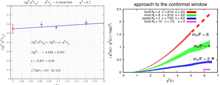
We show the last step, the continuum extrapolation of the beta function, in Figure7. In the chiral
limit we expect the leading cutoffeffect to beO(a2), hence we fit the data linearly ina2/t0, with only
three data points a more extended fitting form is not possible. Because the fitting variablet0 has its
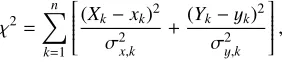
own error, this effect in included in the fit as described in [17], with theχ2function being generalized
to include the error in bothxandycoordinates
χ2=
n
k=1
(Xk−xk) 2
σ2x,k +
(Yk−yk)2
σ2y,k
, (4)
wherexk andyk are the data pairs with their respective errorsσx,k andσy,k, and Yk =c·Xk+dis
the fitting form withcanddas the parameters to be determined. Using this form, our result for the
infinite-volume infinitesimal beta function atg2=6.7 isβ(g2)=0.548±0.047. Any physical target,
noted in [18]. An alternative to the approach presented here would take the chiral and continuum
limits simultaneously in terms of √t0·manda2/t0, similar to [13]. This method is being investigated
for the beta function.
0 0.5 1 1.5 2 2.5 3 3.5 4 4.5
fermion mass m 10-3
0 2 4 6 8 10 12 14 16 18
t0
(m)
t0(m) linear chiral fit target g2 = 6.7 =3.30
t
0(m ) = t0(0) + c1 m
t
0(0) = 15.85 0.46
c
1 = -2.74e+03 396
2/dof= 0.104 Q= 0.75
0 0.5 1 1.5 2 2.5 3 3.5 4 4.5
fermion mass m 10-3
0 0.2 0.4 0.6 0.8 1 1.2
(m)
SSC (m) linear chiral fit g2 = 6.7 =3.30
(m) = (0) + c1 m (0) = 0.594 0.034 c1 = 168 31
2/dof = 0.055 Q= 0.81
Figure 6.Similar to Figures4and5, chiral extrapolations at 6/g2
0=3.30, our finest lattice spacing.
4 Comparison and conclusion
The infinite volume beta function we determine is in a different scheme than the finite volume beta
function measured via step-scaling, which in turn has its own dependence on the choice ofc, the ratio
of flow time to lattice volume. It is still instructive to compare these different results for the sextet
model as shown in Figure7, where the finite volume beta function is taken from our own work in [19].
We see that the two calculations are in good agreement – the beta function is small but non-zero in the range of renormalized couplings which, from our independent studies of the particle spectrum, are strong enough that chiral symmetry is spontaneously broken in the chiral limit. Our recent ex-tended study of the beta function of the twelve-flavor SU(3) model with fundamental representation
fermions [20] shows that at small values ofcthere is little volume dependence in the method of
Sec-tion2. This may explain the good agreement between our infinite and finite volume beta functions at
g2=6.7 in the sextet model since the new beta function in some sense might be viewed as thec→0
limit.
The finite volume beta function, calculated directly at zero mass, starts in the perturbative regime and moves to stronger coupling as the physical volume grows. If no infrared fixed point (IRFP) is found i.e. a non-trivial zero of the beta function, one could argue it is simply because strong enough coupling and large enough physical volumes have not yet been reached. However, the gauge
ensem-bles where the finite volume beta function atg2 = 6.7 could be attained are matched by p-regime
gauge configurations at the same coupling for the targeted scale but with massless fermions in the infinite volume limit and spontaneous chiral symmetry breaking. This is demonstrated by the particle
spectrum and the eigenvalues of the Dirac operator. In this phase the theory has sufficiently strong
noted in [18]. An alternative to the approach presented here would take the chiral and continuum limits simultaneously in terms of √t0·manda2/t0, similar to [13]. This method is being investigated
for the beta function.
0 0.5 1 1.5 2 2.5 3 3.5 4 4.5
fermion mass m 10-3 0
2 4 6 8 10 12 14 16 18
t0
(m)
t0(m) linear chiral fit target g2 = 6.7 =3.30
t
0(m ) = t0(0) + c1 m
t
0(0) = 15.85 0.46
c
1 = -2.74e+03 396
2/dof= 0.104 Q= 0.75
0 0.5 1 1.5 2 2.5 3 3.5 4 4.5
fermion mass m 10-3 0
0.2 0.4 0.6 0.8 1 1.2
(m)
SSC (m) linear chiral fit g2 = 6.7 =3.30
(m) = (0) + c1 m
(0) = 0.594 0.034
c1 = 168 31
2/dof = 0.055 Q= 0.81
Figure 6.Similar to Figures4and5, chiral extrapolations at 6/g2
0=3.30, our finest lattice spacing.
4 Comparison and conclusion
The infinite volume beta function we determine is in a different scheme than the finite volume beta
function measured via step-scaling, which in turn has its own dependence on the choice ofc, the ratio of flow time to lattice volume. It is still instructive to compare these different results for the sextet
model as shown in Figure7, where the finite volume beta function is taken from our own work in [19]. We see that the two calculations are in good agreement – the beta function is small but non-zero in the range of renormalized couplings which, from our independent studies of the particle spectrum, are strong enough that chiral symmetry is spontaneously broken in the chiral limit. Our recent ex-tended study of the beta function of the twelve-flavor SU(3) model with fundamental representation fermions [20] shows that at small values ofcthere is little volume dependence in the method of Sec-tion2. This may explain the good agreement between our infinite and finite volume beta functions at g2=6.7 in the sextet model since the new beta function in some sense might be viewed as thec→0 limit.
The finite volume beta function, calculated directly at zero mass, starts in the perturbative regime and moves to stronger coupling as the physical volume grows. If no infrared fixed point (IRFP) is found i.e. a non-trivial zero of the beta function, one could argue it is simply because strong enough coupling and large enough physical volumes have not yet been reached. However, the gauge ensem-bles where the finite volume beta function atg2 = 6.7 could be attained are matched by p-regime gauge configurations at the same coupling for the targeted scale but with massless fermions in the infinite volume limit and spontaneous chiral symmetry breaking. This is demonstrated by the particle spectrum and the eigenvalues of the Dirac operator. In this phase the theory has sufficiently strong
coupling to generate a p-regime with massive states separated from the massless Goldstone bosons, there is no room left at stronger coupling for the theory to have a conformal spectrum of massless states whose mass deformation would be governed by a universal anomalous dimension. This bridges the gap between the weak and strong coupling regimes and obviates any need to continue exploring even stronger coupling with the finite volume beta function in the hunt for an IRFP.
0 0.02 0.04 0.06 0.08 0.1 0.12 0.14 0.16 0.18 0.2
a2/t 0
0 0.1 0.2 0.3 0.4 0.5 0.6 0.7 0.8
(g
2,a 2/t
0
)
(g2,a2/t 0) a
2/t
0 0 chiral limit g 2 = 6.7
(g2,a2/t 0) = (g
2) + c a2/t 0
(g2) = 0.548 0.047
c = 0.321 0.44
2/dof = 1.61 Q= 0.2
0 0.5 1 1.5 2 2.5
0 1 2 3 4 5 6 7
( g
2(sL) - g 2(L) ) / log(s 2)
g2(L)
fund Nf = 4 c = 3/10 s = 3/2
fund Nf = 8 c = 3/10 s = 3/2
sextet Nfund Nf = 2 c = 7/20 s = 3/2 f = 12 c = 1/5 s = 2
approach to the conformal window
mσ/F ~ 6
mσ/F ~ 4
mσ/F ~ 2
Figure 7.(left) Continuum extrapolation of the beta function atg2(t0)=6.7, yieldingβ=0.548±0.047 as the
continuum result. (right) Comparison of this calculation with previous finite volume beta function measurements.
In the gradient flow scheme in infinite volume, the 3-loop beta function [21] has an infrared fixed point atg2≈6.8,
in the MS scheme the corresponding 3-loop beta function has a zero atg2≈6.3.
Our beta function calculations, consistent with one another, contradict other lattice studies of the finite volume beta function for the sextet model [22,23]. We believe this is because of lattice artifacts whose effects were not fully removed in those works. The range of lattice volumes we employ is
larger than in either of those studies, which allows us to push further towards the continuum. This is mostly an issue of systematic errors, not a question of underestimated statistical errors, and should be accounted for without any speculation about differing universality classes for different fermion
dis-cretizations, contrary to the claims made in [24]. Our beta function determinations are also consistent with our large-volume non-perturbative study of the particle spectrum, which shows that chiral sym-metry is spontaneously broken in the massless fermion limit, with associated Goldstone bosons and a spectrum of massive states [12–14]. This is inconsistent with other studies of the sextet model using Wilson fermion discretization, which interpret the sextet model as being infrared conformal [25].
In comparison to SU(3) gauge theory withNf massless fermion flavors in the fundamental
repre-sentation, the sextet model appears to have near-conformal behavior, with a lighter composite scalar than in theNf =4 and 8 theories. Our first investigations of the anomalous mass dimension, measured
via the Dirac operator eigenvalues, indicates that it could be sufficiently large to be
phenomenologi-cally viable [26]. If this first sign holds, and is combined with the other properties of the sextet model, the theory continues to be a relevant and interesting candidate for explicit realization of the composite Higgs paradigm. However the entangled dynamics of the light scalar and the light Goldstone pion with need for a generalized framework in chiral perturbation theory remains an unsolved problem. This is under active investigation as addressed in [27] with potential implications for the beta function analysis presented here.
Acknowledgments
Super-computing Center on Juqueen and by the Institute for Theoretical Physics, Eotvos University. We are
grateful to Szabolcs Borsanyi for his code development for the BG/Q platform. We are also grateful
to Sandor Katz and Kalman Szabo for their CUDA code development.
References
[1] M. Lüscher, JHEP08, 071 (2010), [Erratum: JHEP03,092(2014)],1006.4518
[2] R. Narayanan, H. Neuberger, JHEP03, 064 (2006),hep-th/0601210
[3] R. Lohmayer, H. Neuberger, PoSLATTICE2011, 249 (2011),1110.3522
[4] M. Luscher, P. Weisz, JHEP02, 051 (2011),1101.0963
[5] Z. Fodor, K. Holland, J. Kuti, D. Nogradi, C.H. Wong, JHEP11, 007 (2012),1208.1051
[6] A. Hasenfratz, D. Schaich, A. Veernala, JHEP06, 143 (2015),1410.5886
[7] Z. Fodor, K. Holland, J. Kuti, S. Mondal, D. Nogradi, C.H. Wong, JHEP 06, 019 (2015),
1503.01132
[8] C.J.D. Lin, K. Ogawa, A. Ramos, JHEP12, 103 (2015),1510.05755
[9] T. Appelquist, G.T. Fleming, E.T. Neil, Phys. Rev.D79, 076010 (2009),0901.3766
[10] A.J. Hietanen, K. Rummukainen, K. Tuominen, Phys. Rev.D80, 094504 (2009),0904.0864
[11] M. Hayakawa, K.I. Ishikawa, S. Takeda, N. Yamada, Phys. Rev. D88, 094504 (2013),
1307.6997
[12] Z. Fodor, K. Holland, J. Kuti, D. Nogradi, C. Schroeder, C.H. Wong, Phys. Lett.B718, 657
(2012),1209.0391
[13] Z. Fodor, K. Holland, J. Kuti, D. Nogradi, C.H. Wong,Spectroscopy of the BSM sextet model, in
35th International Symposium on Lattice Field Theory (Lattice2017): Granada, Spain(2017)
[14] Z. Fodor, K. Holland, J. Kuti, S. Mondal, D. Nogradi, C.H. Wong, PoSLATTICE2015, 219
(2016),1605.08750
[15] J. Gasser, H. Leutwyler, Phys. Lett.B184, 83 (1987)
[16] O. Bar, M. Golterman, Phys. Rev.D89, 034505 (2014),1312.4999
[17] M. Krystek, M. Anton, Measurement Science and Technology18, 3438 (2007)
[18] C. Bernard, Phys. Rev.D71, 094020 (2005),hep-lat/0412030
[19] Z. Fodor, K. Holland, J. Kuti, S. Mondal, D. Nogradi, C.H. Wong, JHEP09, 039 (2015),
1506.06599
[20] Z. Fodor, K. Holland, J. Kuti, D. Nogradi, C.H. Wong (2017),1710.09262
[21] R.V. Harlander, T. Neumann, JHEP06, 161 (2016),1606.03756
[22] Y. Shamir, B. Svetitsky, T. DeGrand, Phys. Rev.D78, 031502 (2008),0803.1707
[23] A. Hasenfratz, Y. Liu, C.Y.H. Huang (2015),1507.08260
[24] A. Hasenfratz, C. Rebbi, O. Witzel,Testing Fermion Universality at a Conformal Fixed Point,
in35th International Symposium on Lattice Field Theory (Lattice 2017) Granada, Spain, June 18-24, 2017(2017),1708.03385
[25] M. Hansen, V. Drach, C. Pica, Phys. Rev.D96, 034518 (2017),1705.11010
[26] Z. Fodor, K. Holland, J. Kuti, S. Mondal, D. Nogradi, C.H. Wong, PoSLATTICE2015, 310
(2016),1605.08091
[27] Z. Fodor, K. Holland, J. Kuti, D. Nogradi, C.H. Wong,Probingσ-model and dilaton signatures