for Restricted Boltzmann Machine
Lin Ning [email protected]
Computer Science Department, NCSU
Xipeng Shen [email protected]
Computer Science Department, NCSU
Abstract
This paper proposes Lean Contrastive Diver-gence (LCD), a modified Contrastive DiverDiver-gence (CD) algorithm to accelerate the training process of Restricted Boltzmann Machine (RBM) while maintaining the same training result achieved by the original CD algorithm. It efficiently recog-nizes and removes redundant computations from two aspects: one focuses on the sampling pro-cess, giving upper and lower bounds of the pos-sible conditional probability of each sampled unit; the other one focuses on the calculation of the conditional probability, reusing history results to speed up the computation. Experi-ments show that LCD could achieve significant speedups comparing to the original algorithm.
1. Introduction
As a generative model, Restricted Boltzmann Machine (RBM) has been used for extracting meaningful high-level representations (e.g., hidden features in images) from many different types of data input including labeled or unla-beled images (Hinton. et al.,2006;Ranzato et al.,2010), sequence of speech signals (Mohamed & Hinton, 2010), word observations (Dahl et al., 2012) and movie ratings (Salakhutdinov,2010). It is originally developed as Binary RBM in which both the visible and hidden layers are binary units. Variations (e.g., Gaussian-Bernoulli RBM) are intro-duced to deal with real value observations and other types of input. RBMs can also be stacked to form deep learn-ing networks like Deep Belief Network and Deep Boltz-mann Machines (Hinton. et al.,2006;Bengio et al.,2007; Salakhutdinov & Hinton,2009;Nair & Hinton,2009; Sri-vastava & Salakhutdinov,2012).
For many machine learning algorithms, the training is based on gradient descent. However, the loss function of RBM is intractable so it is difficult to use gradient descent directly. Therefore, Contrastive Divergence (CD) learning procedure (Hinton,2002;2010), an approximation to gra-dient descent, is used to train RBM. It creates a Markov Chain for each data point and runs Gibbs Sampling for sev-eral iterations to get a low variance estimation of the equi-librium states distribution under the RBM model. CD-k represents a CD algorithm with k Gibbs Sampling itera-tions for each data point. It is shown that CD-10 always performs better than CD-1 (Tieleman,2008) but consumes much more time due to more Gibbs Sampling steps. Per-sistent Contrastive Divergence (PCD) (Tieleman,2008) is introduced as a faster and simple alternative of the original CD algorithm. Other Efforts (Tieleman & Hinton,2009; Nair & Hinton,2010;Cho et al.,2011;Tang & Sutskever, 2011;Courville et al.,2011;Tran et al.,2013;Yamashita et al.,2014;Wang et al.,2014) have also been taken to find efficient and better ways to train the model.
op-timization. Section3.4shows that LCD could be applied to variations of RBM, RBM based Deep Learning Networks and other CD based training algorithms with only small modifications. We test the performance of LCD on Binary RBMs and Gaussian-Bernoulli RBMs. We also apply our optimization to PCD training algorithm (LPCD) and use it to train Binary RBMs. The experiment results are included in section4. In most of the cases, LCD achieves substantial speedups over the original CD based training algorithms.
In the rest of this paper, we first give a brief introduction of the RBM training algorithm, emphasizing the CD algo-rithm and the Gibbs Sampling process, in section 2. In section 3, we describe the optimization approaches used in LCD and its applicability to variations of RBM, Deep Neural Networks and other Training Algorithms. Section4 presents setups and results of the experiments. Finally, we summarize the work in section5.
2. RBM Training Algorithm
2.1. RBM with Binary Units
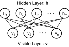
Figure 1.A Binary RBM withnvisible units andmhidden units.
hrepresents the hidden unit vector andvrepresents the visible unit vector.
As illustrated in Figure1, Binary RBM, the simplest RBM, is composed of two layers of binary units: a visible layer (v) withnvisible units and a hidden layer (h) withm hid-den units. These two layers are hid-denoted by a visible unit vectorvand a hidden unit vectorh. The state of each unit can only be 0 or 1. θ = (a,b, W)are the model parame-ters: the bias vectorsa ∈Rnandb∈Rmfor the visible
and hidden layers and the weight matrixW ∈Rn×mthat contains the weights on edges between pairwise visible-hidden units. The conditional distributions are:
P(hj= 1|v) =σ(bj+vTW(:,j)) (1)
P(vi= 1|h) =σ(ai+W(i,:)h) (2)
where σ(·) is the sigmoid activation function. Previous studies (Hinton,2010;Tieleman & Hinton,2009) showed that the updating rules forθduring the training process with
a learning rateare the following:
∆Wij =(hvihjid− hvihjim) (3)
∆ai=(hviid− hviim); ∆bj=(hhjid− hhjim) (4)
whereh·id andh·im are the expectations under the distri-bution specified by the training input data and the theoret-ical RBM model. Although computinghvihjid is
straight-forward,hvihjim is intractable due to the large number of
possible joint(v,h)configurations.
2.2. Contrastive Divergence and Gibbs Sampling Process
Contrastive Divergence (CD) algorithm (Hinton,2002) is a learning procedure being used to approximatehvihjim.
For every input, it starts a Markov Chain by assigning an input vector to the states of the visible units and performs a small number of full Gibbs Sampling steps. Resulting reconstructed visible units are used to approximate the ex-pectation of the model distribution (Hinton, 2010; Ben-gio,2009). The detailed algorithm for processing a whole dataset is shown in Alg.1.
The main part of CD is the Gibbs Sampling process. As shown in Alg.1 lines 11 - 18, a full Gibbs Sampling step includes sampling visible units given the hidden layer and then sampling the hidden units given the reconstructed vis-ible layer. Based on how many full Gibbs Sampling steps are performed, the algorithm is named as CD-k with k
standing for the number of steps.
Tieleman (2008) observed that 10 outperformed CD-1 for almost all tested cases. Although it takes longer for CD-10 to finish a same number of epochs, CD-10 always achieves a larger log-likelihood with a same time of train-ing. After a close study of CD, we find some redundant computations in the Gibbs Sampling process. By eliminat-ing those computations, there are opportunities to speed up the training algorithm. CD-k withk > 1then costs much less and is preferable due to better learning result.
3. Optimizing the CD Algorithm
The main computation of the original CD algorithm comes from the k-steps Gibbs Sampling when k>1. There-fore, optimizing this part could largely reduce the execu-tion time. We utilize two different approaches to remove redundant computations in this part.
Algorithm 1original CD algorithm
1: Input: input dataset, number of inputsN, batch size Nb, number of training epochsNe, number of gibbs sampling stepsk, input vector dimensionn, size of hid-den layerm
2: fore= 1toNedo
3: forbatch= 1toN/Nbdo
4: forq= 1toNbdo
5: Let theqthinput be vectorv d
6: forj= 1tomdo
7: P+(hj = 1|vd) =σ(bj+vTdW(:,j)) 8: hj=rand()< P+(hj = 1|vd)
9: end for
10: forstep= 1tokdo
11: fori= 1tondo
12: P(vi= 1|h) =σ(ai+W(i,:)h) 13: vi=rand()< P(vi= 1|h)
14: end for
15: forj= 1tomdo
16: P(hj = 1|v) =σ(bj+vTW(:,j)) 17: hj=rand()< P(hj= 1|v)
18: end for
19: end for
20: fori= 1tondo
21: forj= 1tomdo
22: < vihj>d= vd,i·P+(hj = 1|vd)
23: < vihj>m= vi·P(hj= 1|v) 24: ∆Wij + = (hvihjid− hvihjim) 25: ∆ai + = (hviid− hviim) 26: ∆bj + = (hhjid− hhjim)
27: end for
28: end for
29: end for
30: update parametersθ= (a,b, W) 31: end for
32: end for
in line 12 orvTW
(:,j)in line 16), which is time
consum-ing. Also, the memory access is expensive here because the Gibbs Sampling process goes though the wholeW ma-trix in order to sample a hidden or visible layer once. The main idea of Bound optimization is to give upper and lower bounds of the dot product result instead of calculating the exact value. In this way, we may be able to avoid some of the expensive dot-product computations as well as saving memory access time.
The second one, Partial Dot Production, is inspired by the fact that only a few units change their states between two consecutive Gibbs Sampling of either the visible layer or the hidden layer after training for a while. Therefore, to computeW(i,:)horvTW(:,j), we could keep track of the
changing units and update the result from the previous
it-eration by adding or subtracting the weights corresponding to the changing units.
If not mentioned otherwise, the remaining of this section uses the sampling process of hidden units as an example.
3.1. Bound Optimization
In the Gibbs Sampling Process,hj = rand()< P(hj = 1|v) is used to sample the jth hidden unit. Since there is a comparison between the conditional probability and a random number, the information we actually need for later computation is the comparison result, not the exact value of the probability. Therefore, it is possible that some of the calculations of the probability are unnecessary. A method of obtaining the comparison result without calculating the probability could then save us a lot of work.
The method we propose is using the bounds of P(hj = 1|v)as a filter to avoid some computations. Given Eq.1, since the sigmoid function is monotonically increasing and bjis a constant, the lower and upper bounds of the proba-bilityP(hj =1|v)are
lb(P(hj= 1|v))=σ(bj+lb(vTW(:,j)) (5)
ub(P(hj = 1|v)) =σ(bj+ub(vTW(:,j)) (6)
Then ifr > ub(P(hj = 1|v))orr < lb(P(hj = 1|v)), we sethj =0 orhj =1 accordingly. Only when r falls
betweenlb(P(hj =1|v))andub(P(hj =1|v)), we
com-pute the exact value of the probability using Eq.1.
To define the bounds ofvTW(:,j), we explore two different
ways in this paper: one simply adds the weights and the other makes use of the triangular inequality.
3.1.1. BOUND WITHWEIGHTSUMMATION(WS)
LetWmin+ ,j,Wmax− ,j be the minimum positive weight and the maximum negative weight inW:,j. NW+:,j andN
−
W:,j
are the number of non-negative and non-positive weights inW:,j. Nv1 is the number of units with a state of1 in
the visible unit vectorv. We use the following formulas to estimate the bounds of the dot product:
lb(vTW(:,j)) = X
i
Wij−+max(0, Nv1−NW−:,j)·W +
min,j
(7)
ub(vTW(:,j)) = X
i
Wij++max(0, Nv1−NW+
:,j)·W
− max,j
(8) Taking Eq. 7 as an example, we first add the negative weights to get a lower bound. IfN1
vis larger thanNW−:,j, it
means there are visible units with a state of 1 corresponding to positive weights. In that case, we multiply the difference betweenN1
v andN
−
to get a tighter lower bound. In a similar way, we could calculate the upper bound as shown in Eq.8.
Overhead Analysis:To get the summations of positive and negative weights in each weight vectorW:,j, the algorithm need to go through the entire weight matrix once, result-ing in a computation overhead ofO(mn). It seems to be a large overhead since it is comparable to the computation complexity of a full Gibbs Sampling step. However, the summations could be reused as long as the weight matrix doesn’t get updated. Therefore, when training RBM with the CD-k algorithm, we could reuse the calculated bounds across k Gibbs Sampling steps for processing a training in-put. Moreover, the training inputs set are usually divided into batches with a batch size ofNb(which is usually 100 or more). The weights as well as the biases are updated af-ter processing a batch of inputs. Considering this, we only need to update the summations once per batch and the com-putation overhead remainsO(mn)for processing a whole input batch.
The remaining part of bounds calculation are about finding the maximum and minimum weights inW:,j, counting the number of positive and negative weights inW:,jand count-ing the number of 1s in the visible unit vectorv. Informa-tion about the weights could be gathered while calculating the summations of positive and negative weights.N1
v could
be counted by adding a counter when sampling the visible units (lines 11-14 in Alg.1). Overall, the overhead brought by WS is negligible.
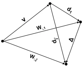
3.1.2. BOUND WITHTRIANGULARINEQUALITY(TI)
Another way to calculate the bounds ofvTW(:,j) can be
obtained by representing the vector dot product as
vTW:,j =
1 2(kvk
2
+kW:,jk
2
−d2j) (9)
with dj = kv−W:,jk. As illustrated in a 2d space in Fig. 2, given v, W:,1, W:,j0 with j0 6= 1 and ∆ =
kW:,j0−W:,1k, we have
|d1−∆| ≤dj0 ≤d1+ ∆ (10)
Combining Eq.9and Eq.10, we calculate the bounds as
lb(vTW(:,j)) = 1 2(kvk
2
+kW:,j0k2−ub(dj0)2) (11)
ub(vTW(:,j)) = 1 2(kvk
2
+kW:,j0k2−lb(dj0)2) (12)
An advantage of this method comparing to the previous one is that it could be applied directly to Gaussian-Bernoulli RBM which takes real number inputs.
Overhead Analysis: Calculating the bounds in this way introducing more overheads since we need to maintain
Figure 2.A 2d illustration of vector representations of visible vec-torv,W:,1,W:,j0,d1,dj0and∆
kW:,jk,∆andkvk. We use∆ = kW:,j0−W:,1kall the
time in order to simplify the algorithm and to reduce the overhead. The computation complexity of kW:,jk and∆ are bothO(mn). However, we only need to update them after processing a batch of inputs. If the batch size if large, this overhead is relatively small. Similarly, we only need to calculatekvkonce when sampling the hidden unit vector in one Gibbs Sampling process. Then the overheadO(n) is small compared toO(mn)whenmis large.
3.1.3. BENEFITBROUGHT BYBOUNDOPTIMIZATION
Using the sampling process of hidden units as an example, the original CD goes through the entire weight matrix in or-der to sample the whole hidden unit vector. The computa-tions required for sampling each hidden unit isO(n)where
n is the number of visible units. Therefore, the computa-tion complexity of calculating the condicomputa-tional probability in each Gibbs sampling step is O(mn)withm denoting the number of hidden units. The total computations needed for the k-steps Gibbs Sampling isO(kmn).
In the Bound optimization, we first compute the bounds. If the randomly generated number falls out of the bounded range, the computations needed to generate a sample is
O(1) without counting the overhead. Otherwise, it is
O(n), which is the same as the one needed by the origi-nal CD. The overall speedup we could achieve depends on the amount of the removed computations and the overhead introduced by calculating the bounds ofvTW
(:,j).
Let f be the fraction of hidden units sampling calcula-tions on which our bounds filter works successfully. Then the computation complexity of our optimization for pro-cessing a batch of input comes from three main parts: the bounds maintenance (O(mn)for WS based approach or O(mn+Nbkn)for TI based approach), the probabil-ity calculation when the bounds filter works successfully (O(fNbkm)for both of the approaches) and the probability
for both of the approaches). Comparing to the original CD-k algorithm which requiresO(Nbkmn)computations, our
method is more efficient than the original algorithm when
f is large.
Experiments show that the amount of computations re-moved by the TI based approach is similar to the amount achieved by the WS based approach. Since the WS based approach has a smaller overhead, we use it to calculate the bounds in all the experiments other than those with Gaussian-Bernoulli RBM. For Gaussian-Bernoulli RBM, since TI based approach could be used without modifica-tion, we implement it to calculate the bounds.
3.2. Partial Dot Production (PDP)
In either the visible layer or the hidden layer, we observed in the experiments that differences only exist in a few units between any two consecutive Gibbs Sampling steps, which means only a few units flip from 0 to 1 or from 1 to 0, after training RBM for a while. Fig.4illustrates how the fraction of flipping units changes across epochs for both the hidden layer and the visible layer with a learning rate of 0.01 on the MNIST dataset. The fraction is not very large at the beginning and drops dramatically at later epochs. We will discuss this experiment result more in section4. Based on this result, we could assume that after training the RBM for a while, a large fraction of visible units and hidden units has a high probability to stay in the same state in two succes-sive Gibbs Sampling steps for a training input under most situations.
Utilizing this feature could help us remove a lot of redun-dant computations. We still use the sampling of hidden unit vector as an example here. Letvq be the visible unit
vec-tor used to sample the hidden unit vecvec-torhq+1 during the (q+ 1)th Gibbs Sampling step. Usecjq to represent the input of the sigmoid function such that
cqj =bj+ (vq)TW(:,j) (13)
Hence the formula for calculating the conditional prob-ability of turning on the jth hidden unit becomes P(hjq+1 =1|vq) =σ(cq
j). LetS0→1 andS1→0 be the
sets of visible units which change their states (0 →1 and
1 →0) during the sampling of vq+1. For example, if
vq ={0,1,1,0}andvq+1 ={0,0,1,1}, we construct the sets asS0→1 ={v4}andS1→0 ={v2}. In the(q+ 2)th
Gibbs Sampling step, when calculating the probability us-ingP(hjq+2 =1|vq+1) =σ(cq+1
j ), instead of computing
cqj+1 =bj+ (vq+1)TW
(:,j), we calculate
cqj+1=cqj+ X
vt∈S0→1
vqt+1wtj− X
vt∈S1→0
wtj (14)
In this way, we reuse the result computed from the pre-vious iteration and only calculate the partial dot
prod-uct P
vt∈S0→1v
q+1
t wtj instead of the full dot product
P
iv q+1
i wij. This optimization could speed up both the training and the predicting processes.
Benefit and Overhead Analysis: The overhead of PDP mainly comes from the maintain of the two setsS0→1 and S1→0, which isO(n)for sampling the hidden unit vector.
Letfv be the fraction of flipping units in the visible unit vector. The computation complexity of using PDP for a Gibbs Sampling step isO(2fvmn). Whenfvis small, PDP could bring significant speedup over the original CD.
3.3. Combing the Two Approaches
We observe that the Bound optimization works better at the beginning of the training while PDP works well in the later stage. Therefore, it could be a good idea to combine these two approaches together to achieve an even better perfor-mance for the whole training process.
There are two major factors affect the design of the com-bined version. First, PDP may be able to remove a lot of computations when the Bound optimization fails in the early stage of training. Second, if we apply the Bound op-timization for every unit and change to PDP if the bounds filter fails, the choice of the current iteration will affect the computations needed in the next iteration if PDP is cho-sen in the next iteration. As shown in Eq.14, we need to knowcjqin order to calculatecjq+1 using PDP. However, if the Bound optimization works in the current iteration, the unithj is set to 0 or 1 directly without calculating the
ex-act value ofcjq. Then in the next iteration, if the Bound optimization fails, we cannot benefit from PDP because we don’t knowcqj.
Taking these two factors into consideration, we design the Combined version in a way such that each of them has a chance to be chosen for each Gibbs Sampling step during the entire training process. For each Gibbs Sampling step, we compare the expected computations (hcompi) required by both of the approaches and choose the one with a small
hcompi. If choosing the Bound optimization, for the units on which the Bound optimization fails, we apply PDP ifcjq
is calculated in the previous iteration.
3.4. Application to Variations of RBM, Deep Neural Networks and Other Training Algorithms
Binary RBM is a special class of RBM. Gaussian-Bernoulli RBM and other kinds of RBMs are proposed to learn from non-binary data images or other types of input. These vari-ations of RBM could also benefit from our optimization. Taking Gaussian-Bernoulli RBM as an example, the visi-ble units are real values while the hidden units are binaries. Therefore, the Bound optimization could be used for pling the hidden units while PDP could be used for sam-pling the visible units. For deep networks such as Deep Belief Network and Deep Boltzmann Machine, the first layer could be either a binary RBM or a Gaussian-Bernoulli RBM, and the stacked following layers are binary RBMs, so our optimization could also be applied to them directly.
As mentioned in section1, some algorithms introduce ap-proximations to the original CD in order to optimizing the RBM training process. As long as these algorithms have the Gibbs Sampling process, or perform the calculation of the conditional probability of turning on a unit in the same way, our optimization could be used. For example, PCD is an approximation of the CD algorithm. Instead of starting a Markov Chain for every input, it starts a chain for every input in a batch. The total number of the Markov Chain is equal to the batch size. Then when a batch of new inputs come into the model, the Markov Chains start at the points where they stop and continue the sampling process. This method is shown to have better performance than CD-1, even CD-10 in most of the experiments (Tieleman,2008). Our optimization could be applied directly to PCD since it has no difference from CD considering the Gibbs Sampling steps.
4. Experiments
We evaluate the efficiency of our optimization on both of Binary RBM and Gaussian-Bernoulli RBM over a variety of real world datasets. For Binary RBM, we study the per-formance of LCD and LPCD over six datasets: the MNIST handwritten digits dataset (LeCun et al.,1998), the CalTech 101 Silhouettes dataset (Marlin et al.,2010), the MICRO-NORB dataset (Tieleman & Hinton,2009), the small 20-Newsgroup dataset (Marlin et al.,2010) and the UCI repos-itory Abalone dataset (Bengio et al.,2007). Experiments are also preformed on the transformed MNIST (f-MNIST) dataset in which each pixel flips its value (Cho et al.,2011). For each of the datasets, the RBM is trained using differ-ent versions of CD-k and PCD-k algorithm with differdiffer-ent k values (1, 5 and 10). For the Gaussian-Bernoulli RBM, we compare the performance of LCD over the original CD with three different k values. kvalue starts from 2. For k= 1case, our optimization cannot be used because of the real value visible units. The datasets used for this part are
MNIST, f-MNIST, Abalone, a Financial dataset (Bengio et al.,2007), face image dataset CBCL (Yamashita et al., 2014) and Olivetti face dataset (Cho et al.,2013).
The learning rates are fixed during the training process and different learning rates are studied in the experiments. The number of visible units of RBM is determined by the size of the input image. Previous studies have shown that RBM is able to achieve a good training result on these datasets. Most of the configurations (e.g., # of visible and hidden units, k) we used in our experiments are adopted from these studies. Since our optimization doesn’t change the train-ing result of the original CD and calculattrain-ing the traintrain-ing data log-likelihood is expensive, we use a fixed number of epochs as the termination criteria. To compare the opti-mized algorithm with the original one, we run both algo-rithms for the same number of epochs and compare the ex-ecution time. The size of the datasets and the configura-tions of corresponding RBM setups are shown in columns 2-8 of Table1and Table2. N is the size of the dataset. n andmare the number of visible and hidden units.lris the learning rate andkis the number of Gibbs Sampling steps.
epoch
0 20 40 60 80 100
speedup
1 1.1 1.2 1.3 1.4 1.5 1.6 1.7 1.8 1.9 2
k = 1 k = 5 k = 10
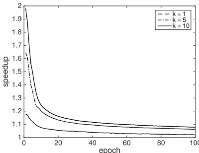
Figure 3.Speedups gained by applying the Bound optimization to the original CD-k algorithm over the MNIST dataset. The speedup is measured for every epoch and plotted as a function of epoch in this graph.
4.1. Performance of the Bound Optimization Across Epochs
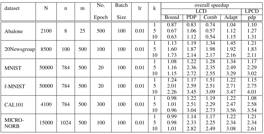
Table 1.Overall Speedups for Binary RBM with CD and PCD algorithm
dataset N n m No. Batch lr k overall speedup
LCD LPCD
Epoch Size Bound PDP Comb Adapt pdp
Abalone 2100 8 25 500 100 0.01
1 5 10 0.87 0.67 0.63 0.83 1.06 1.12 0.74 0.57 0.54 1.04 1.12 1.15 1.10 1.27 1.31
20Newsgroup 8500 100 500 100 100 0.01
1 5 10 1.13 1.60 1.73 1.19 1.87 2.14 1.34 1.98 2.17 1.45 1.92 2.16 1.21 1.83 2.11
MNIST 50000 784 500 20 100 0.01
1 5 10 1.08 1.16 1.15 1.22 2.36 2.72 1.28 2.35 2.55 1.34 2.49 3.29 1.17 2.29 3.02
f-MNIST 50000 784 500 20 100 0.01
1 5 10 1.24 2.01 2.26 1.17 2.59 3.45 1.51 2.51 3.09 1.22 2.71 3.47 1.15 2.75 4.01
CAL101 4100 784 500 300 100 0.01
1 5 10 0.98 1.01 0.96 1.22 2.51 3.04 1.19 2.29 2.73 1.22 2.47 3.56 1.08 2.58 3.54
MICRO-NORB 15000 1024 500 100 100 0.01
1 5 10 0.99 0.98 1.01 1.14 2.33 2.82 1.17 2.25 2.49 1.22 2.34 3.08 1.21 2.34 2.61
0 20 40 60 80 100
fraction of different units
0.05 0.1 0.15 0.2 0.25
k = 1 k = 5 k = 10
epoch
0 20 40 60 80 100
0 0.2 0.4 0.6 0.8
k = 1 k = 5 k = 10
Figure 4.The fraction of flipping units in both the visible and the hidden unit vectors. The upper figure corresponds to the visible unit vector while the lower figure represents the hidden unit vec-tor. The MNIST dataset is used to get these results.
at the beginning of the training. So the bounds calculated by summing the positive and negative weights are tight and able to remove many computations. However, as the model gets better trained, the weights get larger and more discrete. The summations of positive and negative weights also get larger. Due to the nature of the sigmoid function (the ”S” shape), the resulting bounds become looser quickly and the efficiency of the bounds filter decreases fast.
The results also show that a larger k value results in a larger speedup. This is because for CD, we need to compute the
epoch
0 20 40 60 80 100
speedup 1 1.5 2 2.5 3 3.5
k = 1 k = 5 k = 10
Figure 5.Speedups gained by applying the partial-dot-product optimization (PDP) to the original CD-k algorithm over the MNIST dataset. The speedup is measured for every epoch and plotted as a function of epoch.
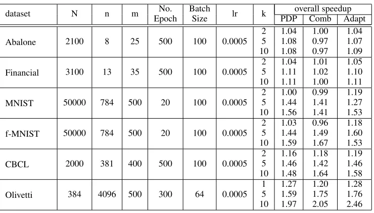
Table 2.Overall Speedups for Gaussian-Bernoulli RBM with CD algorithm
dataset N n m No. Batch lr k overall speedup
Epoch Size PDP Comb Adapt
Abalone 2100 8 25 500 100 0.0005
2 5 10
1.04 1.08 1.08
1.00 0.97 0.97
1.04 1.07 1.09
Financial 3100 13 35 500 100 0.0005
2 5 10
1.04 1.11 1.11
1.01 1.02 1.00
1.05 1.10 1.11
MNIST 50000 784 500 20 100 0.0005
2 5 10
1.00 1.44 1.56
0.99 1.41 1.41
1.19 1.27 1.53
f-MNIST 50000 784 500 20 100 0.0005
2 5 10
1.03 1.44 1.59
0.96 1.49 1.67
1.18 1.60 1.53
CBCL 2000 381 400 500 100 0.0005
2 5 10
1.16 1.46 1.48
1.18 1.42 1.64
1.19 1.46 1.58
Olivetti 384 4096 500 300 64 0.0005
1 5 10
1.27 1.59 1.97
1.20 1.75 2.05
1.28 1.76 2.46
better learning result even with a same training time. This leaves some substantial room for the Bound optimizations to take effect.
4.2. Performance of PDP Across Epochs
Figures 4 and 5 show the performance of PDP on the MNIST dataset. If a unit changes its state between two consecutive sampling steps, we call it a flipping unit. We can tell from Figure4 that the number of flipping visible and hidden units decreases during the training process, as stated in section3.2. For the visible unit vector, the frac-tion of flipping units is around 20% at the beginning of the training and drops to under 10% for all three k values. For the hidden unit vector, we mark every hidden unit from un-known to 0 or 1 in the first Gibbs Sampling step. So the fraction of flipping units of the hidden unit vector is larger than that of the visible unit vector in a same epoch. When k=1, we only sample the hidden unit vector twice. There-fore at least half of the hidden units are considered to be different from that of the previous iteration. As k increases, the first Gibbs Sampling step weights less, so the fraction of flipping units is much smaller than the k=1 case.
The speedups achieved by only applying PDP is shown in Figure5. When k=5 or k=10, the fraction of flipping units in both of the visible and the hidden unit vectors are less than20% at around epoch 100. However, the maximum speedup achieved in our experiments is not 5. This could be explained by the memory access latency. Even though the computations are removed due to identical unit values, the data may still be loaded into the cache from memory if other data in the same block are used for calculation. This could result in the speedup not proportional to the
percent-age of computation being saved when applying PDP.
4.3. Overall Speedups
The overall speedups are given in Table 1 and Table 2. The rightmost 5 columns of Table 1 report the speedups of our optimized algorithms over the original ones on bi-nary RBM with CD and PCD and a learning rate of 0.01. The performance of Bound, PDP, combined version and adaptive version are shown for LCD. For LPCD, only the speedups of adaptive version are included. According to the results, our optimization works better on dataset with a larger input vector dimension. Also, a larger k value results in a larger speedup. When k=1, the overall speedups over the original algorithm are relatively small comparing to the k=5 or 10 cases. It indicates that with only one Gibbs Sam-pling step, there are only a few opportunities existing for either the bound optimization or PDP. When k increases to 5 or 10, the improvement of performance given by bound optimization itself is limited. Meanwhile, PDP brings a significant speedup. The adaptive version always achieves a speedup of larger or comparable to the other three ver-sion (except for the k=1 case of f-MNIST). The speedups achieved with a learning rate of 0.1 and 0.001 are similar.
Overall, the experiments demonstrate that our optimiza-tions could efficiently remove a lot of redundant compu-tations and bring substantial speedups with respect to the original CD-k and PCD-k algorithms.
5. Conclusion
This work studies the training algorithm of RBM and pro-poses LCD as an accelerated CD algorithm by recognizing and removing redundant computations. Choosing adap-tively among the Bound optimization, PDP and the com-bined version, LCD efficiently cut up the RBM training time by two thirds (10 sampling steps per round) without affecting the training results. It demonstrates the promise for accelerating RBM-based deep networks.
Acknowledgement
This material is based upon work supported by DOE Early Career Award and the National Science Foundation (NSF) under Grant No. 1320796, 1525609 and CAREER Award. Any opinions, findings, and conclusions or recommenda-tions expressed in this material are those of the authors and do not necessarily reflect the views of DOE or NSF.
References
Bengio, Y. Learning Deep Architectures for AI. Now Pub-lishers Inc, 2009.
Bengio, Y., Lamblin, P., Popovici, D., and Larochelle, H. Greedy layer-wise training of deep networks. In Ad-vances in Neural Information Processing Systems 19, pp. 153–160. MIT Press, 2007.
Cho, K., Raiko, T., and Ilin, A. Enhanced gradient and adaptive learning rate for training restricted boltzmann machines. InProceedings of the 28th International Con-ference Proceedings of the 28 th International Confer-ence on Machine Learning, Bellevue, WA, USA, 2011.
Cho, K., Raiko, T., and Ilin., A. Gaussian-bernoulli deep boltzmann machine. InProceedings of the IEEE Inter-national Joint Conference on Neural Networks (IJCNN 2013), pp. 1–7, Dallas, TX, 2013.
Courville, A., Bergstra, J., and Bengio, Y. A spike and slab restricted boltzmann machine. InProceedings of the 14th International Conference on Artificial Intelligence and Statistics (AISTATS), pp. 233–241, Fort Lauderdale, FL, 2011.
Dahl, G. E., Adams, R. P., and Larochelle, H. Training re-stricted boltzmann machines on word observations. In
Proceedings of the 29 th International Conference on Machine Learning, Edinburgh, Scotland, UK, 2012.
Hinton, G. Training products of experts by minimizing contrastive divergence. Neural Comput., 14(8):1771– 1800, 2002.
Hinton, G. A practical guide to training restricted boltz-mann machines. Technical report, 2010.
Hinton., G., Osindero, S., and Teh, Y. A fast learning al-gorithm for deep belief nets. Neural Comput., 18(7): 1527–1554, July 2006.
LeCun, Y., Bottou, L., Bengio, Y., and Haffner, P. Gradient-based learning applied to document recognition. Pro-ceedings of the IEEE, 86(11):2278–2324, November 1998.
LISAlab. Restricted boltzmann machines (rbm), 2016.
Marlin, B. M., Swersky, K., Chen, B., and Freitas, N. Inductive principles for restricted boltzmann machine learning. InProceedings of the 13th International Con-ference on Artificial Intelligence and Statistics (AIS-TATS), pp. 509–516, Chia Laguna Resort, Sardinia, Italy, 2010.
Mohamed, A. and Hinton, G. Phone recognition using re-stricted boltzmann machines. InAcoustics Speech and Signal Processing (ICASSP), 2010 IEEE International Conference on, pp. 4354–4357, Dallas, TX, 2010. IEEE.
Nair, V. and Hinton, G. 3d object recognition with deep belief nets. In Bengio, Y., Schuurmans, D., Lafferty, J.D., Williams, C.K.I., and Culotta, A. (eds.),Advances in Neural Information Processing Systems 22, pp. 1339– 1347. Curran Associates, Inc., 2009.
Nair, V. and Hinton, G. Rectified linear units improve re-stricted boltzmann machines. InProceedings of the 27th International Conference on Machine Learning (ICML-10), pp. 807–814, Haifa, Israel, 2010.
Ranzato, M., Krizhevsky, A., and Hinton, G. Factored 3-way restricted boltzmann machines for modeling natural images. InProceedings of the 13th International Confer-ence on Artificial IntelligConfer-ence and Statistics (AISTATS), pp. 621–628, Chia Laguna Resort, Sardinia, Italy, 2010.
Salakhutdinov, R. Learning deep boltzmann machines us-ing adaptive mcmc. InProceedings of the 27th Interna-tional Conference on Machine Learning, pp. 943–950, Haifa, Israel, 2010. Omnipress.
Srivastava, N. and Salakhutdinov, R. Multimodal learning with deep boltzmann machines. In Pereira, F., Burges, C.J.C., Bottou, L., and Weinberger, K.Q. (eds.), Ad-vances in Neural Information Processing Systems 25, pp. 2222–2230. Curran Associates, Inc., 2012.
Tang, Y. and Sutskever, I. Data normalization in learning of restricted boltzmann machines. Technical report, De-partment of Computer Science, University of Toronto, November 2011.
Tieleman, T. Training restricted boltzmann machines using approximations to the likelihood gradient. In Proceed-ings of the 25th International Conference on Machine Learning, pp. 1064–1071, New York, NY, USA, 2008. ACM.
Tieleman, T. and Hinton, G. Using fast weights to im-prove persistent contrastive divergence. InProceedings
of the 26th Annual International Conference on Machine Learning, pp. 1033–1040, New York, NY, USA, 2009. ACM.
Tran, T., Phung, D., and Venkatesh, S. Thurstonian boltz-mann machines: Learning from multiple inequalities. In
Proceedings of the 30 th International Conference on Machine Learning, Atlanta, Georgia, USA, 2013.
Wang, S., Frostig, R., Liang, P., and Manning, C. D. Relax-ations for inference in restricted boltzmann machines. In
International Conference on Learning Representations, Banff, Canada, 2014.