FPGA IMPLEMENTATION OF A RESTRICTED BOLTZMANN MACHINE FOR HANDWRITING RECOGNITION
BY TIAN XIA
THESIS
Submitted in partial fulfillment of the requirements
for the degree of Master of Science in Electrical and Computer Engineering in the Graduate College of the
University of Illinois at Urbana-Champaign, 2015
Urbana, Illinois Adviser:
ABSTRACT
Despite the recent success of neural network in the research field, the num-ber of resulting applications for non-academic settings is very limited. One setback for its popularity is that neural networks are typically implemented as software running on a general-purpose processor. The time complexity of the software implementation is usually O(n2). As a result, neural net-works are inadequate to meet the scalability and performance requirements for commercial or industrial uses. Several research works have dealt with accelerating neural networks on Field-Programmable Gate Arrays (FPGAs), particularly for Restricted Boltzmann Machines (RBMs) — a very popular and hardware-friendly neural network model. However, when using their implementations for handwriting recognition, there are two major setbacks. First, the implementations assume that the sizes of the neural networks are symmetric, while the size of RBM model for handwriting recognition is in fact highly asymmetric. Second, these implementations cannot fit a model with a visible layer larger than 512 nodes on a single FPGA. Thus, they are highly inefficient when apply to handwriting recognition application.
In this thesis, a new framework was proposed for an RBM with asymmetric weights optimizing for handwriting recognition. The framework is tested on an Altera Stratix IV GX(EP4SGX230KF40C2) FPGA running at 100 MHz. The resources support a complete RBM model of 784 by 10 nodes. The experimental results show the computational speed of 4 billion connection-update-per-second and a up of 134 fold with I/O time and a speed-up of 161 fold without I/O time compared with an optimized MATLAB implementation running on a 2.50 GHz Intel processor. Compared with previous works, our implementation is able to achieve a much higher speed-up while maintaining comparable resources used.
ACKNOWLEDGMENTS
I am taking this opportunity to express my gratitude to everyone who sup-ported me throughout the course of my master’s study. I am thankful for their guidance and advice during the project. I am sincerely grateful to them for sharing their truthful and illuminating views on a number of issues related to my study, my research, and my thesis.
Foremost, I would like to express my deepest gratitude to my advisor, Professor Shobha Vasudevan, for her continuous support and encouragement for my graduate study and research. When I started my graduate study, I knew almost nothing about research. Prof. Vasudevan was very encouraging when I was exploring different research project. I am sincerely thankful to her for giving me this opportunity to work on this project, a project that I am truly passionate about. Her inspiring talk during the group meetings motivated all of us not only to study the topics that are directly related to our research, but also to learn a different variety of subjects to widen our knowledge. Throughout my two years of master’s study, I learned a great deal from her professionalism and dedication toward her research. Without her, this thesis would would not be possible.
I would like to particularly express my appreciation to Sai Ma for countless inspiring discussions about FPGA implementation. I sincerely thank her for listening to my problems and giving me wise suggestions and encouragement. I would also like to thank Jiayi for his patient explanation of neural networks concepts when I was first introduced to this topic. I would also like to express my heartfelt thankfulness to my wonderful colleagues, friends, and family, who supported me to overcome challenges that I faced. In the end, I would like to thank Alter University Program for donating the DE4 board that I needed for this thesis.
TABLE OF CONTENTS
CHAPTER 1 INTRODUCTION . . . 1
1.1 Artificial Neural Network . . . 1
1.2 Accelerating Neural Network . . . 6
1.3 Motivation . . . 13
1.4 Contribution . . . 15
CHAPTER 2 PRELIMINARIES . . . 18
2.1 Restricted Boltzmann Machine . . . 18
2.2 FPGA Implementation of RBM with Symmetric Weight . . . 27
CHAPTER 3 OUR IMPLEMENTATION OF RBM WITH ASYMMETRIC WEIGHT . . . 31
3.1 RBM Core . . . 32
3.2 Control Units . . . 33
3.3 Stochastic Node Selection Design . . . 37
3.4 Memory Core . . . 40
3.5 Matrix Multiplication Core . . . 42
3.6 Visible Nodes . . . 44
3.7 Hidden Nodes . . . 45
3.8 I/O Interface . . . 45
CHAPTER 4 OPTIMIZATION . . . 46
4.1 Independent Multiplier vs. Two-Multiplier Adder Mode . . . . 46
4.2 Activation Function . . . 48
CHAPTER 5 EXPERIMENTAL RESULTS . . . 52
5.1 Metrics . . . 53 5.2 Resource Utilization . . . 54 5.3 Performance Comparison . . . 54 5.4 Platform Comparison . . . 55 5.5 Scalability . . . 57 CHAPTER 6 CONCLUSION . . . 61 6.1 Conclusion . . . 61 6.2 Future Work . . . 62
CHAPTER 1
INTRODUCTION
1.1
Artificial Neural Network
Artificial Neural Networks (ANNs) are computational modeling tools that are used to solve complex various real-world problems. Inspired by biolog-ical neural networks, ANNs are massively parallel computing systems that consist of numerous adaptive yet simple processing nodes that are densely in-terconnected [1]. Although ANN is an abstraction of the biological networks of the human brain, it is not a computational model which can duplicate the operations of biological neural networks. It is only a computational struc-ture that models the known functionality of the biological neural networks for solving complicated problems. Similar to biological networks, ANNs have remarkable data processing and generalization characteristics such as mas-sive parallelism, nonlinearity, robustness, fault tolerance, learning ability, generalization ability, and the ability to handle fuzzy information [2]. These characteristics are very desirable because of the following aspects [3]. First, nonlinearity allows the model to better fit data when it is complicated. Sec-ond, noise-insensitivity can provide an accurate prediction when data uncer-tainty, measurement errors, and outliers are presented in the training sample data. Third, high parallelism in the model can lead to fast data processing since multiple data sets can be processed simultaneously. Massive parallelism can also provide failure-tolerance in the system which can still provide an ac-curate prediction when part of the system failed. Last but not least, the learning ability and the adaptivity allow the system to update its internal structure in response to environmental changes, while generalizations enable applications to learn the underlying features of the given data
ANNs are abstractions of the biological neural networks and the biological neurons are the basic building blocks of the nervous system. The operation of
neurons will be briefly explained for understanding the operation of artificial neurons and the analogy between ANNs and biological neural networks.
A neuron, as shown in Fig. 1.1, is a special biological cell that acts as a basic information processing unit for the nervous system. It is composed of a cell body and two types of out-reaching tree-shaped branches: dendrites and axons. The dendrites of one neuron is connected to then axons of other neuron. The cell body, or soma, contains information about the heredity traits, plasma, and molecular equipment used for producing the material required for the neuron to function. The dendrites receive signals form the surrounding neurons and pass them to the soma. The soma collects all the signals it receives from the dendrites of its neighboring neurons, and transmits the signals through its axons to its surrounding neurons. This basic mechanism of signal transfer establishes the fundamental step of early neurocomputing and the operation of basic building units of the ANNs.
Figure 1.1: Schematic of biological neuron
The analogy between artificial neurons and biological neurons is the con-nection between the nodes that represents the concon-nection between dendrites and axons. The connection weight represents the strength of the signal re-ceived from the dendrites and the threshold function approximates the activ-ity of soma. Figure 1.2 illustrates n biological neurons with various signals strength x with connection strength w feeding into the soma with a thresh-old of b resulting in a signal y that is transmitted to other neurons through axons, and the equivalent artificial neuron system.
Figure 1.2: Signal interaction from neurons and is analogous to signal summing in ANN
An artificial neuron is a device, often called a node, with multiple inputs and one output. It receives its inputs from other nodes or an external source, and each input has an associated weight that can be adjusted through a learning process. Each neuron has two modes of operations: learning and using. During the learning mode, neurons can be trained to fire according to its firing rule which is often modeled by an activation function. During the using mode, the neurons decide to fire using the trained connection weights and its activation function.
The learning ability is a fundamental feature of intelligence, and the abil-ity to learn automatically from given examples makes ANNs both attractive and impressive. Instead of following a set of rules specified by experts, ANNs appear to learn underlying rules from a given set of training examples. Al-though the precise definition for learning is difficult to define, the learning process of ANNs can be viewed as the process of updating the internal rep-resentation of the network in response to external stimuli so that it can be trained to efficiently perform a specific task. This is done iteratively by modifying the network architecture by adjusting the connection weights ac-cording to the input training data. The performance improves over time as the weights adjusts gradually.
1.1.1
Classification of ANNs
According to one or more relevant characteristics of ANNs, they can be classified in many different ways [3]. Generally, classification is based on the function that the ANN is designed to serve (e.g., pattern association, cluster-ing), the degree of connectivity (partial/full) of the neurons in the networks, the direction of flow of the information within the networks (recurrent and nonrecurrent), and the type of learning algorithms. The ANNs can also be classified based on the learning rule of the networks (the driving engine of the learning algorithm) and the degree of learning supervision needed for ANN training. Supervised learning involved training of ANN with the target value for each input data, and using the error between the ANN solution and the corresponding target values to adjust the weights accordingly. Unsupervised learning does not require a correct answer for the training inputs. It learns by exploring the underlying structure in the data and correlates them between various data, organizing the examples into clusters based on their similarity or dissimilarity.
As examples of classification, Lippmann [4] classified ANNs according to their degree of learning supervision needed into two categories (supervised vs. unsupervised). Simpson [5] classified ANNs according to the flow of data in the networks (feedforward vs. feedback). Maren [6] proposed a hierarchical categorization based on structure followed by dynamics, then learning. Jain and Mao [2] introduced a four-level classification based on the degree of learning supervision, the learning rule, data flow in the ANN and the learning algorithm.
1.1.2
Application of ANNs
Generally, ANNs are more robust and often can provide better performance compared to other computational tools in solving a variety of challenging problems from the following seven categories.
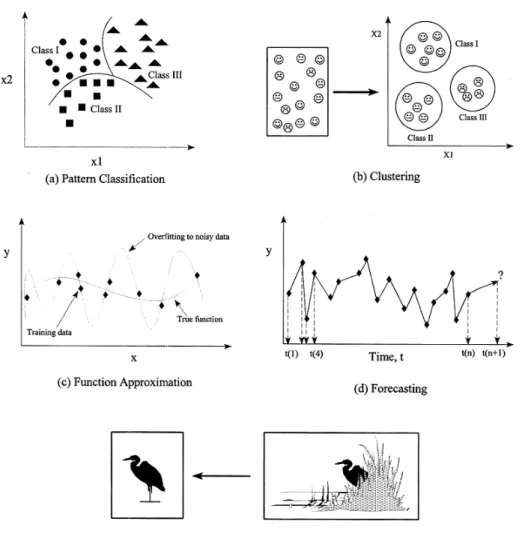
1. Pattern classification is used to assign an unknown input pattern to one of several pre-specified classes. ANNs can solve such a classification problem with supervised learning by assigning proper class labels based on one or more properties that characterized a given class, as shown in Fig. 1.3(a). Classification applications that use ANNs range from
Figure 1.3: Application of ANNs: (a) pattern classification, (b) clustering, (c) function approximation, (d) forecasting, (e) association
microbiology characteristics [7], [8], [9] to areas of computer vision and signal processing such as handwriting and speech recognition [10], [11]. 2. Unlike pattern classification, clustering is performed using unsuper-vised learning. ANNs can be trained with data with unknown class labels by exploring the similarity and dissimilarity between the neigh-boring data. The network can then assign similar patterns to the same cluster as shown in Fig. 1.3(b).
3. Function approximation includes training an ANN on input-output data so that the ANN can approximate the underlying rules or func-tions between inputs and outputs, as shown in Fig. 1.3(c). This is
extremely helpful in cases where there is no theoretical model for ob-served data available. It can also be useful when theoretical models are difficult to compute or analyze. Multilayer ANNs are considered to be the universal approximators that can approximate any arbitrary function to any degree of precision [1].
4. Prediction involves training an ANN on a set of samples representing a certain phenomenon at a given scenario at a certain time. The trained ANN is then used to predict the behavior for other scenarios at sub-sequent times. For example, as shown in Fig. 1.3(d) the ANN will be trained using data fromt(1) andt(4). The ANN is then used to predict behavior of the model form t(n) to t(n+ 1).
5. Optimization is finding the best solution to maximize or minimize an objective function subject to a set of constraints. Optimization prob-lems are a well-established field in mathematics. However, ANNs such as the Hopfield network [12] were found to be able to solve complicated and nonlinear optimization problems [13] more efficiently.
6. Association involves training a pattern associated ANN using noise-free training data. The well-trained ANN is then used to classify noisy or corrupted data. The associated neural networks should be able to reconstruct the corrupted or incomplete data. As shown in Fig. 1.3(e), the image of the bird was able to be reconstructed from the incomplete input image data. ANNs such as Hopfield and Hamming networks [4] are widely used for this application. A multilayer backpropagation ANN trained with identical input and output patterns can serve similar purposes [14].
1.2
Accelerating Neural Network
Although many existing ANN applications are usually developed as soft-ware, there are specific applications that demand high volume adaptive real-time processing, large data-set training done in reasonable real-time, and usage of energy-efficiency needed. To fulfill these requires, the ANN applications needed to be implemented in hardware since hardware can truly take
advan-tage of inherent parallelism in ANN architecture to achieve those require-ments. Hardware devices that are specifically designed to model ANN archi-tecture and associated learning algorithm can especially provide true parallel processing. These hardware devices are referred to as hardware neural net-works or HNNs. Overall, HNNs can offer the following three advantages [15].
• Speed: Specialized hardware can offer a large amount of computational power, thus it can obtain several orders of speed-up, especially in the neural network system where parallelism and distributed computing are inherently involved. For instance, very large-scale integration im-plementation for cellular neural networks can obtain speed-ups to sev-eral teraflops [16]. This speed is very high for conventional DSPs, PCs, or even workstations.
• Cost: A hardware implementation of ANN provides the possibility for reducing system cost by lowering the total number of components and decreasing the power usage. This can be extremely crucial in high-volume processing applications, such as ubiquitous consumer-products for real-time image processing, which is price-sensitive.
• Graceful degradation: A fundamental limitation of any sequential uni-processor based application is its extreme vulnerability to malfunction due to failure in the system. The primary reason for this limitation is lack of redundancy in the system architecture. As recent research indicates [17], even with modern multi-core processor architectures, the demand for effective fault-tolerant mechanisms still exits. Unlike the sequential processors, HNNs have parallel and distrusted architectures which allow the applications to continue to function while a small part of the system has failed.
1.2.1
GPUs
Recently, General Purpose Graphical Processing Units (GP-GPUs) have been identified as an intriguing technology to accelerate numerous data-parallel algorithms. ANN, on the other hand, embraces massive threads and data parallelism, which matches perfectly with GPUs. There are several attempts
to accelerate ANN training with GPUs [18], [19]. Liu and Guo [20] have pro-posed an approach which used CUDA programming model to train multilayer neural networks with back-propagation algorithm. Their implementation ex-ploits the computing power of GPUs to accelerate the training process. The experimental results have shown that their approach can achieve up to 7 times the speed-up over its CPU counterpart. Similarly, Sierra-Canto et al. [21] proposed an implementation of the back-propagation algorithm on CUDA. They used a CDUA implementation of the Basic Linear Algebra Subprograms (CUBLAS) library to simplify the training process. Their im-plementation was able to achieve 63 times faster speed than its sequential version. On the other hand, Yan Zhang and Saizheng Zhang [22] introduced an optimized deep learning architecture with flexible layer structures and fast matrix operation kernels on parallel computing platform. Their fast matrix operation kernels are implemented deep in the architecture’s propagation process which can save up to 70% of time on average compared with the kernels in CUBLAS library.
Recently, there was a study done Gu et al. [23] comparing the speed-up when using CPUs, GPUs and APUs. They implemented a multi-layer pre-ceptron and an auto-encoder on various GPUs and APUs from mainstream processor manufactures. Evaluation results have shown that GPUs are faster than APUs at the cost of burning much more power, while APUs can give better performance per watt. Around the same time, there was another study [24] done to compare performance among multi-core CPUs, GP-GPUs and Field-Programmable Gate Arrays (FPGAs) for accelerating ANN. The results have shown that FPGAs can provide highest performance but needed multiple FPGA boards to fit the entire neural network. GP-GPUs on the other hand, are able to provide flexible solution with reasonably high perfor-mance.
1.2.2
FPGAs
In FPGA implementations of ANNs, the connection weights can be stored in registers, latches, or memories. Memory storage alternatives include dy-namic RAM or static RAM [25]. Adders, subtracters, and multipliers are available on FPGAs for performing matrix multiplications. Nonlinear
acti-vation functions can be implemented using look-up tables or using adders, multipliers, etc. The FPAG implementations of ANNs entail advantages such as simplicity, low noise, flexibility and cheap fabrication [26].
Reconfigurable FPGAs provide an effective programmable hardware re-source allowing different design choices to be evaluated very quickly. The cost for modifying the design is very low and it can provide the speed of hardware and the flexibility of software. In contrast to custom VLSI, FPGAs are readily available at a reasonable price and have a reduced hardware de-velopment cycle. Moreover, FPGA-based systems can be tailored to specific ANN configuration. However, the resource density on a single FPGA is still low which limits the size of neural networks that can be implemented on a single FPGA to be thousands of neurons.
The first successful FPGA implementation [27] of artificial neural net-works was published a little over two decades ago. Since then, there have been many attempts to accelerate different ANN architectures using FPGAs [28], [29], [30], [31], [32], [33], [34], [35] for different applications ranging from speech recognition to simple classification. These proposed approaches try to optimized their design with different objectives such as speed, resource utilization, area etc. For instance, Krips et al. [36] presented an FPGA implementation of a neural network meant for designing a real-time hand detection and tracking system applied to video images. Their approaches tried to achieve reasonable processing time so that it could be useful for real-time application. Similarly, Rice et al. [37] report that a FPGA-based implementation of a neocortex inspired cognitive model can provide an aver-age throughput gain of 75 times more than the software implementation on a full Cray XD1 supercomputer. They used the hierarchical Bayesian network model based on the neocortex developed by George and Hawkins [38].
From all different FPGA implementations, there are three typical aspects that designers will try to explore with different options to optimize their designs [39].
1. Data Representation: There are multiple research works that indicate training ANNs with integer weights is possible. If weights are rep-resented as integers instead of floating points, the multipliers can be implemented more efficiently. There are a few attempts to implement ANNs with floating-points, but no successful implementation has been
reported up to the present. Nichols et al. [40] showed that despite continuing advances in FPGA technology, it is still impractical to im-plement ANNs on FPGA with weights represented with floating points. Another approach is to use a special learning logarithm [41] which uses powers-of-two integers as connection weights. The advantage of this is to simplify multipliers with series of bit shift operations.
2. Weight Precision: Selecting weight precision is one of the most impor-tant choices when implementing ANNs on FPGAs. Implementation with high weight precision will increase the implementation cost and decrease the computational speed. If weight precision is low, then it might compromise the functionality of the ANNs. The trade-off can be resolved if the minimum precision is determined. Holt and Baker [42] studied this problem by simulating using software with a set of benchmark classification problems. Their results indicate that a 16-bit fixed-point is the minimum precision without diminishing the learning ability of ANNs.
3. Transfer Function Implementation: The direct implementation of non-linear sigmoid transfer function can be very costly. There are two practical approaches to approximate the sigmoid function with FPGAs: piece-wise linear approximation or the look-up table. Piece-wise linear approximation is an approximate sigmoid function with a set of straight lines in the form of y=ax+b. If the coefficients for the lines are cho-sen to be power of 2, then the sigmoid function can be implemented using shift and add operations, which decrease the implementation cost further. The second method is to use a look-up table. The data used in the loop-up table are uniformly sampled from the sigmoid function. However, there is a trade-off with sample size and accuracy. A large sample size requires more memory which increases the implementation cost, while a small sample size leads to lower accuracy which might compromise the learning ability of the ANNs.
Besides all the detailed design choices, an important challenge that design-ers face when implementing ANN on FPGAs is to select an appropriate ANN model for a specific application so that the utilization of hardware resources can be optimal. Simon Jothson and others provide an inspiring insight on
this problem [43] by carrying out a comparative study on different ANN ar-chitectures. They implemented four different ANNs on FPGAs and analyzed the hardware requirements for each ANN structure on a benchmark classifi-cation problem. Even though their results are limited due to the number of ANN architectures they included in their study, their work provides a insight into HNNs with FPGAs.
1.2.3
Analog
Analog implementations of ANNs are usually more efficient in terms of chip area and processing speed, but this comes at the price of limited accuracy of the network component. The digital implementation, on the other hand, ensures the accuracy of the network component but with higher area cost and power consumption [44].
In analog implementations, the synaptic weights are typically stored using resistors [45], charge-coupled devices [46], capacitors [47], and floating-gate EEPROMs [48]. In VLSI, a variable resistor as a connection weight can be implemented as a circuit with two MOSFETs [49]. However, discrete values of channel length and width of the MOS transistors may cause a quantiza-tion effect in the weight value. The scalar product and subsequent nonlinear mapping are performed by a summing amplifier with saturation [50]. Un-like the digital implementation, the characteristics of the nonlinear activation function can be captured directly as a current that operates above saturation levels or as the voltage characteristics of transistors. In analog implemen-tation, signals are usually represented by currents [51] and/or voltages [49]. Current flow is preserved at each junction point by Kirchhoff current law, and during multiplication various resistance values can be used for the matrix. Thus a network of resistors can simulate the necessary network conventions and their resistances are the adaptive weight needed for learning. Overall, analog neuron implementations benefit by exploiting simple physical effects to carry out some of the network functions [52]. For instance, the accu-mulator can be a common output line to sum currents. Analog elements are usually smaller and simpler than their digital counterparts. However, obtaining a consistently precise analog circuit, especially to compensate for variations in temperate and control voltages, requires sophisticated design
and fabrication.
There has been much work done to use analog circuits to model ANNs. Ortiz and Ocasio [53] presented a discrete analog hardware model for the morphological neural networks. They replaced the classical operations of multiplication and addition with addition and maximum or minimum opera-tions. By doing so, they are able to simplify their hardware implementation. Milev and Hristov [54] presented an analog-signal synapse model using MOS-FETs to analyze the effect of the synapse’s inherent quadratic nonlinearity on learning convergence and on the optimization of vector direction. The synapse design is then used in a VLSI architecture for a finger-print feature extraction application. Similarity, Brown et al. [55] described an implemen-tation of a signal processing circuits for a continuous-time recurrent neural network using sub-threshold analog VLSI in a mixed mode approach. In their implementation, each state variable is represented as a voltage while the neural signals are represented as currents. The use of currents allows the accuracy of the signals to be maintained over long distances, which made this implementation robust and scalable.
1.2.4
Mixed Signal
Mixed signal implementations of neural networks are designed to combine the digital and analog technologies in an attempt to get the best of both. For instance, analog implementation can be used for internal processing for speed while connection weights are stored digitally. The work done by the Mesa Research Institute at University of Twente [56] used 70 analog inputs, six hidden nodes, and one analog output with 5-bit digital weights to achieve the feed-forward processing rate of 20 GCPS. The final output of the neural network had no transfer function, so that multiple chips could be added to increase the number of hidden units. Similarly, a mixed signal architecture with on-chip learning has been presented in [57]. The overall architecture is divided into two parts, analog and digital. The analog ANN unit executes the neural function processing using a charged-based circuit structure, while the units for error correction, circuit control and clock generation are kept purely digital.
1.3
Motivation
When neural networks are implemented as software running on general-purpose processors, the algorithm complexity is generallyO(n2). As a result, neural networks are unable to provide the performance and scalability re-quired in non-academic settings. There have been many attempts to design hardware implementations to speed up the performance of neural networks [58], [59]. Although a variety of approaches, from analog to VLSI systems, have been pursued, they have not resulted in widely used hardware. These attempts are typically flawed with a lack of resolution, limited neural network size, and an absence of software interfaces.
Additionally to the difficulties with the hardware implementations, another common issue is the choice of the neural network architectures. This is due to the fact that most of the neural networks are not well suited for hardware systems. For instance, one of the most common types of neural networks is the multilayer perception with back-propagation architectures [60], [61]. Although this type of neural network is very popular and used for a variety of applications, the processing elements require massive real number arithmetic as well as great deal of resource intensive components such as multipliers and accumulators. Furthermore, the transfer function for this type of neural network is also very complicated. Consequently, the hardware implementation requires a significantly greater amount of resources, which limits the scalability of the hardware. The typically solution is to introduce a pipeline to obtain parallelism. However, this approach does not result in enough parallelism and speed-up to justify the cost and effort of using such systems [28].
1.3.1
Introduction of Restricted Boltzmann Machines
A Restricted Boltzmann Machines (RBM) is a generative stochastic artificial neural network model. It is able to learn the probability distribution over a given set of inputs. It was originally invented under the name Harmoium by Paul Smolensky [62] in 1986. It did not become popular until Hinton et al. [63] introduced the fact learning algorithm for RBMs. RBMs are widely used in applications such as dimensionality reduction [64], classification [65], and feature abstractions.
In comparison with other ANN models, RBMs have hardware-friendly ar-chitectures, well suited for hardware implementation. RBMs can use data types that map well to hardware since the node states are binary-values. As a result, binary arithmetic ensures that operations can be done with simple logic gates instead of resource intensive multipliers. In some cases, the node probability is used instead of the binary-valued node state. When this hap-pens, the value for each node can only takes values from 0 to 1, and RBM does not require high precision, the node can be represented using fixed-point numbers, and the fixed-fixed-point arithmetic units can be used to decrease resource utilization and increase processing speed. The simplicity in RBM architecture allows more scalability and parallelism in hardware design.
Implementation of RBMs on FPGAs has several advantages over other hardware implementation methods for normal RBM architecture.
• One big drawback of the software implementation is that the complex-ity of the matrix multiplication needed for the learning algorithm is
O(n2). If the learning algorithm is implemented with a FPGA, the fine-grain parallelism of the FPGA can be utilized for speed up matrix multiplication.
• RBMs have a hardware-friendly structure since the data can be repre-sented using a fixed-point data type. Several previous research works have shown that only 18, or even a presentation with fewer bits is suffi-cient enough to represent the training data and the connection weights for the neural network to function correctly [66], [42], [67]. On the other hand, FPGAs have abundant embedded 18-bit by 18-bit multi-pliers available for speeding up the matrix multiplication process.
• FPGAs are rapidly growing. In addition to the raw fabric, FPGAs have various hardware components, such as on-board RAMs, DSP blocks, I/O transceivers and even processors. This allows the entire system to be implemented on the single board.
• The most important aspect of an FPGA is its ability to reconfigure. The topology of the network defines its application. The organization of processing units will define the capabilities and behavior of the neural network. Being able to implement on a reconfigurable system allows
hardware to be generated to suit the exact required topology, thus optimizing performance without sacrificing adaptability.
1.3.2
Previous Implementations of the RBMs
Recently, there have been work that introduced couple FPGA implemen-tations for training RBMs, and the handwriting recognition was used as a benchmark to compare their results with the software implementations [67], [68], [69]. The first work that tried to implement an RBM on FPAG is done by Ly and Chow [69]. They implemented a high performance RBM for general use, but their implementation did not scale well. Thus, Kim et al. [67] proposed a highly scalable implementation for RBMs. However, there are two major drawbacks in their implementations. First, all of their im-plementations are based on the assumption that connection weights have a symmetric structure and the network has the same number of visible nodes and hidden nodes. However, if their implementations are used for training the entire RBM network for handwriting recognition, their implementations would simply not work or would be highly inefficient since the visible layer is much larger than the hidden layer for a RBM trained for handwriting recog-nition application. One possible solution is to zero pad the hidden nodes to be the same size as the visible nodes. However, once the hidden layer is zero padded, the overall size of the neural network is too large for the implementations to fit the entire system on a single FPGA. Although us-ing multiple FPGAs to train one large RBM is possible [70], it is extremely inefficient when the problem can be solved using just one single FPGA. In this thesis, we proposed a new implementation called RAW, which stands for
Restricted Boltzmann machine with Asymmetric Weight. Compared with previous works, RAW is optimized for handwriting recognition and is able to perform the training process very efficiently.
1.4
Contribution
The new architecture, RAW, that we proposed in this thesis is able to train RBMs on FPGA efficiently. The implementation is also optimized for the handwriting recognition application. In RAW, we introduced a new method
to avoid the weight transpose problem. We stored each row of the weight matrix on a separate on-chip RAM, which allows the matrix multiplications to be processed in parallel. Furthermore, RAW used DSP blocks with four-multiplier adder mode to maximize the number of embedded four-multipliers avail-able for matrix multiplications. As a result, we reordered multiplication and addition operations used for the matrix. We also introduced a shift regis-ter structure to the node selection module to reduce the hardware resources needed for this implementation. As shown in Fig. 1.4, we implemented RAW on Altera Stratix IV GX that ran at 100 MHz. The results were compared with a MATLAB implementation for RBMs. The experimental results in-dicate that RAW is able to achieve a speed-up of 134 fold with I/O time and a speed-up of 160 fold without I/O time. Compared to previous works, RAW is able to achieve a much higher speed-up while the hardware resources needed are very comparable with previous works. The main reason that it is much faster is that RAW is able to calculate the matrix multiplication with more parallelism due to the structure difference in the network and imple-mentation. We also modified RAW implementation so it can be trained using different input sizes. The experimental results show that our implementation also scales well.
Figure 1.4: A picture of the Altera Stratix IV GX The rest of the thesis is organized as follows.
and two previous FPGA implementations with symmetric weights.
• Chapter 3 describes the FPGA implementation of the restricted Boltz-mann machine with asymmetric weights.
• Chapter 4 describes the optimization made for the implementation.
• Chapter 5 presents experimental results with speed-up, area, and scal-ability comparisons.
• Chapter 6 concludes the thesis with a brief discussion of possible future work.
CHAPTER 2
PRELIMINARIES
2.1
Restricted Boltzmann Machine
This section briefly discuss the terminology, mathematical background and training procedures involved in the mechanics of Restricted Boltzmann Ma-chine (RBMs). Additional details, including the historical development and statistical motivation can be found in [71], [72]. An RBM is a generative, stochastic neural network architecture. It is used to model the statistical behavior of a given set of training data.
The restricted Boltzmann machine is a generative, stochastic, and unsu-pervised learning neural network architecture. It uses statistical behaviors to model a particular set of data. Given a series of training input vectors, the network will be able to build an internal model based on the statistical distribution of the given data. Based on the training data set, the network is able to abstract the underlying properties of the input vector. The internal architecture can be used to detect whether an arbitrary data point belongs to the original input data.
The RBM is generative because the internal structure allows the network to produce new data which is consistent with the distribution. The RBM is also stochastic because it uses a probabilistic approach to model the input data. To capture statistical properties on the training data, the RBM de-termines the probability distribution of a given set with the help of random processes. These two properties, generative and stochastic, makes RMBs a unique artificial neural networks architecture.
Like all ANNs, the RBM is capable of learning. The internal structure of the RBM is mathematically defined by numerous independent parameters. Due to the state explosion of the parameter space, finding a correct set of parameters is a non-trivial task. To find the optimal parameters, the RBM
processes a set of training data, and applies the learning rules iteratively. The RBM repeatedly processes training data until it can generate desired output. Once the RBM is well trained, a new set of unexposed data, called the test data, can be used to verify its behavior.
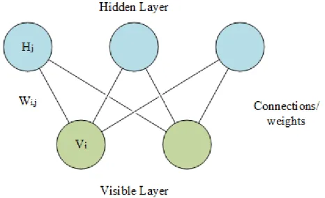
Figure 2.1: A schematic diagram of a restricted Boltzmann machine In neural networks, the processing units are often called nodes. The nodes in the RBM have binary states: on or off. As shown in the Fig. 2.1, the RBM consists of two layers of nodes, a hidden layer and a visible layer. The visible layer is used for input access while the hidden layer acts as an internal representation of the data for the networks. There are connections between every node in the two different layers, but no connections exist between nodes in the same layer. Each of these connections has an associated weight, which is the parameter that the RBM tries to optimize at each training iteration. As shown in Fig. 2.1, vi and hj are the binary states of the ith and jth nodes in the visible and hidden layers respectively. wi,j is the weight for the connection between vi and hj.
2.1.1
Alternating Gibbs Sampling
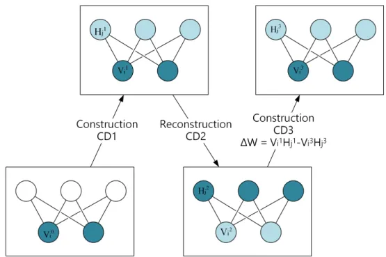
Alternating Gibbs sampling (AGS) is the training operating process for the RBM. It is the fundamental rule for generating node states and learning op-timal connection weights [73]. AGS is divided into two phases: construction
is used to determine the node state and the probability of the hidden layer. During the reconstruction phase, the hidden layer is used to generate the node state and the probability of the visible layer. The change in the weights is calculated in the last AGS phase. To begin the process, an initial data vector is loaded into the visible layer and phases are operated in an alternat-ing manner startalternat-ing with the construction phase. To differentiate the nodes between different phases, the node state will be label with the phase number as its superscript. Figure 2.2 is a representation of the AGS process.
Figure 2.2: A schematic diagram of the alternating Gibbs sampling for three phases
In order to understand how the node states are determined, the concept of global energy must be introduced first. The global energy can be simply treated as a numeric value that determines the operation and the behavior of an RBM. The global energy is defined in Eq. (2.1).
E =−X
i,j
wi,jvi, hj (2.1)
Since the weight connections only exits between nodes in different layers, the energy function can be redefined as a sum of two partial engergies. De-pending on which AGS phase is being computed, the partial energy will be calculated using different equations. The construction phase uses Eq. (2.2),
and the reconstruction phase uses Eq. (2.3). E =−X i vi( X j wi,jhj) =− X i viEi (2.2) E =−X j hj(X i wi,jvi) =− X j hjEj (2.3)
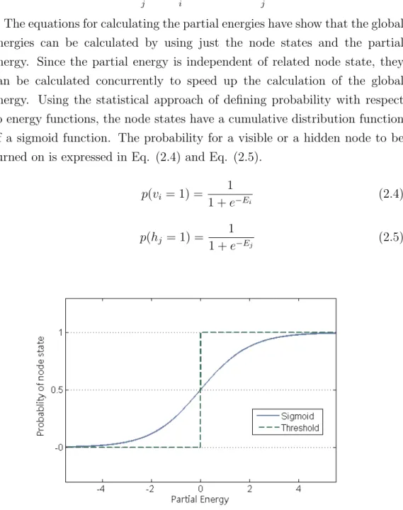
The equations for calculating the partial energies have show that the global energies can be calculated by using just the node states and the partial energy. Since the partial energy is independent of related node state, they can be calculated concurrently to speed up the calculation of the global energy. Using the statistical approach of defining probability with respect to energy functions, the node states have a cumulative distribution function of a sigmoid function. The probability for a visible or a hidden node to be turned on is expressed in Eq. (2.4) and Eq. (2.5).
p(vi = 1) = 1 1 +e−Ei (2.4) p(hj = 1) = 1 1 +e−Ej (2.5)
Figure 2.3: A plot of a sigmoid function and a threshold function To determine the node state from the sigmoid function, a uniformly
ran-dom variable must be sampled. Sometime, when the probabilistic approach is undesired, a deterministic, first-order approximation threshold function expressed in Eq. (2.6) and Eq. (2.7) is used. A comparison plot between the sigmoid function and the threshold function is shown in Fig. 2.3.
vi = ( 0, Ei <0 1, Ei ≥0 (2.6) hj = ( 0, Ej <0 1, Ej ≥0 (2.7)
2.1.2
Learning
One of the primary reasons for neural networks to be attractive is their ability to learn, and as result, the learning rules of RBMs are generating great interest [74], [75]. In the learning rules of RBMs, the connection weights are parameters used to determine the energies and node state for next AGS phase. To model a given data set, the connection weights have to be adjusted at each iteration so that the energy generated from the RBM for the entire set of training data is minimum. To find the minimum energy, the differential equation ofE with respected to the individual connection weight is expressed in Eq. (2.8). ∂E ∂wi,j =(hvihji 1 − hvihji ∞ ) (2.8)
In this equation, the h· · · iX represents the expected values of Xth AGS phase. is the learning rate of the network that is defined by the user. The node states are calculated by an iterative process of AGS. As a result, the derivative of the energy function indicates the direction vector of steepest descent in the weight space to reach the minima. Therefore, the weights must be adjusted according to the derivative at the end of every training set. This formulation raises three important points. First, the expected values of the node interactions are required over the entire set of training data to calculate the gradient descend properly. This is called batch learning. However, if the batches are large, the calculations will require a significant amount of time. One way to resolve this is to divide the batches into smaller groups. The weights will be updated with each smaller batch. This is called
mini-batch learning. If the mini-batch is still undesired, the batches can be divided into each individual input vector, and this is called on-line learning. Second, according to Eq. (2.8), the formal definition of the gradient descent requires the node state values from the infinite AGS and that is impractical to implement. Thus researchers have found that the infinite AGS phase can be replace with a small finite number. For RBMs, the lowest possible AGS phase to train the model correctly is 3.
Last, the learning rate is an independent parameter which defines the step size for each weight update. A larger learning rate leads to a faster learning process, while a smaller learning rate ensures convergence. Therefore the designers need to carefully choose the learning rate due to this trade off. Some studies suggest that the learning rate can be modified between batches to achieve a convergent solution quickly. This is called simulated annealing
[75], [74].
Although these learning algorithm shortcuts deviate from the formal def-inition of gradient descent, they enhance operational speed and are widely adapted. The learning algorithm for weight update now can be defined as shown in Eq. (2.9) and Eq. (2.10), where k is the number of batches, and L
is the number of data vectors in one batch.
wi,j[k+ 1] =wi,j[k]−(hvihji 1 − hvihji X ) (2.9) hvihji X = 1 L l X l=0 vXi hXj (2.10)
In order to make the learning algorithm easier to understand and compute, Eq. (2.1) to Eq. (2.10) can be reformulated using matrix expression. For an RBM with ivisible nodes and j hidden nodes, the visible and hidden layers can be expressed in Eq. (2.11) and Eq. (2.12) respectively.
vlX = [v0X· · ·viX−1]B1×i (2.11)
The connection weights can be reformulated as Eq. (2.13). W[k] = w0,0[k] · · · w0,j[k] .. . . .. ... wi,0 · · · wi,j[k] ∈Ri×j (2.13)
Then, the Eq. (2.1) to Eq. (2.10) can be reformulate as:
VX+1 = V0, X = 0 f(EX v ), X is odd VX, X is even (2.14) HX+1 = ( f(EX h ), X is even HX, X is odd (2.15) EvX = (HX)WT,∈Rl×i (2.16) EhX = (VX)W,∈Rl×j (2.17) W[k+ 1] =W[k] + l((V 1)TH1 + (VX)THX) (2.18) Here f(·) is the sigmoid or the threshold transfer function applied element-wise to the matrix.
2.1.3
Complexity Analysis
To understand the reason that a software implementation of the RBM run-ning on a sequential processor is not desired, the algorithm for it needs to be analyzed. The pseudo code for the software implementation of the RBM is presented in Algorithm 1. In order to make the analysis easier, we are going to assume that the RBM will have symmetric layers, where the hidden layer and visible layer have the same size (i=j =n). The algorithm for training the RBM is divided into three code block: node select, energy computation, and weight update. A detailed complexity analysis is shown in Table 2.1. As indicated in Table 2.1, the complexity of overall the algorithm is O(n2).
Algorithm 1 pseudo-code of RBM training algorithm
1: forevery batch in the training datado
2: visible []= get datavector(batch); 3: forevery AGS phasedo
4: if AGS phase is odd then
/* Engery computer Eq. (2.17) - 2 loops−→O(n2) */
5: forevery hidden nodedo
6: forevery visible nodedo
7: energy[j]+=visible[i]weight[i][j] 8: end for
9: end for
/* Node Select Eq. (2.15) - 1 loop −→O(n) */ 10: forevery hidden nodedo
11: hidden[j] = transfer function(energy[j]) 12: end for
13: else
/* Energy Compute Eq. (2.16) - 2 loop−→O(n2) */ 14: forevery visible node do
15: forvery hidden nodedo
16: energy[i] += hidden[i]*weight[i][j] 17: end for
18: end for
/* Node Select Eq. (2.14) - 1 loop −→O(n) */ 19: forevery visible node do
20: visible[i] = transfter function(energy[i]) 21: end for
22: end if
/* Weight update Eq. (2.18) - 2 loops−→O(n2) */ 23: if AGS phase == 1then
24: forevery visible node do
25: forevery hidden nodedo
26: weight update[i][j] += visible[i]*hidden[j] 27: end for
28: end for
29: else if AGS phase == AGS limitthen
30: forevery visible node do
31: forevery hidden nodedo
32: weight update[i][j]-=visible[i]*hidden[j] 33: end for 34: end for 35: end if 36: end for 37: end for
/* Weight update Using Eq. (2.18) - 2 loops−→O(n2) */ 38: forevery visible nodedo
39: forevery hidden nodedo
40: weight[i][j]+=learning rate/batch*weight update[i][j] 41: end for
Table 2.1: The complexity analysis for each code block of the RBM algorithm
Procedure Complexity Equation Node select O(n) (2.14), (2.15) Energy computer O(n2) (2.16), (2.17) Weight update O(n2) (2.18)
2.1.4
Layered Networks
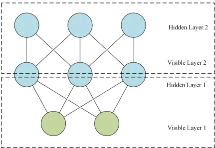
A single RBM only has one layer of visible nodes and one layer of hidden nodes. As a result, the RBM can only model first-order statistics. This limits the modeling ability of the RBM to learn when given training data with underlying properties that require higher orders of statistics for complete description. Although a single RBM has limited modeling ability, we can stack multiple RBMs together to increase its modeling ability as long as the number of nodes matches up [63]. As shown in Fig. 2.4, the hidden layer
Figure 2.4: A schematic diagram of a double-layered RBM
of one RBM will acts like the visible layer of another RBMs. The stacking is indefinite as long as there are enough resources to support the stacked RBMs. The operations and learning algorithm are changed slightly for the stacked RBMs. The individual RBMs still operate the same way, but there is a macro-algorithm to organize how the layers operate with respected to each other. More detailed description can be found in [63].
2.2
FPGA Implementation of RBM with Symmetric
Weight
Although there have been many attempts to design hardware implementa-tion of various neural network architectures, there is a growing interest in hardware-accelerated restricted the Boltzmann machine due to the popular-ity of deep belief nets applications. When implementing RBMs on FPGAs, one of the major issues is the weight storage. Depending on different AGS phases, Wor WT will be needed to calculate the partial energy. In order to speed up the matrix multiplication operation, a row or a column needs to be accessed at the same time so that the multiplication can proceed in parallel. Thus the distribution of the weights in a non-trivial problem is due to the transpose operation that occurs during the reconstruction phase. There are two hardware RBM implementations that have interesting ways to solve this issue, and they are the main interest to this thesis.
2.2.1
BRAM-Based Distribution for Memory Core
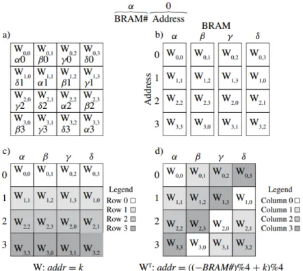
The first implementation is done by Ly and Chow [68]. They implemented their design on Xilinx Virtex II-Pro XC2VP70 FPGA running at 100 MHz. The resources support an RBM up to 128×128 nodes. Their solution to solve the weight distribution problem is that they distributed the connec-tion weights onto different BRAMs in a way that no embedded RAM will simultaneously read out two or more elements from the same row with the same address, and no embedded RAM will contain two or more elements of the same column. Then by using a carefully designed address scheme, a column or row of the matrix is read out from the memory each cycles and no communication is required for the transpose. This distributed BRAM-based matrix data structure is illustrated in Fig. 2.5 withn = 4. Their architecture uses binary-valued visible node states, which reduce the resource utilization greatly without using any multipliers for multiplication. Since the node states are binary values, the matrix multiplication operations are implemented with a series of AND gates and a binary tree adder to calculate the partial ener-gies. To further simplify their implementation, they use a threshold function for node selection.
Figure 2.5: (a) Typical weight matrix organization with BRAM addresses added, (b) weight assigned to BRAMs, (c) weights access by row, (d) weights access by column
of an RBM running on a 2.8 GHz Intel processor. Their implementation was able to achieve computational speed of 1.02 billion connection-updates per second and a speed-up of 35 fold compare to a software implementation.
2.2.2
Sub-Row Memory Core
The second implementation is done by Kim et al. [67], where they designed a highly scalable RBM on FPGA. They implemented their RMB architecture on an Altera Stratix III EP3SL340 FPGA with a DDR2 SDRAM interface. The Altera Nios II soft-processor is also used and running at 100 MHz while the RBM module ran at 200 MHz. Unlike the first implementation, their work was capable of supporting both real-valued and binary-valued visible node states. At high level, their RBM module has an array of weights and neurons that are fed into an array of multipliers and adders to perform matrix multiplication. At the lower level, their RBM module is segmented into several groups, with each group consisting of an array of multipliers, adders,
embedded RAM, and logic components. The weights and neurons are also distributed across the network. This implementation makes the design highly scalable since a group can be easily added to the RBM module to increase the size of the RBM model.
Their architecture used 16-bit fixed-point numbers to represent the weight and node probability, which is capable of training RBM without affecting its learning ability. They treated matrix multiplication in several different ways. A matrix multiplication shown in Eq. (2.19) can be considered as multiple linear combinations of vectors, multiple vector inner products, and as a sum of vector outer products as shown in Eq. (2.20), Eq. (2.21), and Eq. (2.22). They achieved performance acceleration by implementing groups of multipliers, adders and embedded RAM. Each group stores a row of the weights stored on separated local memory. The computation hardware is then selected on the type of energy that is being generated using the DSP units. Multiply-and-accumulate logic generates the visible energies while an adder tree is used for the hidden energies. This allows both types of energies to be generated using the identical memory access to avoid the weight transpose problem. C =A·B where A Rm×k, B Rk×n (2.19) C1,j C2,j · · · Cm,j = k X i=1 Bi,j A1,i A2,i · · · Am,i (2.20) Ci,j = h
Ai,1 Ai,2 · · · Ai,k i · B1,j B2,j · · · Bk,j (2.21) C = k X i=1 A1,i A2,i · · · Am,i
×hBi,1 Bi,2 · · · Bi,n i (2.22)
For node selection, a piecewise linear approximation of a nonlinear function was used to create a sigmoid function, which only requires a minimal number of addition and shift operations [76]. The random number generator uses a
combination of a 43-bit Linear Feedback Shift Register (LFSR) and 37-bit Cellular Automata Shift Register (CASR), which provides good statistical properties and a cycle length of 280, which is sufficient for RBM application. They compared their implementation to the MATLAB code provided by Hinton et al. [1] using a 2.4 GHz Intel Core2 processor implemented in a single thread. Implementing network sizes of 256 × 256, 512×512, and 256
× 1024. They achieved speed-up of 25 fold compared to a single-precision MATLAB implementation and 30-fold for a double-precision MATLAB im-plementation.
CHAPTER 3
OUR IMPLEMENTATION OF RBM WITH
ASYMMETRIC WEIGHT
The objective of this thesis is to implement an RBM architecture on FPGA optimized for handwriting recognition. Due to the nature of this application, the neural networks used to train the input data will have very asymmetric connection weights. Each input data vector represents an handwriting image, where each node presents a pixel in the image. The hidden nodes on the other hand represent the 10-bit label of each image, which each hidden node presents 1 bit. As a result, the number of nodes in the visible layer is going to be much larger than the number of nodes in the hidden layer. Initially, the implementation is optimized for the MNIST benchmark where each image is 28 by 28 pixels and the labels for each image is represented using a 10-bit vector. Later in the implementation stage, the architecture is change so the visible layer size can scale to different sizes to train different input image sizes.
Our implementation is capable of supporting both real-valued and binary-valued visible node states. We used 18-bit fixed-point to represent node probabilities and connection weights. There are two reasons for choosing 18-bit fixed-point numbers to be our data type. First, studies have been shown that RBMs can be trained with a minimum of 16-bits. Second, the FPGA that we used for this implementation has abundant 18 ×18 bit embedded multipliers.
To make the implementation simpler, we decide to use that is a negative power of 2 so that the multiplication operations for calculating the delta weight can be implemented by shift operations instead of resource intense multipliers.
Our overall design breaks down into seven big modules: control unit, node selection core, matrix multiplication core, memory core, visible nodes mod-ule, hidden nodes modmod-ule, and I/O interface. This chapter will discuss the design of each module in great detail.
3.1
RBM Core
RBM is the top-level entity of the entire design. It consists of seven modules. 1. Control Unit: This module made up by two state machines, one for the RBM computation, and one for fetching input data from the SRAM. The state machine for RBM computation keeps track of the AGS phases. Depending on the AGS phases, the control unit will gener-ate different control signals to other modules.
2. Node Selection Core: This module computes the probability of a node state to be turned on for a visible and hidden node using a sigmoid function and the partial energy of the hidden layer or visible layer. 3. Matrix Multiplication Core: This core is responsible for any matrix
multiplication operation needed for the RBM algorithm. It consists of an array of multipliers and numerous full bit adders.
4. Memory Core: This core has all the connection weights stored on sev-eral individual on-chip memories. Each row of the weight matrix is stored on a separated RAM block. The implementation is designed in a way that no more than two connection weights in the same column will be access at the same time.
5. Visible Node: This module contains the node probability values for the visible layer at the first and Xth AGS phases. It also contains an array of shift registers that are used as temporary storage for the next input training vector.
6. Hidden Node: This module contains the node probability values for the hidden layer at the first and Xth AGS phases.
7. I/O Interface: This module is responsible for fetching the next input training data from the SRAM while the RBM core is performing com-putation on the current input data. It gives the control unit a signal when data is ready.
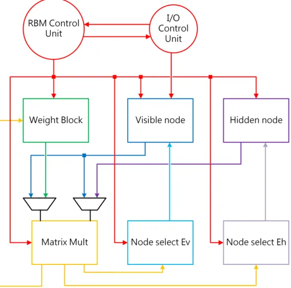
The overall architecture and data flow of the entire design are shown in Fig. 3.1. The control units and their outputs are highlighted in red. As shown in Fig. 3.1, the control signals control all other modules. The outputs
the of weight block, visible node, and hidden node are all inserted into the
M atrix M ult module with two multiplexers. The outputs of M atrix M ult
either feed into the weight block to update the connection weights or feed into the node select module and update the values in visible or hidden layer.
Figure 3.1: A top-level diagram of the RBM core
3.2
Control Units
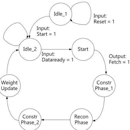
The controlunits module consists of two control units, one for the RBM computation running at 100 MHz and another one for the I/O interface running at 200 MHz. The control unit for RBM computation has seven states as shown in Fig. 3.2.
Figure 3.2: The state machine of RBM computation
1. When the state machine starts or whenever thereset signal is one, the state machine will go to Idel 1 state. The state machine will stay on this state until the startsignal is one, and then to move on the Idle 2 state.
2. In Idle 2 state, the RBM computation core is waiting for the I/O in-terface to finish fetching one input data vector. Once the dataready
from another control unit is one, the state machine will move on to the
start state.
3. During the start state, the data that stored in the shift registers will be loaded into registers that hold the values for visible nodes. At the same time, the control unit sent the I/O interface control unit af etch
signal, so that the I/O interface will start fetching the next input data vector from the SRAM to the shift registers while the computational core is processing the current input data. Without any additional input signals, the state machine will move on to the next state.
the node values for the first AGS phase using Eq. (2.14), Eq. (2.15), and Eq. (2.17). As shown in Fig. 3.3, the connection weights and visible node values are fed into the matrix multiplication core. At each clock cycle, a partial energy Eh is calculated and its value is fed into the N ode selection Eh module. Once the N ode selection Eh module calculates the sigmoid function of the given partial energy, the hidden node will be updated with the new values.
Figure 3.3: A data flow diagram for the construction phase
5. Once the construction phase is finished, the state machine will move to the reconstruction phase. During this state, the computational core is calculating the node value for the second AGS phase using Eq. (2.14), Eq. (2.15), and Eq. (2.16). As shown in Fig. 3.4, the connection weights and the hidden node are fed into the matrix multiplication core. Once all the partial energiesE v are calculated, their values will be fed into the node selection Ev module to compute the sigmoid function. After that, the visible layer will update its node values.
6. Once the reconstruction phase is done, the state machine will move to the second construction phase which calculates the third AGS phase. In this phase, the data flow is exactly the same as the first construction phase.
7. After the second construction phase is finished, the state machine will move to the weight update phase. As shown in Fig. 3.5, the visible
Figure 3.4: A data flow diagram for the reconstruction phase
node and hidden node values from both the first and third AGS phases will be feed into the matrix multiplication core to perform the multi-plication operations using Eq. (2.18). The weights are also fed into the matrix multiplication core to calculated the new weights. Once the new weights are calculated, weight block will update its memory contents accordingly.
Figure 3.5: A data flow diagram for the weight update phase
Unlike the control unit for computational core, the state machine for I/O interface is much simpler. As shown in Fig. 3.6, the state machine only consists of two states, Idle and ReadData. The state machine starts with the Idle state, and spins on that state until the f etchsignal is high. During
the ReadData state, the control unit will generate the address for the data to be read, and store incoming data into a shift register. Each input vector contains 784 of 8-bit words and the I/O bandwidth is only 16 bits, therefore state machine will be spinning on Read Data for at least 392 cycles. Once the input vector is ready, it will generate adataready signal, and move back to the Idle state waiting for another f etch signal.
Figure 3.6: The state machine of I/O interface
3.3
Stochastic Node Selection Design
This module calculates the node value and node state using a sigmoid func-tion and a random number generator. To implement the sigmoid funcfunc-tion is very difficult in hardware. A naive approach requires both exponential functions and division, and these two operations are very expensive to im-plement using hardware. However, the sigmoid function is amenable for hardware implementations. First, the range of the function is bounded in the interval (0, 1). As a result, floating-point representation is not required and can be replace with fixed-point representation. Second, the function has odd symmetry. Thus, computing half of the domain is sufficient to generate the remainder of the domain.
3.3.1
Piecewise Linear Interpolator
Originally, a ROM-based look-up table implementation was used. It is an efficient method to provide reasonable approximation for bounded transfer function. The values for the function are precomputed. Then function is then evenly sampled and the sampled data is stored in an on-chip ROM. This is efficient, but it only provides limited resolution. For a 2 kB on-chip ROM with 32-bit output, can only have 512 sampled entries, meaning there is only 9-bit resolution for input values.
To increase the resolution, we implemented the an interpolation that was proposed by Ly and Chow [68] to increase the resolution by operates on the two boundary outputs of a look-up table. The implementation uses linear interpolator as shown in Eq. (3.1), where (u, v) represent the desired point between points (x0, y0) and (x1, y1).
v = y1−y0 x1−x0 (u−x0) +y0 (3.1) The naive hardware implementation of Eq. (3.1) requires both division and multiplication which utilized significant amount of hardware resources. Thus, rather than calculating the interpolation exactly, a recursive piecewise implementation was used. Knowing the midpoint, which can be found by adding the endpoints and right shift by one, the search point is iteratively compared with the midpoints. This implementation gives a good approxi-mation while using little hardware overhead. Furthermore, the design can be easily pipelined.
This hardware implementation is called the kth Stage Piecewise Linear Interpolator (P LIk), where each successive stage does one iteration of a binary search for the desired point. A comparison of P LI2 and LI and corresponding error is shown in Fig. 3.7. A detailed schematic diagram of the P LIk architecture is shown in Fig. 3.8.
Using the ROM-based look-up table andP LIk, a pipelined, high-precision, and resource efficient sigmoid transfer function was implemented. Using fixed-point input data, the sigmoid function is defined as a piecewise imple-mentation using Eq. (3.2). A comparison between the ideal sigmoid function
Figure 3.7: Comparison and error residuals ofLI and P LI2 [68] the piecewise implementation and the error residuals are shown in Fig. 3.9.
f0(x) = 0, x≤ −8 1−P L, I3(LU T(−x)), −8< x≤0 P LI3(LU T(x)), 0< x≤8 1, x >8 (3.2)
Finally, the results of the sigmoid transfer function is compared with a random number to select the final node state. There are many efficient FPGA implementations of uniform random number generators [77], [78]. A Linear Feedback Shift Register (LFSR) is implemented for this RBM architecture due to its simplicity. The block diagram for the node select module for computing the hidden node states is shown in Fig. 3.10.
Although the node select module for computing visible nodes is very similar to the module used for the hidden nodes, it is much larger compared to the node select module for the hidden nodes. This is due to the fact when partial energies for hidden nodes are computed, the RBM computational core outputs oneEh every clock cycle. Since the node select module forEh is pipelined, thus only one piecewise sigmoid function core is need. When the
Figure 3.8: A schematic diagram of theP LIk [68]
partial energies for visible nodes are calculated, 784 of them are computed in parallel. As a result, the node selected module for Eh contains 784 of the piecewise sigmoid function core. This implementation is later optimized, and will be discussed more in detail in Chapter 4.
3.4
Memory Core
To understand how our implementation resolve weight transpose problem, the key observation required is that matrix multiplications can be viewed as multiple linear combinations of vectors, multiple vectors inner products, or as
Figure 3.9: A schematic diagram of theP LIk [68]
a sum of vector outer products. If the construction phase (V W) is viewed as vector inner products, then each row ofV and each column ofW is multiplied element-wise, followed by a sum reduction. This suggests that each row of
W should be placed in separate on-chip RAMs so that all of these elements can be read simultaneously, as shown in Fig. 3.11(a). For the reconstruction phase, HWT, consider the transposed matrix operation (W HT), and view the operation as linear summation of vectors. This requiers that the jth column vector of W is multiplied by the jth element in a column vector of
HT. This gives the structure of Fig. 3.11(b), which compute multiple visible neurons in parallel. Since at each cycles we only need to read a column vector of W for both phases, the memory layout for the weights can remain the same, and it requires no communication for a transpose operation. In work done be Kim et al. [67], they have a similar implementation to store the connection weights. They placed each column of W onto separated on-chip RAMs while our implementation placed each row of W onto separated on-chip RAMs. Even though the difference between the implementations seems to be insignificant, it makes a huge difference on performance. When Kim et al. [67] designed their implementation, they mostly consider for neural networks with symmetric size. Thus, storing a row or a column of their
Figure 3.10: A schematic diagram of the node select module for computing hidden node
implementation does not make a difference. However, for our design, we are dealing mostly with asymmetric neural networks, where the visible layer is much larger than the hidden layer. Suppose we are storing each column ofW
onto separate on-chip RAMs, we are only able to process ten multiplication operations in parallel. But if we are storing each row of W onto different on-chip RAMs, we are able to process 784 multiplication operations in parallel, that is more than 78 times faster.
3.5
Matrix Multiplication Core
The matrix multiplication core consists of two components: array of multi-pliers and array of adders. Since we are trying to process 784 multiplication operations in parallel, we will need 784 of 18-bit multipliers. Depending on AGS phase, the input multiplexer will select appropriate input from con-nection weight, hidden layer, and visible layers to perform multiplication operations. Once the multiplication operation is performed, the output from the multiply will be feed into array of adders to either perform sum reduction or linear summation of vectors.