Joint Optimization in Supply Chain

(1)

Abstract

ZHOU, XIANG (SEAN). Joint Optimization in Supply Chain. (Under the direction of Xiuli Chao and Shu-Cherng Fang).

(2)

JOINT OPTIMIZATION IN SUPPLY CHAIN

by

Sean Xiang Zhou

A dissertation submitted to the Graduate Faculty of North Carolina State University

in partial fulfillment of the requirements for the Degree of

Doctor of Philosophy

Operations Research

Raleigh, North Carolina

March 2006

Approved By

Dr. Shu-Cherng Fang Dr. Henry L. W. Nuttle Co-chair of Advisory Committee Advisory Committee

Dr. Mihail Devetsikiotis Dr. Xiuli Chao

(3)

Biography

Sean Xiang Zhou was born to Zhuowei Zhou and Congcong Lin on December 25th, 1978 in the city of Xiamen, Fujian Province, China. He spent the first 19 years of his life there before he left for his undergraduate study at Zhejiang University (ZJU), Hangzhou, China.

He was admitted to Zhejiang University in 1997 and majored in Automation (now called System Science and Engineering) in the College of Electrical Engineering. In the four years of study at ZJU, he not only got the knowledge and skill of engineering but also built strong mathematical background, which helps him greatly in the later graduate study and research.

(4)

(5)

Acknowledgment

My parents work very hard to make the life of my brother and myself wonderful. Without their support, I will not be able to achieve anything. I thank my parents and brother for all their love and for everything they have done for me. I also gratefully acknowledge the encouragement, advice and help that I have received from my relatives.

I would like to thank my girlfriend Xinshui (Yancy) Yang, who always has confidence in me and always stay with me to overcome whatever difficulty I face in my daily life during my Ph.D. study.

I have great respect for the teachers at my schools. In addition to being good instruc-tors, they were dedicated and caring. I have enjoyed all the course work at NC State, thank you to the excellent instructions of the faculty.

(6)

I thank Professor Shu-Cherng Fang for being my co-advisor at NC State University. His personal and academic advice during my whole graduate study benefits me a lot. I also thank Professor Henry Nuttle, Mike Devetsikiotis for being my committee members. I am also thankful to Professor Kevin Shang from Duke University, with whom I had opportunity to get involved in some joint research, which is fruitful and very enjoyable. I would like to thank Professor Chung-Yee Lee and Professor Shaohui Zheng from The Hong Kong University of Science and Technology (HKUST) for their kindly help and support during my visit at HKUST in Spring semester of 2005.

(7)

List of Figures

3.1 f(γ, y) and G(y) . . . 17

3.2 r(γ) and r(γ) +Q(γ) . . . 19

3.3 p∗_{(y) and}_{G(y) . . . .} ₂₁

3.4 Optimal R and R+Q . . . 37

3.5 Optimal sγ and ¯Sγ . . . 41

3.6 Properties of optimal p . . . 44

(13)

List of Tables

3.1 u(p) = α+βp2 _{. . . .} ₂₆

3.2 u(p) = eθp _{. . . .} ₂₇

6.1 Three-stage model with batch ordering and fixed replenishment schedule 111

7.1 Optimal and Two Upper Bound Policies: Average Cost . . . 126

7.2 Lower and Upper Bound/Optimal Policies: Discounted Cost . . . 127

(14)

Chapter 1 Introduction

With information revolution, increased globalization and competition, supply chain has become longer and more complicated than ever before. These developments bring supply chain management to the forefront of the management’s attention. Inventories are very important in a supply chain. The total investment in inventories is enormous, and the management of inventory is crucial to avoid shortages or delivery delays for the customers and serious drain on a company’s financial resources.

(15)

tool to balance customer demand and the firm’s inventory.

These developments raise the need and interest of developing models that integrate production decisions, inventory control and pricing strategies. In this study, we discuss several models that combine inventory control or production planning with pricing. We characterize the optimal inventory/production and pricing strategies and develop compu-tational algorithms for the optimal policies. Furthermore, we provide some quantitative and qualitative relationship of the optimal policies and system parameters. After reviwe-ing the literature related to this dissertation in Chapter 2, in Chapter 3, we analyze joint optimization of pricing and inventory control for several continuous-review inventory systems, namely, (Q, r,p) system, batch ordering (R, nQ,p) system and (s, S,p) type system. In these systems, demand arrival rate depends on the price and our objective is to maximize the average profit. In contrast to Chapter 3, we discuss two periodic-review inventory/production models with pricing in Chapter 4. One is production model with production smoothing cost; the other is inventory model with two transportation modes. The demand functions in both models are price-dependent and our objective is to maxi-mize the total discounted profit over finite or infinite planning horizon. We characterize the optimal policies and provide some structure properties of the policy parameters and key performance measures.

(16)

the system. Not only practically but also theoretically, multi-echelon inventory systems are considered as one of the most important classes of models for supply chains. Multi-echelon inventory system includes three major building blocks: serial system, assembly system and distribution systems. Starting from Clark and Scarf (1960)’s seminal paper, many research works have been conducted in analyzing multi-echelon inventory systems with different structures and settings. In this dissertation, we mainly analyze serial system and assembly system.

Delivery time has increasingly become an important measure of service levels for cus-tomers and companies are all trying to respond customer orders in minimum time. But usually quicker response means higher cost. There are different classes of customers who have different delivery time requirements. In Chapter 5, we develop multi-echelon in-ventory models with multiple classes of demand and guaranteed delivery time and we show that echelon base-stock policy is optimal. We also present efficient computational algorithms for determining the optimal control parameters.

In production/distribution systems, material is usually produced/ordered in batches and inventory replenishment between locations often follows a fixed schedule. Large retail chains, such as Wal-Mart, replenish its items in several base quantities and deliver to retailer sites according to a fixed schedule. In Chapter 6, we derive the optimal policy for a serial system with batch ordering and nested replenishment schedule and develop computational algorithm for the optimal policies.

(17)

base-stock levels for the classical serial system with both average cost and discounted cost. Based on these solutions, we derive several newsvendor bounds. Based on these bounds, a simple heuristic for the optimal policies is developed.

Supply chain models with multiple transportation modes have gained momentum in recent years due to the increasing popularity of outsourcing. Cost and leadtime are two important measures of the suppliers for outsourcing. A supplier who provides shorter leadtime usually has higher price. To balance this tradeoff, companies often adopt mul-tiple sourcing strategies by sharing its business with mulmul-tiple suppliers. Consequently, companies need to strategically determine the ordering quantity from each supplier based on its inventory status and demand forecast in order to minimize cost. The strategic im-portance of utilizing multiple suppliers with long and short lead time was first recognized by the US fashion industry. Many firms in this sector have moved their major man-ufacturing facilities offshore to take advantage of the lower production cost. However, some still prefer to maintain costly domestic facilities so that they can better respond to changes in market demand. The combination of ‘quick-response, or short leadtime’ sup-pliers with ‘low cost, long leadtime’ supsup-pliers has been viewed by many as an appropriate strategy to meet fickle customer demand. In Chapter 8, we study the infinite horizon problem of serial inventory system with two transportation modes between stages. It is known that the optimal stationary policies of this system can be obtained by solving 2N nested convex optimization problems recursively. Despite its simple form, however, it is not easy to see the key determinants of the optimal policy and minimum cost from the recursion. we develop simple newsvendor bounds and heuristics for the optimal inventory control policies that can shed light on the effect of system parameters.

(18)

Chapter 2 Literature Review

2.1 Combined Inventory Control and Pricing for

Single-Stage Inventory Models

In this section, we first review the single-stage stochastic inventory models that are closely related to our work. After that, we go over the literature on joint optimization of pricing and inventory.

(19)

cumulative demand model the steady state inventory position is uniformly distributed and independent of the leadtime demand and the average number of backorder is a convex function of Q and r. Zheng (1992) thoroughly discusses the properties of the (Q, r) system.

Continuous-review (S, s) model is a generalization of (Q, r) system. An (S, s) policy, brings the level of inventory to some point S once inventory level drops to or below s, and orders nothing otherwise. Scarf (1960) proves this policy is optimal for a finite-horizon, periodic-review inventory model with setup cost. He introduces a new class of functions, K-convex functions. To improve the implementability of (S, s) policy, Zheng and Federgruen (1991) propose a simple and efficient algorithm to compute the optimal policy parameters S and s. Feng and Xiao (2000) present a different efficient approach to compute the optimal (S, s) policy.

The (R, nQ) policies, if the inventory level is less than or equal to R, an integer multiple ofQis ordered to bring the inventory level into the interval [R+ 1, R+Q], have been studied by many researchers. Hadley and Whitin (1961) show that the inventory position is uniformly distributed between [R+ 1, R+Q]. Veinott (1965) proves (R, nQ) policy is optimal when the order quantity is restricted to be integer multiples of a given base quantity Q for single-stage inventory model. Zheng and Chen (1992) provide an optimization algorithm and sensitivity analysis.

(20)

balance between adjustment, production and inventory cost. Beckman (1961) studies such a problem in which the cost of changing the production rate, i.e., the smoothing cost, is proportional to the amount of change, the inventory holding and demand backlog cost is linear. The objective of the firm is to maximize the short-run or long-run discounted profit. Sobel (1969) generalizes Beckman’s results under more general assumption of convex expected inventory holding and shortage cost for finite horizon problem. Sobel (1971) further extends the result to the infinite horizon case.

(21)

The traditional inventory models we have reviewed focus on effective replenishment strategies and assume a commodity’s price is exogenously determined. Recently, many researchers develop models that jointly optimize the inventory replenishment and pricing. These models can be divided into two different classes.

The first class of models is Revenue Management which has already been successful applied in the airline, hotel and fashion goods retail industries. At the beginning of the planning horizon, the decision maker has a fixed number of initial inventory, such as seats of the flight, empty rooms in the hotel, etc. He tries to use pricing strategy to maximize his revenue over the finite planning horizon while he cannot replenish inventory during the selling season. For a detail review, we refer to the paper by McGill and Ryzin (1999).

The second class of models is in the coordination of inventory replenishment strate-gies and pricing policies, such that at every decision epoch, the manager needs to decide how much to order from the supplier and what is the selling price for the commodi-ties. This topic, starting with the work of Whitin (1955) who analyzes the newsvendor problem with price-dependent demand, has been the focus of many papers. Federgruen and Heching (1999) extend Whitin (1955) to a multi-period model and characterize the optimal inventory and pricing policy as base-stock list price policy.

(22)

discrete and prespecified prices set, especially for two prices and establish the optimality of (s, d, D, S) policy.

2.2 Multi-echelon Inventory Systems

After reviewing single location inventory models, in this section, we switch to multi-echelon inventory models.

Clark and Scarf (1960) study a serial inventory system with finite planning horizon. The system incurs linear inventory holding cost and shortage cost. They introduce a concept of echelon stock and prove the optimality of echelon base-stock policies. Their proof technique involves a decomposition of multi-stage problem into single-stage prob-lem. This approach guides most of the subsequent literature on multi-echelon inventory studies. In particular, Federgruen and Zipkin (1984) extend the result to the infinite horizon setting. Chen and Zheng (1994) use a lower bound approach to prove the opti-mality of echelon base-stock policy for the average cost criterion. For assembly system, Rosling (1989) provides the conditions under which an assembly system can be equiva-lently converted to a serial system. So under these mild conditions, most results of serial system can be carried over to assembly system.

(23)

shipping and the other for expedited shipping. Muharremoglu and Tsitsiklis (2003) gen-eralize Lawson and Porteus’ second assumption by introducing “supermodular” shipping costs structure and show that the optimal policy is extended echelon base-stock type. There is another related work by Huggins and Olsen (2001), who formulate a two-stage supply chain in which stage 1’s order is always met by stage 2. Under the linear ordering cost for regular production and fixed cost for expedited production, they characterize the optimal policy for both downstream and the whole system.

In Clark and Scarf (1960) model, each stage can order any quantity in every period. Chen (2000) generalizes the model by introducing the batch ordering constraint into each stage and establishes the optimality of echelon (R, nQ) policy. For references on echelon-stock (R, nQ) policies, the reader is referred to De Bodt and Graves (1985), Axs¨ater and Rosling (1993), Chen and Zheng (1994, 1998). For this type of policy, every stage can only place an order which is an integer multiple of the base quantity. And the base quantity at each stage satisfies and an integer ratio constraint, i.e., except the most downstream stage, each stage’s base quantity is an integer multiple of its next downstream stage’s base quantity.

(24)

inter-val. The reorder interval of each stage also satisfies an integer ratio constraint, i.e., each stage’s reorder interval is an integer multiple of its next downstream’s reorder interval.

(25)

Chapter 3 Joint Optimization of Pricing and

Inventory Control for Continuous

Review Inventory Systems

(26)

3.1 (

Q, r,

p

)

Model

This section is organized as follows. In§3.1.1, we introduce the notation and present the model. After that, in §3.1.2, we characterize the optimal pricing policy and inventory control strategy. Furthermore, we present efficient computational algorithms to compute the optimal price and inventory control parameters. In §3.1.3 we discuss a structural property of the optimal price. In §3.1.4 the optimality of (Q, r,p) policy is validated.

3.1.1 Model Description

Consider a continuous review inventory system for a single item. The demand arrives according to a Poisson process whose rate λ(p) depends on selling price p. Let u(p) = 1/λ(p) denote the average demand interarrival time. There is a fixed ordering cost K and unit purchasing costc. As in Federgruen and Heching (1999), Chen and Simchi-Levi (2002) (2003), and Feng and Chen (2002) (2003), we assume that the supply leadtime is 0. The objective is to determine the selling price and the inventory replenishment policy so that the average profit is maximized.

(27)

We assume that the average interarrival timeu(p) is increasing convex inp and that the revenue ratepλ(p) is concave inp. Thatu(p) is increasing inpis clear – the higher the selling price, the longer the average time until the next demand. Thatu(p) is convex im-plies that the rate at which the average interarrival time increases is getting higher as the price increases. We shall further assume, though it is not essential, that limp→0pλ(p) = 0 and limp→∞pλ(p) = 0. The last assumption implies that as selling price goes to infinity, all customers are driven away.

It is known that the optimal policy for this problem is (Q, r,p) (see e.g., Chen and Simchi-Levi (2003)). In this policy the parameter r denotes the reorder point, Q is the order quantity, andp= (p(r+ 1), . . . , p(r+Q)) is aQ-dimensional vector of selling prices associated with inventory levelsr+1, r+2, . . . , r+Q. The (Q, r,p) policy works as follows: As soon as the inventory level reachesr, the firm places an order of sizeQ, and when the inventory level isi, the selling price is set at p(i),i =r+ 1, r+ 2, . . . , r+Q. Under the (Q, r,p) policy, the length of time the inventory level stays atiis exponentially distributed with mean u(p(i)). Thus the inventory level process is a Markov Process. To compute the average profit we use renewal reward theory. A cycle starts every time an order is placed. Then the inventory process constitutes a renewal process with average cycle lengthPr_i₌+_rQ₊₁u(p(i)). The average revenue in each cycle isPr_i₌+_rQ₊₁p(i), the purchase cost is cQ, and the holding and shortage cost per cycle is Pr_i₌+_rQ₊₁u(p(i))G(i). Let v(Q, r,p) be the average profit per unit time for the inventory system. It follows from renewal reward theory that

v(Q, r,p) = −K+

Pr+Q

i=r+1(p(i)−c−u(p(i))G(i))

Pr+Q

i=r+1u(p(i))

. (3.1)

(28)

To find the optimal solution for v(Q, r,p), we introduce an auxiliary function. For a given but arbitrary policy (Q, r,p), we define

ℓγ(Q, r,p) = −K+ r+Q

X

i=r+1

(p(i)−c−u(p(i))G(i))−γ

r+Q

X

i=r+1

u(p(i))

= −K+

r+Q

X

i=r+1

(p(i)−c−u(p(i))(G(i) +γ)), (3.2) where γ is called the dummy profit. It is a simple result from fractional programming (see e.g., Schaible (1995)) that γ is the maximum average profit for the optimization problem (3.1) if and only if maxQ,r,pℓγ(Q, r,p) = 0.

For a given γ let

ℓγ = max Q,r,p

ℓγ(Q, r,p). (3.3)

Since for a given policy (Q, r,p) the auxiliary functionℓγ(Q, r,p) is a decreasing convex

function of γ, so is ℓγ.

To obtain the optimal solution for (3.2) for a given γ, we first compute the optimal

p for given r and r +Q. For i = r + 1, . . . , r +Q, since p(i)−c−u(p(i))(G(i) +γ) is a concave function of p(i), the optimal p(i) can be obtained by taking derivative and setting it to 0,

1−u′(p(i))(G(i) +γ) = 0. Thus we obtain

p(i) = (u′)−1

1 G(i) +γ

(29)

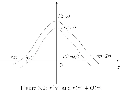
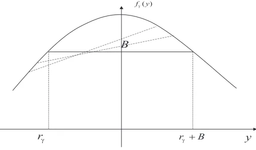
where (u′₎−1 _{is the inverse function of}_u′_{, which is well-defined since} _u′_{is increasing. Note} that p(i) depends onγ even though we have made the dependency implicit. To find the optimalr and r+Q, we define a functionf(γ, y) as

f(γ, y) = p(y)−c−u(p(y))(G(y) +γ) (3.5) wherep(y) is given by (3.4). Clearly, y can only take integer values in (8.2). However in what follows we relax this to allowy to take any real value. In the following discussion, we usef′

1(γ, y) to denote the derivative off(γ, y) with respect toγ andf2′(γ, y) to denote the derivative of f(γ, y) with respect to y. Let R be the set of real numbers.

Lemma 3.1.1 (i) For any given γ >0, f(γ, y) :R → R is a unimodal function ofy, and y0 = 0 is its maximum point.

(ii) For any given y, f(γ, y) is a decreasing concave function of γ.

Proof. We first prove (i). Taking derivative of f(γ, y) with respect to y yields

f₂′(γ, y) = p′(y)−u′(p(y))p′(y)(G(y) +γ)−u(p(y))G′(y) = −u(p(y))G′(y)

where the second equality follows from the fact that f′

2(γ, y) is evaluated at the optimal price p which satisfies u′_{(p(y)) = 1/(G(y) +} _{γ). Because} _{u >} _0, _f′

2(γ, y) is positive (negative) whenever G′_{(y) is negative (positive). Thus it follows from the convexity of} G(y) and lim|y|→∞G(y) = ∞ that f(γ, y) is unimodal in y, and the maximum point of f(γ, y) is the minimum point ofG(y), which is 0.

We next prove (ii). We denote by p′

(30)

0 y )

, ( y f J

) (y G

Figure 3.1: f(γ, y) and G(y)

that the first two derivatives of f(γ, y) with respect to γ are

f₁′(γ, y) = p′−u′(p)p′(G(y) +γ)−u(p) = −u(p),

f₁₁′′(γ, y) = −u′(p)p′_γ(y)

= u

′_(p)

u′′_{(p(y))(G(y) +}_γ)2,

where the second equality follows fromu′_{(p) = 1/(G(y) +}_γ_{) and the last equality follows} from

p′γ(y) =

(u′)−1

1 G(y) +γ

′

= − 1

u′′_(u′₎−1 1

G(y)+γ

1

(G(y) +γ)2 .

Thus it follows from the increasing convexity ofu(p) thatf(γ, y) is decreasing concave

inγ.

(31)

Remark 1. One might expect f(γ, y) to be a concave function of y. We point out that this is not true in general.

Let

ℓγ(Q, r) = max

p

ℓγ(Q, r,p).

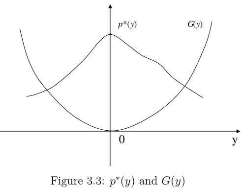
We next characterize the optimalr(γ) and Q(γ) that maximize ℓγ(r, Q) for a given γ.

Lemma 3.1.2 (i) Given γ, the optimal r(γ) and r(γ) +Q(γ) are given by

r(γ) = max{y ≤0 and integer:f(γ, y)≤0} (3.6) r(γ) +Q(γ) = max{y ≥0 and integer:f(γ, y))≥0} (3.7)

(ii) r(γ) is increasing in γ.

(iii) r(γ) +Q(γ) is decreasing in γ.

Proof. Note the relationship

ℓγ(r, Q) =−K+ r+Q

X

i=r+1

f(γ, i). (3.8)

Since f(γ, i) is a unimodal function, the optimal solution for maxr,Qℓγ(r, Q) should be

ther andQsuch thatf(γ, r+ 1), . . . , f(γ, r+Q) are all nonnegative. This proves (i). By Lemma 3.1.1, f(γ, y) is a decreasing function of γ. Hence it follows from the definition of r(γ) and r(γ) +Q(γ) that r(γ) is increasing in γ, and r(γ) +Q(γ) is decreasing in γ.

(32)

) , ( y f J

0

) , ' ( y f J

)

(J

r _r(J') _r(J')_Q(J') r(J)Q(J) y

Figure 3.2: r(γ) and r(γ) +Q(γ)

visualized in Figure 2.

We are now ready to present the main result of this section.

Theorem 3.1.1 The optimal inventory and pricing strategy (Q∗_{, r}∗_,

p∗) is

r∗ = max{y≤0 and integer:f(γ∗, y)≤0} (3.9) r∗+Q∗ = max{y≥0 and integer:f(γ∗, y)≥0} (3.10)

and

p∗(i) = (u′)−1

1 G(i) +γ∗

, i=r∗+ 1, . . . , r∗+Q∗, (3.11)

where γ∗ _{is the optimal average profit determined by}

r∗₊_Q∗ X

i=r∗₊₁

f(γ∗, i) = K. (3.12)

(33)

analysis. Equation (3.3) can be expressed as

ℓγ =−K+

r(γ_X)+Q(γ)

i=r(γ)+1

f(γ, i).

Since ℓγ is a strictly decreasing convex function of γ, ℓγ = 0 has a unique solution γ∗,

which is given by (3.12). Therefore, from the result of fractional programming (see e.g., Schaible (1995)), the proceeding argument guarantees the optimality of the solution.

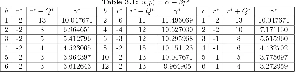
One interesting feature of optimal pricing is its dependency on the inventory level. Federgruen and Heching (1999) prove that for their model the optimal price decreases as the inventory level increases. This does not hold in our model. The following result presents the qualitative relationship between pricing and inventory level in our model.

Theorem 3.1.2 The optimal selling price p∗_(y) _{is increasing on} _r∗ _{+ 1} _≤ _y _≤ ₀_{, and}

decreasing on 0≤y ≤r∗₊_Q∗_.

Proof. For convenience we drop the star on p, r, Q and γ. Again we relax y to allow it to take any real value. Recall that p(y) satisfies equation

1−u′(p)(G(y) +γ) = 0. Taking derivative with respect to y yields

−u′′(p)p′(y)(G(y) +γ)−u′(p)G′(y) = 0 and

p′(y) = − u

′_(p)G′_(y)

(34)

0 y

) (y G )

( *y p

Figure 3.3: p∗_{(y) and} _G(y)

Since u(p) is increasing convex, p increases as G(y) decreases, and p decreases as G(y) increases. Because G(y) is convex with minimum point 0, the result follows.

This result shows that the higher the inventory level, the lower the optimal selling price, and the higher the backlog level, the lower the optimal selling price (see Figure 3). An intuitive explanation for this phenomenon is that, when the on-hand inventory is high, the manager should set the selling price low in order to attract more demand to sell the product in stock; while when the backlog level is high, the manager should also set the selling price low but that is for a different reason – to boost demand so that the reorder point can be reached quickly to incur a low penalty cost.

3.1.2 Algorithms

In Theorem 3.1.1, the parameter γ∗ _{represents the maximum average profit for the} in-ventory system. Once γ∗ _{is obtained the optimal strategy follows from (3.9), (3.10) and} (3.11). Sinceγ∗ is determined by (3.12) which can be written asℓγ∗=0, we need to search

(35)

For any givenγ, the (Q, r,p) that maximizesℓγ(Q, r,p) is easily computed from (3.4),

(3.6) and (3.7), and the optimal value ℓγ is determined. If ℓγ = 0 then we know that the

current strategy is optimal. Otherwise, ifℓγ >0 then by the fact that ℓγ is decreasing in

γ we know that the optimal γ∗ _{> γ, and we should increase} _γ _{to search for the optimal} strategy. Similarly, if ℓγ < 0 then the optimal γ∗ < γ, and we should decrease γ to

search for the optimal strategy. This analysis leads to the following bisection algorithm for computing the optimal strategy.

Algorithm I

Step 1 (Initialization)

Let γ1 = maxpλ(p)(p−c) and γ2 = v(1,−1, p(0)). Then ℓγ1 <0 and ℓγ2 ≥0. Let

ǫ >0 be the tolerance level forγ∗_.

Step 2 (Update γ)

Let γ = (γ1 +γ2)/2. Compute the corresponding (Q(γ), r(γ),p(γ)) using (3.4), (3.6), and (3.7). Compute ℓγ(Q(γ), r(γ),p(γ)).

Ifℓγ(Q(γ), r(γ),p(γ)) = 0, then go to Step 3.

Ifℓγ(Q(γ), r(γ),p(γ))<0, thenγ1 =γ;

Ifℓγ(Q(γ),(r(γ),p(γ))>0, then γ2 =γ.

Ifγ1−γ2 ≥ǫ, go back to Step 2; otherwise, setγ = (γ1+γ2)/2 and go to Step 3.

Step 3 (Termination)

Stop. γ∗ ₌_γ_,_r∗ ₌_r(γ),_Q∗ ₌_{Q(γ), and}_p∗ ₌_p_(γ).

(36)

bound for the optimal average profit; hence the value of the auxiliary function is negative, i.e., ℓγ1 < 0; γ2 is the profit for a feasible policy which is a lower bound of the optimal

average profit. So ℓγ2 ≥ 0. Moreover, we specify a small positive number ǫ as the

tolerance level of γ∗_.

In Step 2, we use bisection search method to locate the optimal γ, and update the corresponding optimal (Q, r,p) using Theorem 1. If the ℓγ <0, then the optimal γ∗ is

betweenγ andγ2, so we replace γ1 byγ; otherwise, it is betweenγ1 andγ and we replace γ2 by γ. After we update either γ1 or γ2, we repeat Step 2. If we find a γ that satisfies ℓγ = 0, then we have reached the optimal solution and terminate the algorithm. If the

difference betweenγ1 and γ2 is less than ǫ, we also terminate the program and obtain an ǫ-approximate optimal γ. We use thisγ to compute the corresponding (Q, r) and p.

Because the problem involves continuous optimization, there exists no algorithm that is guaranteed to stop at the exact optimal solution in a finite number of iterations, as is typical in any continuous optimization problem. However, the algorithm terminates at anǫ-approximate optimal solution in a finite number of steps.

To develop our second algorithm for determining the optimal policy, we need the following lemma.

Lemma 3.1.3 If ℓγ(Q, r,p)>0, then γ1 =v(Q, r,p)> γ.

Proof. By definition we have

ℓγ(Q, r,p) =−K+ r+Q

X

i=r+1

(p(i)−c−u(p(i))G(i))−γ

r+Q

X

i=r+1

(37)

Thus

v(Q, r,p)−γ = −K+

Pr+Q

i=r+1(p(i)−c−u(p(i))G(i))

Pr+Q

i=r+1u(p(i))

−γ >0.

This showsγ1 > γ and the lemma follows.

Lemma 3.1.3 states that, if the average profit γ of a policy is not optimal (because ℓγ >0), then the average profit of the current policy γ1 is greater than γ. This suggests

that if we start with the profit γ of a feasible strategy that is not optimal, then we can improve on it. The process can be continued to generate an increasing sequence which converges. This leads to the following algorithm.

Algorithm II

Step 1 (Initialization)

Letγ0 =v(1,−1, p(0)), which satisfies ℓγ0 ≥0. Let ǫ >0 be the tolerance level for

γ∗ _and _n _{= 0.}

Step 2 (Update γ) Compute (Q(γn), r(γn),p(γn)) based on Lemma 3.1.1, and

compute ℓγn(Q(γn), r(γn),p(γn)).

Ifℓγn(Q(γn), r(γn),p(γn)) = 0, then go to Step 3.

If ℓγn(Q(γn), r(γn),p(γn)) > 0, γn+1 = v(Q(γn), r(γn),p(γn)). Set n = n+ 1, If

γn−γn−1 ≥ǫ, go back to Step 2; otherwise, go to step 3.

Step 3 (Termination)

Stop. γ∗ ₌_γ

(38)

The remaining question is whether the point of convergence of this algorithm is the maximum average profit. This is guaranteed by the following result.

Proposition 3.1.1 In Algorithm II, γn converges to the optimal γ∗.

Proof. Since {γn} is an increasing sequence bounded from above by maxpλ(p)(p−c),

it converges to some finite number, say, γ. We need to proveγ =γ∗_{. If this is not true,} then ℓγ > 0. It follows from Lemma 3.1.3 that γ′ = v(Q(γ), r(γ),p(γ)) > γ. Because

v(Q(γ), r(γ),p(γ)) is a continuous function ofγ, for any ǫ >0 such thatγ′₋_{ǫ > γ, there} exists a positive integer N, such that when n > N,

γn+1 =v(Q(γn), r(γn),p(γn))≥v(Q(γ), r(γ),p(γ))−ǫ=γ′−ǫ > γ.

This contradictsγn+1 ≤γ. Therefore γn →γ∗ and ℓγn →0 as n → ∞.

(39)

3.1.3 Numerical Studies

In this section, we provide several numerical examples to illustrate the properties of the optimal pricing strategies. Two particular forms of u(p) are considered: u(p) =α+βp2 and u(p) =eθp_.

In Table 1, u(p) = α+βp2 _with _α _{= 0.05,} _β _{= 0.005 and} _K _{= 20. We present} the optimal r∗_, _r∗ ₊_Q∗ _{and maximum average profit} _γ∗ _{in the table for the examples} generated by varying the parameters h, b, and c one at a time from base case values of h = 1, b = 10, and c = 1. Because the dimension of the optimal price vector changes as r∗ _and _Q∗ _{change, we do not include the optimal price in the table. We list some} examples here: When h= 3, r∗ ₌₋_{2 and} _r∗₊_Q∗ _{= 5, the optimal price is} _p∗₍₋_1,_{5) =} (6.50,18.50,11.90,8.80,6.90,5.70,4.90); another example, when b = 4, r∗ ₌ ₋_{4 and} r∗_+Q∗ _{= 12, the optimal price is}_p∗₍₋_3,_{12) = (4.40,}_5.40,_6.80,_9.40,_8.60,_7.90,_7.30,_6.80, 6.40,6.00,5.70,5.40,5.10,4.80,4.60,4.40).

Table 3.1: u(p) =α+βp2

h r∗ _r∗₊_Q∗ _γ∗ _b _r∗ _r∗₊_Q∗ _γ∗ _c _r∗ _r∗₊_Q∗ _γ∗

1 -2 13 10.047671 2 -6 11 11.496069 1 -2 13 10.047671

2 -2 8 6.964651 4 -4 12 10.627030 2 -2 10 7.171130

3 -2 5 5.412796 6 -3 12 10.295968 3 -1 8 5.515960

4 -2 4 4.523065 8 -2 13 10.151128 4 -1 6 4.482702

5 -2 3 3.964397 10 -2 13 10.047671 5 -1 5 3.775697

6 -2 3 3.612643 12 -2 13 9.964905 6 -1 4 3.272959

In Table 2, u(p) takes the form u(p) = eθp _with _θ _{= 0.05 and} _K _{= 30. The base}

(40)

Table 3.2: u(p) =eθp

h r∗ _r∗₊_Q∗ _γ∗ _b _r∗ _r∗₊_Q∗ _γ∗ _c _r∗ _r∗₊_Q∗ _γ∗

1 -1 3 3.211318 2 -2 3 3.442351 1 -1 3 3.442247

2 -1 2 2.367485 4 -1 3 3.211318 2 -1 3 3.211318

3 -1 1 1.986400 6 -1 3 3.211318 3 -1 3 2.998423

4 -1 1 1.725084 8 -1 3 3.211318 4 -1 3 2.791912

5 -1 1 1.518209 10 -1 3 3.211318 5 -1 3 2.596384

6 -1 0 1.485544 12 -1 3 3.211318 6 -1 3 2.415886

From Tables 1 and 2, the following observations can be easily made and verified. First, the optimal order-up-to level r∗ ₊_Q∗ _{is decreasing in the unit holding cost rate} _h _and the linear purchasing cost c, but it is increasing in the unit backlog cost rate b. Second, the optimal reorder point r∗ _{is independent of the holding cost rate} _{h, which is because} r∗ _<_{0, but}_r∗ _{is increasing in}_{b. However, since the demand follows a Poisson process and} order leadtime is 0,r∗ _{is always less than 0. Hence,} _r∗ _{remains constant at} ₋_{1 after some} level of b. Third, the optimal profit decreases as the cost parameters increase. Fourth, it can be proved analytically that, in these examples the rate of decrease in p∗_{(y) gets} smaller with positive, increasing values of y, and the rate of increase in p∗_{(y) gets larger} with negative, increasing values of y. This interesting property, however, does not hold for general u(p).

3.1.4 Optimality Verification of

(

Q, r,

p

)

Policy

The policy (Q∗_{, r}∗_,_p∗_{) obtained in the previous algorithm (we will omit the} _∗ _{in the} following proof) is optimal among all the feasible policies if this policy and its long-run average profit R∗ _{together satisfy the following} _{long-run average profit criterion}_:

h(x) = sup

y≥x,p∈[c,∞)

(

−Kδ{y > x} − G(y) +R

∗ λ(py)

+ (py−c) +h(y−1)

)

(41)

whereh(x) must be a bounded function. So we relax the original problem to the following problem which is allowed to return some unsold goods:

h(x) = sup

y6=x,p∈[c,∞)

(

−Kδ{y6=x} −G(y) +R

∗ λ(py)

+ (py −c) +h(y−1)

)

where δ(A) = 1 if the A is true, and otherwise it is 0.

As will be shown later in this section, it turns out that the optimal solution to the relaxed formulation stipulates a (Q, r,p) policy for inventory management and pricing. Specifically, when the inventory level of goods is abover+Q, the retailer may return the inventory in order to bring the inventory down to r+Q. As a result of returning goods, it will never happen more than once since after that the inventory level will always at or below r+Q. Therefore, for the criterion of long run average profit, if we follow the same policy for the original problem with no good-returning allowed, the same long run average profit will be achieved and it must be optimal for the original problem too. This technique was first employed in Zheng (1991).

Now we need to construct a bounded functionh(x) that satisfies the optimality equa-tion. We will structure the function in relation to the auxiliary function ℓv(Q, r,p). In

the following proof procedure, we will change the notation ofℓv(Q, r,p) toℓv(r, r+Q,p)

for convenience.

A functionh(x) is defined recursively as follows:

h(x) =

    

   

−K if x≤r,

ℓv(r, x, p(r+ 1, x)) if r < x≤r+Q,

max{−K,maxp{−G_λ(x₍_p)+₎v + (p−c) +h(x−1)} if x > r+Q.

(42)

Now it is obviously true that −K ≤ h(x) ≤ 0 when x ≤ r. For x > r +Q, h(x) ≥ −K. Consider the case when x ∈ (r, r +Q]. As (Q, r,p) optimizes ℓv(r, Q+r,p), so

ℓv(r, x, p(r, r+x))< ℓv(r, r+Q,p) = 0 when x > r.

In the following we showh(x)≥ −K when r < x≤r+Q: h(x) = ℓv(r, x, p) = −K+

x

X

i=r+1

(pi−c−u(pi)(G(i) +v))

≥ −K

Because λ(px−i)(px−i−c)−G(x−i)−v ≥0 by the definition of the optimal r and Q.

Now we proceed to the case that x > r +Q, we prove it by induction, start from x=r+Q+ 1, if h(r+Q+ 1) =−K, then it is automatically satisfied, otherwise:

h(r+Q+ 1) = max

p

(

−G(r+Q+ 1) +v

λ(p) + (p−c) +h(r+Q+ 1−1)

)

≤ max

p

(

−G(r+Q+ 1) +v

λ(p) + (p−c)

)

≤ 0

The first inequality follows from the previous results and the second is based on the definition of r +Q. The induction procedure is simple so we omit it here. So far,

−K ≤h(x)≤0.

After we showh(x) is bounded, we need to show it satisfies the dynamic programming equation above. We will discuss several cases separately.

Forx≤r:

We need to show −K ≥ −G_λ(₍x_p)+v

(43)

definition of r:

G(r)> λ(p)(p−c)−v so with x−1< r and h(x−1) =−K

−G(x) +v

λ(px)

+ (px−c)−K ≤ −K

so h(x) = −K satisfies the optimality equation.

Forr < x≤r+Q, We prove the result by induction, let x=r+ 1 then

h(r+ 1) = (pr+1−c)−

G(r+ 1)−v λ(pr+1)

−K = ℓv(r, r+ 1, p(r+ 1))

Suppose the this is true for x=i, then for x=i+ 1

h(i+ 1) = −G(i+ 1) +v

λ(pi+1)

+ (pi+1−c) +h(i) = −G(i+ 1) +v

λ(pi)

+ (pi+1−c) +ℓv(r+ 1, i, p(r+ 1, i))

= ℓv(r, i+ 1, p(r+ 1, i+ 1))

Therefore, we finish the induction and prove this case.

Finally, we prove theh(x) we constructed is valid for range x > r+Q. We just need to verify in this range, h(x) is equivalent to:

max

(

−K,max

p {−

G(x) +v

λ(p) + (p−c) +h(x−1)

)

(44)

3.2 Batch Ordering (

R, nQ,

p) Model

In this section, we consider a continuous-review inventory model, in which demand arrives according to a batch Poisson process. The demand arrival rate depends on the selling price while the demand size does not. In addition, the ordering quantity must be an integer multiple of a base quantity Q. We characterize the optimal inventory and pricing policies. We also present how to calculate the control parameters and obtain a structural property for the optimal price.

3.2.1 Model Description

Consider a continuous-review, single-stage inventory system. Demand arrives according to a batch Poisson process. The demand size is i.i.d. with distribution φ(·) and mean µ. The interarrival time is exponential distributed with rate λ(p), which depends on the selling price. The firm needs to make pricing as well as the inventory replenishment decisions. Assume the supply leadtime is 0 and unsatisfied demand is fully backlogged. Let x denote the initial inventory level andy denote the inventory level after replenish-ment. The inventory holding and shortage cost function is G(y), which is a function of the inventory level after replenishment. The unit purchasing cost is c. When the firm places an order, the order quantity is an integer multiple of a given base quantity Q.

The time sequence of the events is: First, demand arrives and is satisfied if the inven-tory is enough, otherwise it is backordered; second, the firm decides whether to place an order and if so, how much to order to replenish its inventory; third, the firm determines the selling price for the product; fourth, all costs and revenue are incured.

(45)

be the minimum point of G(·);

Assumption 3.2.2 u(p) = 1/λ(p) is a convex function ofp and it is strictly increasing in p.

The objective of the firm is to maximize its long run average profit per unit of time. We consider the following (R, nQ,p) policy: If inventory level drops to or belowR, place an order which is an integer multiple of Qto raise inventory level to some point between R+ 1 and R+Q; otherwise do not order anything. The optimal price is a function of inventory level.

We first derive the average profit function for a given (R, nQ,p) policy. Letπ(i) denote the stationary probability for the inventory level to beiif the length of inter arrival time is exact one unit. Then

π(0) =π(0) ∞ X k=0 φ(kQ) + Q−1 X j=1 π(j) ∞ X n=1

φ(−j +nQ),

π(i) = i X j=0 π(j) ∞ X k=0

φ(i−j +kQ) +

Q−1

X

j=i+1 π(j)

∞

X

n=1

φ(i−j+nQ),

where π(Q−1) =PQ_j₌₀−1π(j)P∞_k₌₀φ(Q−1−j+kQ). Display it in the matrix form as:

π=π         P∞

k=0φ(kQ)

P∞

n=1φ(−1 +nQ)

P∞

n=1φ(−2 +nQ) · · ·

P∞

n=1φ(−(Q−1) +nQ)

P∞

k=0φ(1 +kQ)

P∞

k=0φ(kQ)

P∞

n=1φ(−1 +nQ) · · ·

P∞

n=1φ(1−(Q−1) +nQ)

..

. ... . . . ... ...

P∞

k=0φ(Q−1 +kQ) · · · ·

P∞

k=0φ(kQ)

(46)

It can be easily seen that the matrix is doubly stochastic. so

π(i) = 1 Q

Hence it follows from the theory of Semi-Markov process (Ross, 2003) that the stationary probability of inventory level at i is:

πi =

1/(λ(pi)Q)

PR+Q

j=R+1(λ(pj)Q)

i=R+ 1, . . . , R+Q

where pi is the price when the inventory level is i.

Let v(R,p) be the optimal average profit. Since the base quantity Q is given, we suppress it inv to simplify the notation. Thus the average profit per unit of time is given by:

v(R,p) =

R_X+Q

i=R+1

(πi)(λ(pi)(pi−c)µ−G(i))

=

PR+Q

i=R+1 λ(1pi)(λ(pi)(pi−c)µ−G(i)) PR+Q

j=R+1 1

λ(pj)

(3.13)

We want to maximize the above function, with respect to both R and p. Since this function is not easy to optimize directly, in the following we again introduce an auxiliary function as the tool to simplify the optimization procedure.

We define the auxiliary profit function as follows:

ℓγ(R,p) = R_X+Q

i=R+1 1 λ(pi)

(λ(pi)(pi−c)µ−G(i)−γ) (3.14)

whereγ is the dummy profit. This is a fractional programming expression of the average profit of function (3.13). Again from the result of fractional programming,γ =v∗_{, where} v∗ _{is the optimal profit, if and only if} _ℓ

(47)

When the dummy profit γ is the long-run average profit of a known policy (R0,p0), we can interpret above function (3.14) as follows. Asγ =v(R0,p₀),γ can be regarded as the reference profit per period which will be earned when policy (R0,p0) is implemented. As a result, the auxiliary function can be viewed as an indicator of the comparative performance of policy (R,p).

3.2.2 Optimal

(

R, nQ,

p

)

Policy

Before we proceed, first we introduce a function f(y):

f(y) = max

p

(

1

λ(p)(λ(p)(p−c)µ−G(y)−γ)

)

. (3.15)

Lemma 3.2.1 f(y) is a unimodal function of y, so there exists one point y0 which max-imizes f(y).

Proof. As u(p) = 1/λ(p) and

g(y, p) = 1

then the optimal pshould satisfy the following first order necessary condition:

g′_p(y, p) = µ−u′(p)(G(y) +γ) = 0

⇒ µ=u′(p)(G(y) +γ). Take derivative of f(y) with respect to y,

(48)

where the second equality follows from the fact that f′_{(y) is evaluated at the optimal} price pand optimal pricep needs to satisfy previous equation. BecauseG(y) is a convex function,G′_{(y) is first negative then positive. In addition,}_u(p)_≥_{0. So}_f′_{(y) is first} pos-itive then after some point it becomes negative, which means thatf(y) is first increasing then after some point it will decrease. So it is a unimodal by the definition. Therefore,

there exists a maximum point y0.

Proposition 3.2.1 If u(p) is convex in p, then the optimal price p∗ _{has such property}

that it is increasing when inventory level is less than x0 and decreasing when inventory level is greater x0, where x0 is the minimum point of G(·).

Proof. Take derivative of µ=u′_{(p)(G(y) +}_{γ) with respect to} _y,

u′′(p)p′(G(y) +γ) +u′(p)G′(y) = 0

p′G′(y) =− u

′_(p)(G′_(y))2 u′′_{(p)(G(y) +}_γ).

Because λ(p) is strictly decreasing in p, u(p) will increase inp. Therefore, u′_(p)_>_{0. In} addition, since u(p) is convex in p, u′′_(p) _> _{0. So that} _p′_G′_(y) _< _{0, which means that}

when G′_(y)_>_0, _p′ _<_{0, vice versa.}

This property is quite intuitive: When inventory level is positive, the higher the inventory, the lower the selling price. When inventory level is negative (backlog), the higher the inventory level, the higher the selling price. Or, the higher the backlog level, the lower the selling price.

(49)

Rγ as follows:

Rγ = max{x:f(x+Q)≥f(x)}

Proof. Suppose the price for inventory level in [R+ 1, R+Q−1] are the same for the two policies (R,p) and (R−1,p′_{). Then the optimal reorder point can be located in the} following way:

ℓγ(R)−ℓγ(R−1) =

1 λ(pR+Q)

(λ(pR+Q)(pR+Q−c)µ−G(R+Q)−γ)

− 1

(λ(pR)

(λ(pR)(pR−c)µ−G(R)−γ)

= f(R+Q)−f(R)≥0

Because we already showed that f(y) is unimodal, so above inequality is well defined.

Then we can locate the optimal Rγ easily.

Theorem 3.2.2 Suppose we already pinpoint the R at Rγ for a given γ, then we can

decompose the price optimization procedure of Q prices in to Q one price optimization problem and we can solve it in real time independently as follows, fory=R+1, . . . , R+Q:

p(y) =u−1 µ G(y) +γ

!

Proof. Note that

pγ(y) = arg max

(

1

)

.

By taking derivative of the objective function with respect to p, we can get the desired

(50)

) (y fg

B

g

r rg +B y

Figure 3.4: Optimal R and R+Q

So now we already know how to optimize the auxiliary function for a givenγ, we can easily obtain the optimal Rγ and prices for inventory level fromRγ+ 1 toRγ+Q. Next

we show how to upgrade the dummy profit and finally get the optimal average profit per unit of time v∗ _{, the optimal reorder point} _R _{and price vector} _p_.

Clearly, policy (R0,p0) is not optimal if and only if (Rγ,p(Rγ+1, Rγ+Q)) outperforms

it with respect to the objective functionℓγ(Rγ,p). Thus the end of searching an optimal

(Rγ,p) is either a better alternative or a conclusion that current policy we have is optimal.

However, the following lemma shows that a better alternative need not to be optimal.

Lemma 3.2.2 Suppose that ℓγ(R,p)>0, then,γ1 =v(R,p)> γ.

Proof. The proof is parallel to Lemma 3.1.3, so we omit it.

(51)

Lemma 3.2.3 Suppose for someγ, ℓγ(R,p) = 0, then we already find the optimal policy

(R,p), and v∗ =γ.

3.2.3 Algorithm

Since we already know R∗ _<_max

p{λ(p)(p−c)µ}, so if we let γ1 = maxp{λ(p)(p−c)µ−

G(y)}, and γ2 = c(x0,p). Then,ℓγ1(Rγ1,p) < 0 and ℓγ2(Rγ2,p) > 0. Therefore we can

use bisection method to search the optimal R∗ _{because we can locate the corresponding} optimalRγ and the optimal price easily for any givenγ. Let ǫ be the tolerance level.

Algorithm:

• Step 1: Initialization, set γL=γ1 and γU =γ2;

• Step 2: Set γ = (γL₊_γU_{)/2, search the corresponding optimal} _{R, continue;}

• Step 3: Price optimization: for each i=R+ 1, . . . , R+Q: pi = (u′)−1

µ G(i) +γ

.

• Step 4: Calculate

ℓγ = R_X+Q

i=R+1

((pi−c)µ−u(pi)(G(i) +γ)).

if ℓγ >0, then γL =γ, otherwise γU = γ. go to step 2. If ℓγ = 0 or γu−γL < ǫ,

go to Step 5;

(52)

It is the fact that the bisection search is very efficient, so the algorithm converges very fast and get theǫ-optimal solutions.

3.3 (

s, S,

p

)

Model

3.3.1 Model Description

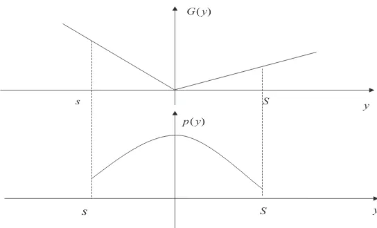
In this section, we study a continuous-review inventory system with setup cost for each order. Again the demand arrives according to a compound Poisson process. The demand size isiwith distributionφ(i) and meanµ. In addition, the demand arrival rateλdepends on the selling price p, i.e. λ(p). The firm determines the selling price and the inventory replenishment strategies. Let K denote the setup cost and c denote the unit purchasing cost. And the inventory holding and shortage cost is G(y). The firm wants to determine the policy that maximizes the long run average profit.

If the mean of interarrival time is 1 unit, then the stationary probability of inventory level atS−i is m(i),

m(0) = 1 1−φ(0), m(i) =

i

X

j=0

m(j)φ(i−j).

For the general case when the arrival rate isλ(pi), the stationary probability of inventory

level at point i, which depends on the selling price will be:

πi =

1/λ(pi)m(i)

PS−s−1

j=1 1/λ(pj)m(j)

,

(53)

is pj.

The average profit per unit of time is

v(s, S,p) = −K+

PS−s−1

i=0 λ(p1S−i)m(i)(λ(pS−i)(pS−iµ−cµ)−G(S−i)) PS−s−1

j=0 1

λ(pS−j)m(j)

. (3.16)

Again we construct an auxiliary function

ℓγ(s, S,p) =−K+ S_X−s−1

i=0 1 λ(pS−i)

m(i)(λ(pS−i)(pS−iµ−cµ)−G(S−i)−γ)

where γ is the dummy profit. Based on lemma 3.1.1, the optimal profit R∗ ₌ _γ _{if and} only if ℓγ(s, S,p) = 0

3.3.2 Optimal

(

s, S,

p

)

Policy

In this section, we compute the optimal (sγ, Sγ,p) that minimizelγ(sγ, Sγ,p) for a given

γ by using the auxiliary function.

Theorem 3.3.1 For any given γ, let a= maxp{(p−c)λ(p)}

(a) the optimal reorder point:

sγ = sup{y:G(y)≥aµ−γ, y < y0}

(b) the upper bound for the order up to point Sγ:

(54)

) (y G

y

g m

-a

g

S

g

s S_g

Figure 3.5: Optimal sγ and ¯Sγ

(c) The optimal price, for y=sγ+ 1, . . . , Sγ, is given by

py =u′−1

µ G(y) +γ

!

Proof. For (a), given any fixed S, and suppose p(s, S) is the same at s+ 1, . . . , S for the two policies, then optimal s satisfies the following:

ℓγ(s−1, S,p)−ℓγ(s, S,p) = m(S−s)(λ(ps)(ps−c)µ−G(s)−γ)≥0

which implies

αµ−G(s)−γ ≥ 0,

(55)

This proves (a).

We prove assertion (b) by contradiction. Note that

ℓγ(s, S, p(s+ 1, S)) = −K+ S_X−s−1

i=0 1 λ(pS−i)

m(i)(λ(pS−i)(pS−iµ−cµ)−G(S−i)−γ)

= −G(S)−γ+λ(pS)(pS−c)µ−K(1− S_X−s−1

j=0

φ(j))

+

S_X−s−1

j=0

φ(j)ℓγ(s, S−j, p(s+ 1, S−j)

≤ αµ−γ−G(S)−K(1−

S_X−s−1

j=0

φ(j))

+

S_X−s−1

j=0

φ(j)ℓγ(s, S−j, p(s+ 1, S−j)

< −K(1−

S_X−s−1

j=0

φ(j)) +

S_X−s−1

j=0

φ(j)ℓγ(s, S, p(s+ 1, S)

The following inequality follows:

ℓγ(s, S, p(s+ 1, S)<−K,

as to be shown, an impossible relation. Now, consider a policy (s, s+ 1, p) for a given γ, such that

λ(p)(p−c)µ−G(s+ 1)−γ ≥0 So this policy will be a lower bound onℓγ(s, S,p) as:

ℓγ(s, S,p)≥ℓγ(s, s+ 1, p′) =−K+m(0)

1 λ(p′₎((p

′₋_c)µ₋_γ₋_G(s_{+ 1)}_{≥ −}_K

(56)

Assertion(c) is easy to show because m(j), j = 0, . . . , S −s−1 are independent of p. We assume thatλ(p) is strictly decreasing of p. Therefore, the demand arrival rate λ and pricep is one to one correspondent, for eachp, we can find a correspondingλ. Thus we can take derivative with respect to p of the objective function,

µ−u′(py)(G(y)−γ) = 0

which implies

py =u′−1

µ G(y) +γ

!

Then we can solve for optimal p immediately.

Theorem 3.3.2 If u(p) is a convex function, the optimal price p(y) increases as y in-creases when y ≤ y0, and p(y) decreases after y > y0. That is, the path of the function

p(y) is opposite to the one period cost function G(y).

Proof. The proof is similar to the one in the previous section, we skip it here.

3.3.3 Algorithm

In this algorithm, we assume that a minimizer ofG(y),y0is known and we have calculated the renewal density m(i) off line. The algorithm starts with a policy (s0, S0,p0). One choice of (s0, S0,p₀) is (y0 −1, y0, p0), where p0 is the price entailing f(y0). Then γ0 is the average profit achieved by this policy.

(57)

s S y

) (y G

s S _y

) (y p

Figure 3.6: Properties of optimal p

Let γ = γ0 = v(y0 − 1, y0, p). Compute f(y0 − 1), f(y0 − 2), . . . until some f(y0−n)< γ. Let sγ =y0 −n, y= max{sγ+ 1, x0}. Let ǫ be the tolerance level.

Calculate the p(sγ + 1, y) by previous result and the value of auxiliary function ℓ

then go to step 1.1.

• Step 1(Upgrading the dummy profit)

1.1 (Updating the dummy profit) If ℓ < 0, go to step 1.2. If ℓ > 0, let

γ = P ℓ

S−s−1

i=0 1/λ(pS−i)m(i)) +γ, go to step 1.3. If

ℓ P

S−s−1

i=0 1/λ(pS−i)m(i)) ≤ ǫ, go to

Step 2.

1.2 (Update order up to point)If G(y+ 1)> αµ−γ, go to step 2. Otherwise y=y+ 1, then calculate thep(y) and ℓ. Go to step 1.1.

1.3 (Update reorder point)

if G(sγ + 1) > aµ−γ, sγ = sγ + 1 until G(sγ+ 1) ≤ aµ−γ. If y ≤ sγ set

y=sγ+ 1, again, calculate the optimal pricep and ℓ

• Step 2(Termination)

(58)

3.3.4 Optimality Verification

In this section, we verify that (s, S,p) policy is optimal among all other policies. Even though the optimality of the policy has been proved by Chen and Simchi-Levi (2002 a), we prove it through different approach in this section.

The optimal (s∗_{, S}∗_,_p∗_{) policy (we will omit the} _∗ _{in the following proof) is optimal} among all the feasible policies if this policy and its long-run average profit v∗ _together satisfy the following long-run average profit criterion:

h(x) = sup

y≥x,p∈[c,∞)

(

−Kδ{y−x >0} − G(y) +v

∗ λ(py)

+ (py−c)µ+E[h(y−D)]

)

,

where h(x) must be a bounded function. We relax the original problem to the following problem which is allowing return the inventory:

h(x) = sup

y6=x,p∈[0,∞)

(

−Kδ{y6=x} − G(y) +v

∗ λ(py)

+ (py−c)µ+E[h(y−D)]

)

.

If our policy is optimal for the relaxed problem, it must be optimal for the original problem too. Now what we need is to construct a bounded function h(x) to satisfy the criterion above. We structure the function in relation to the auxiliary functionℓv∗(s, S,p).

A function h(x) is defined recursively as follows:

h(x) =               

−K if x≤s,

ℓv(s, x, p(s+ 1, x)) if s < x≤S

maxp{−G(x)+v ∗

λ(p) + (p−c)µ+E[h(x−D)]} if S < x≤S, max{−K,maxp{−G(x)+v

∗

λ(p) + (p−c)µ+E[h(x−D)]} if x > S

(59)

ℓv(s, S, p) = 0 when x > s. To show h(x)≥ −K in this range, when s < x≤S

h(x) =ℓv(s, x, p) = −K + x−_Xs−1

i=0 1 λ(px−i)

m(i)(λ(px−i)(px−iµ−cµ)−G(x−i)−v∗)

≥ −K,

where λ(px−i)(px−iµ−cµ)−G(x−i)−v∗ ≥0 by the definition of the optimals and S.

Now we proceed to the case when x > S. We prove it by induction starting from x=S+ 1:

h(S+ 1) = max

p

(

−G(S+ 1) +v

∗

λ(p) + (p−c)µ+E[h(S+ 1−D)]

)

≤ max

p

(

−G(S+ 1) +v

∗

λ(p) + (p−c)µ

)

≤ 0

where the first inequality is based on the previous results and the second is based on the definition of S. The induction procedure is simple so we omit it here.

After we show h(x) is bounded, we need to show it satisfies the optimality equation above.

Forx≤s, we need to show −K ≥ −G_λ(x₍)+_p v∗

x) + (px−c)µ+E[h(x−D)], which can be

validated by definition of s:

G(s)>max

p {λ(p)(ps)−c)µ} −v

∗_.

So when x≤s

−G(x) +v

∗ λ(px)

+ (px−c)µ−K ≤ −K

(60)

Fors < x≤S, we again prove it by induction, let x=s+ 1 then h(s+ 1) = (ps+1−c)µ−

G(s+ 1)−v∗ λ(ps+1

+φ(0)h(s+ 1) + (1−φ(0))(−K) which implies

h(s+ 1) = −K+m(0)[(ps+1−c)µ−

G(s+ 1)−v∗ λ(ps+1

] = ℓv∗(s, s+ 1, p(s, s+ 1)).

Suppose that this is true for x=j, then forx=j+ 1

h(j + 1) = −G(j+ 1) +v

∗ λ(pj+1)

+ (pj −c)µ+E[h(j+ 1−D)]

= −G(j+ 1) +v

∗ λ(pj+1)

+ (pj+1−c)µ+

j−s

X

i=1

(φ(i)h(j + 1−i)) +φ(0)h(j+ 1) +

∞

X

i=j−s+1

φ(i)(−K) = −G(j+ 1) +v

∗ λ(pj+1)

+ (pj+1−c)µ +

j−s

X

i=1

(φ(i)ℓv∗(s, j+ 1−i, p)) +φ(0)h(j + 1) +

∞

X

i=j−s+1

φ(i)(−K)

⇒h(j + 1) = m(0)[G(j+ 1) +v ∗ λ(pj+1)

+ (pj+1−c)µ+

j−s

X

i=1

φ(i)ℓv∗(s, j + 1−i, p)

+ ∞

X

i=j−s+1

φ(i)(−K)]

= ℓv∗(s, j + 1, p(s+ 1, j + 1)),

(61)

ℓv∗(s, j + 1, p(s+ 1, . . . , j+ 1)) = −K +m(0)((p_j₊₁−c)µ−

G(j+ 1) +v∗ λ(pj+1)

)

+m(0)

j−s

X

i=1

φ(i)(ℓv∗(s, j+ 1−i, p) +K)

= m(0)((pj+1−c)µ−

G(j+ 1) +v∗ λ(pj+1)

)

+m(0)

j−s

X

i=1

φ(i)(ℓv∗(s, j+ 1−i, p))

+ ∞

X

i=j−s+1

φ(i)(−K).

ForS < x < S we need to show

−G(x) +v

∗ λ(px)

+ (px−c)µ+E[h(x−D)]≥ −K

which can be proved by the definition of S:

−G(x) +v

∗ λ(px)

+ (px−c)µ+E[h(x−D)] ≥ −

G(x) +v∗ λ(px)

+ (px−c)µ−K

≥ −K

Finally, we prove the h(x) is valid for range x > S. We just need to verify that in this range, h(x) is equivalent to:

max

(

−K,max

p {−

G(x) +v∗

λ(p) + (p−c)µ+E[h(x−D)]

)

(62)

3.4 Summary

(63)

Chapter 4 Joint Optimization of Pricing and

Inventory Control for

Periodic-Review Inventory Systems

We study two periodic-review inventory/production models in this chapter. We char-acterize optimal inventory and pricing policies for both models. In §4.1, we consider pricing and inventory strategies for a inventory model with dual supply modes. In §4.2, we combine pricing and production decisions for a production smoothing model.

4.1 Single-Stage Inventory Model with Dual

Trans-portation Modes

(64)

emergency order, the quantity of regular order and the selling price for the product. The leadtime difference between the emergency order and regular order is one period. The objective of the firm is to maximize the total discounted profit over a finite or an infinite horizon.

Time sequence of events is : First, the firm receives the regular order placed in previous period and observes the current inventory level; second, he decides the order quantity by using emergency order and receives it immediately; third, a regular order is placed if needed and the selling price is set; fourth, demand is realized and excess demand is backlogged; fifth, all costs and revenue incur.

4.1.1 Finite Horizon Problem

The following are the notation we need:

xn = the initial inventory level at the beginning of periodn before any decisions are

made;

yn = the inventory level after placing the emergency order;

un= the inventory position after placing the regular order;

T = the length of the planning horizon;

c0 = the unit purchasing cost for regular order;

c1 = the unit purchasing cost for emergency order, c1 > c0;

(65)

Dn(p, ǫ) = the demand in period n and E[Dn(p, ǫ)] = dn(p), where ǫ is the random

perturbation;

G(p, y) = the expected inventory holding and shortage cost, i.e. G(p, y) = E[h[y−

D(p, ǫ)];

pmax, pmin = the lower bound and upper bound of the selling price, respectively;

α= the discount factor, α≤1.

The following assumptions are needed for the deduction of the results:

Assumption 4.1.1 The demandDt(p, ǫ)is concave and decreasing inp. Thus,E[Dt(p, ǫ)] =

dt(p) is concave and decreasing in p.

Assumption 4.1.2 The expected inventory holding and shortage cost per periodGt(y, p) =

E[ht(y−Dt(p, ǫ))] is jointly convex in y and p.

Assumption 4.1.3 The expected revenue function Rt(p) = pdt(p) is concave in p.

Assumption 4.1.4 limy→∞Gt(y, p) = limy→∞[(c1−c0)y+c0u+Gt(y, p)] = limy→∞[(c0−

αc1)u+ (c1−c0)c1)y+Gt(y, p)] = ∞ for all p.

The problem can be formulated as,

vn(xn) = max

un≥yn≥xn,pn∈[pmin,pmax]

{−c1(yn−xn)−c0(un−yn)−Gn(yn, pn) +pd(p)

(66)

Let

fn(yn, un, pn) = −c1yn−c0(un−yn) +R(p)−Gn(yn, pn) +αE[vn−1(un−Dn(p, ǫ)]

(4.2)

and

Vn(xn) = vn(xn)−c1xn

which is equivalent to shift the c1xn to the previous period, and set V0(x) = 0. We can

change (4.1) and (4.2) accordingly,

Vn(xn) = max yn≥xn,pn,rn

{fn(yn, un, pn)} (4.3)

where

fn(yn, un, pn) = (c0−c1)yn−c0un+R(pn)−Gn(yn, pn)

+αE[c1(un−Dn(p, ǫ))] +αE[Vn−1(un−Dn(p, ǫ)]

= (c0−c1)yn+ (αc1−c0)un+R(pn)−Gn(yn, pn)−αc1d(pn)

+αE[Vn−1(un−Dn(p, ǫ)]. (4.4)

4.1.2 Optimal Policies

Theorem 4.1.1 (a) fn(yn, un, pn) is concave with respect to yn, un, pn;

(b) Vn(xn) is concave and nonincreasing in xn.

(67)

p′ ₌_λp

1+ (1−λ)p2, λ∈[0,1] and skip the linear term,

fn(y′, u′, p′) = −G(y′, p′) + (p′ −αc1)d(p′) +αE[Vn−1(u′−D(p′, ǫ)]

= (p′−αc1)d(λp1+ (1−λ)p2)−G(λy1 + (1−λ)y2, λp1+ (1−λ)p2) +αE[Vn−1(λ(u1) + (1−λ)(u2)−Dn(λp1+ (1−λ)p2, ǫ)]

≥ λ((p1−αc1)d(p1)−G(y1, p1) +αE[Vn−1(u1−D(p1, ǫ)])

+(1−λ)((p2−αc1)d(p2)−G(y2, p2) +αE[Vn−1(u2−D(p2, ǫ)])

= λfn(y1, u1, p1) + (1−λ)fn(y2, u2, p2),

where the inequality follows from the concavity and monotonicity of D(p, ǫ), convexity of G(y, p) and the nonincreasingness of V(x). Then by Proposition B4 in Sobel (1984), Vn(x) is concave.

From the optimality equation, Vn(xn) is nonincreasing in xn because the feasible

do-main of yn becomes smaller as xn increases and we are trying to maximize the objective

function.

Therefore, the optimal price is

pn(yn, un) = arg maxp∈[pmin,pmax]{fn(yn, un, pn)}. (4.5)

Lemma 4.1.1 (a) fn(yn, un, pn) is a submodular in y and p;

(b)fn(yn, un, pn) is a submodular in u and p;

Joint Optimization in Supply Chain

Abstract

JOINT OPTIMIZATION IN SUPPLY CHAIN

Biography

Acknowledgment

Contents

List of Figures

List of Tables

Chapter 1

Introduction

Chapter 2

Literature Review

2.1

Combined Inventory Control and Pricing for

Single-Stage Inventory Models

2.2

Multi-echelon Inventory Systems

Chapter 3

Joint Optimization of Pricing and

Inventory Control for Continuous

Review Inventory Systems

3.1

(

Q, r,

p

)

Model

3.1.1

Model Description

3.1.2

Algorithms

3.1.3

Numerical Studies

3.1.4

Optimality Verification of

(

Q, r,

p

)

Policy

3.2

Batch Ordering (

R, nQ,

p) Model

3.2.1

Model Description

3.2.2

Optimal

(

R, nQ,

p

)

Policy

3.2.3

Algorithm

3.3

(

s, S,

p

)

Model

3.3.1

Model Description

3.3.2

Optimal

(

s, S,

p

)

Policy

3.3.3

Algorithm

3.3.4

Optimality Verification

3.4

Summary

Chapter 4

Joint Optimization of Pricing and

Inventory Control for

Periodic-Review Inventory Systems