Explanation of the Most Powerful Copulas and the Proves of Some of Their Properties

(1)

I

nternational

J

ournal of

I

nnovative

R

esearch in

C

omputer

and

C

ommunication

E

ngineering

(An ISO 3297: 2007 Certified Organization)

Vol. 4, Issue 1, January 2016

265 DOI: 10.15680/IJIRCCE.2016. 0401068

Copyright to IJIRCCE

ISSN(Online): 2320-9801 ISSN (Print): 2320-9798

Explanation of the Most Powerful Copulas

and the Proves of Some of Their Properties

Ahmed Al-Adilee

Department of computer Science, Faculty of Education, University of Kufa

ABSTRACT: This paper devoted to review and explain the most common and powerful copula functions in easy and smooth ways. It is an attempt to make the theory of such functions much easier and clear for usage. We firstly demonstrate some basic definitions, properties and concepts related to copula function. Afterwards, we will presentwhat is called thefamilies of copula function and proves some of the properties relate to such families.

KEYWORDS : Joint distribution functions, copulas, inverse functions.

I. INTRODUCTION

Statistical inference of each dependence structure can be demonstrated and fully analyzed by copula function. It plays a central role in the description of dependence structure because it is not only a tool that we used to measure the rate of correlation between two or multivariate random variables, but also because ofits ability to describe the whole dependence structure.

From a historical point of view, copula function was mentioned implicitly in several papers without referring to the name "copula". For instance, Hoeffding bounds in (1940, 1941), which is yet called the maximum and minimum copula, see [3].Frechet has also found new bounds named by his name in 1951. But most of the significant results of copula were published between 1958 to 1976. The major role of copula studies and its applications was shown by Sklar in 1959. He was the first author who uses the word copula in his paper (1959), and his theorem which is named by his name represent the center of the copula theory. One of the most interested results of copula function was published by Fisher in 1997. Another important and impressive name in the world of copula is Nelsen (1993).He extend the range of studies of suchfunction. His book entitled by "Introduction to Copula Function" represents the main reference for many researches who were interested in such topic. In this book, he has collected most common studies of copulas and he also determined many new results, see [3].

Moreover, we can refer to the application of copula function. Nowadays, copula function is an excellent tool in the studies of financial analysis, see [1,4]. It is very important inthe studies of risk management, value at risk, studies of risk modeling, andother financial process. Furthermore, we can figure out that copula has also a wide usage in the biomedical studies and the studies of directional dependence of genes. For instance, usingcopula to describe the interaction between genes, see [2]. There are many other areas of sciencethat need to be investigated with respect to copula, for example, engineering and dynamic studies. Indeed, copula still a fresh idea in the world of statistics and need a much effort to be discussed in different fields of science.

Finally, we refer to the construction of our study that concerns with three main parts. The first part devoted to the essential concepts of copula like definitions, theorems and properties. Second one will show some families of copula. While the third one will focus on the methods of constructing and compiling each type of copula.

II. PRELIMINARIES

(2)

I

nternational

J

ournal of

I

nnovative

R

esearch in

C

omputer

and

C

ommunication

E

ngineering

266 DOI: 10.15680/IJIRCCE.2016. 0401068

and the range of joint distribution function, for more detail, see [1]. We begin with some basic definitions of multivariate copula, and bivariate copula, see [1,3]

Definition 2.1:-Let = [0,1]. For any positive integer number ≥2,a multivariate copula is a function : → that satisfies the following properties

C1. , , … , , … , = 0, if = 0, where , , … , ∈ (grounded).

C2. 1, … , , … 1 = , if all the coordinates are equal to 1 except , where 1 is the greatest element and ≤1.

C3. for all ≤ , ∆ ( )≥0,where is either the lower or upper bound, where = 1,2, … , .

The properties C1, C3 are called the grounded and n-increasing, respectively. In particular, let n=2 so that we can define the bivariate copula function in the following way:

Definition2.2:- A bivariate copula is a function : → that satisfies the following properties

1. For each , ∈ , ( , 0) = (0, ) = 0.

2. For each , ∈ , ( , 1) = , (1, ) = .

3. For each , , , such that ≤ , ≤

( , ) + ( , )− ( , )− ( , )≥0.

Note that the property number three is called the two-increasing property.

We should also refer to the theorem of Sklar which represents the center of the theory of copula function. This theorem was compiled by Sklar in 1959. We can introduced it in a multivariate form as follows:

Theorem 2.1(Sklar's Theorem):-Let ( , , … , )be the multivariatejoint distribution function of the random

variables , , … , withmargins = ( ), = ( ), … , = ( ).Then there exists a multivariate copula

function such that ∀ ∈[−∞,∞]

( , , … , ) = ( , , … , )

if the margins above are continuous then the copula function is unique.We should note that one of the important roles of copula is to describe the joint distribution function ( , , … , )with respect to its margins

( ), ( ), ( ). An important result that we conclude from Sklar's theorem appears in the following proposition:

Proposition 2.1:-Let ( , , … , be a multivariate copula, be the joint distribution function, and , , … , are the margins of . Let ( ), ( ), … , ( )be the inverse of the margins , , … , . Then for any ∈

, = 1,2, … ,

( , , … , ) = ( ), ( ), … , ( ) (1)

Note that using the inverse form in proposition 2.1 is calledthe qausi-inverse technique. Also, it is clear that for = 2, a bivariate form of equation (1) is

( , ) = ( ), ( )

Now, we refer to someexamples of common copulas of two-dimensional and n-dimensional spaces that satisfy the conditions of being copula.

2.1The Product Copula

For bivariate or multivariate independent random variables we obtain this type of copula, denoted by ∏ and defined by the following forms, respectively

∏( , ) = (for bivariate copula).

∏( , … , ) = … (for multivariate copula).

Theorem 2.1.1:- Let , be two continuous random variables. Then , are independent random variables if and only if =∏.

Proof Let , be two independent random variables. Let = ( ), = ( ).

Then, we have ( , ) = ( ), ( ) , but , are independent.

Thus ( , ) = ( ) ( ). Hence ( ) ( ) = ( ), ( )

(3)

I

nternational

J

ournal of

I

nnovative

R

esearch in

C

omputer

and

C

ommunication

E

ngineering

267 DOI: 10.15680/IJIRCCE.2016. 0401068

Therefore =∏= . .

Conversely, let =∏. We know that

∏= . , and this yields that = . . = ( ) ( ) = ( , ).

Therefore, , are independents.

2.2TheMaximumCopula

This type of copula is also called the Frechet-Hoeffding lower bound and is defined by

( , ) = { + −1,0}(for bivariate copula).

( , … , ) = {∑ −1,0}(for multivariate copula).

2.3The Minimum Copula

Indeed, this type of copula is well-known as the Frechet-Hoeffding upper bounds and is defined by

( , ) = { , }, , ∈ (for bivariate copula).

( , … , ) = { , … , }(for multivariate copula).

It has been shown that , and represent the lower and lower bounds of each copula, see [3]. This means that for any copula , we have the following property.

For each , ∈ , ( , )≤ ( , )≤ ( , ).

2.4The Survival Copula

One of the most important types of copulas is the survival copula. For testing the lifetime of components we can see that survival copula is a perfect tool that we could use for analyzing and testing the surviving of item with respect to time . We firstly need to express the meaning of survival distribution function so thatwe can define survival copula.

If ( , )is the distribution function of the random variables , ,with its marginal distribution functions ( ), ( ).

Then the joint survival function of these two random variables is

( , ) = 1− ( )− ( ) + ( , ) (2)

Then, according to equation (2), the survival copula, denoted by is given by

(3) It is not difficult to concludethat satisfies the three essential properties of copula (Definition 2.2).

Connecting to the concept of survival copula we can show an important result associated with the bivariate joint distribution function in the following theorem. But, we firstly need to present the following facts that have been already shown in [3].

Lemma 2.4.1:- Let be a subset of [−∞,∞] . Then S is non-decreasing if and only if for each

( , )∈[−∞,∞] , , ∈ either

1. ∀ ( , )∈ , ≤ → ≤ ; (4)

2. ∀ ( , )∈ , ≤ → ≤ (5)

Lemma 2.4.2:- Let , and be two random variables with joint distribution function . Then is equal to its Fr ́ chet-Hoeffding upper bound if and only if for every ( , )∈[−∞,∞] ,either [ > , ≤ ] = 0, [ ≤ , > ] = 0.

Theorem 2.4.1[3]:- Let ,and be two random variables with joint distribution function . Then is identically equal to its Frechet-Hoeffding upper bound if and only if the support of ia nondecreasing subset of [−∞,∞] .

Now, we are in position to present our theorem that have been mentioned, previously.

Theorem 2.4.2[3]:- Let ,and be two random variables with joint distribution function . Then is identically equal to its Frechet-Hoeffding lower bound if and only if the support of is a nonincreasing subset of [−∞,∞] .

Proof. Suppose that is the support of , and let ( , )be any point in [−∞,∞] . Then the relation (4) holds if and only

if [ < , ≥ ] = 0.Similarly, relation (5) holds if and only if [ ≥ , < ] = 0.

Hence ( ) = [ ≤ ] = ( , ) + [ < , ≥ ],and ( ) = ( , ) + [ ≥ , < ].

(4)

I

nternational

J

ournal of

I

nnovative

R

esearch in

C

omputer

and

C

ommunication

E

ngineering

268 DOI: 10.15680/IJIRCCE.2016. 0401068

2.5 Conditional Copula

This function has a wide range of application in finance, economics, biology, and health insurance companies. In this part, we could present such function with some related concepts. Firstly, it is important to see that Sklar's theorem under a notion of conditionality can lead us to the following proposition, see [4].

Proposition 2.5.1:- Let ( , , ) be a vector of variables where is the given variable. Let , , be the joint, and marginal distribution functions, respectively, and let be a copula. Then each conditional joint distribution function can be defined by its conditional marginal distributions with respect to the copula by the following form

( , | ) = ( | ), ( | ) (6)

By equation(6),we can recall a definition of conditional copula, see [4,5].

Definition 2.5.1:- A bivariate conditional copula is a function : → that satisfies the following properties

1. For each , , ∈ , ( , 0| ) = (0, | ) = 0;

2. For each , , ∈ , ( , 1| ) = , (1, | ) = ;

3. For each , , , , ∈

( , | ) + ( , | )− ( , | )− ( , | )≥0.

where is the given value.

As we have mentioned before, it is clear that property number one and number three are the grounded and two increasing properties, respectively.

For inverse property of Sklar's theorem we present the following proposition, see [3].

Proposition 2.5.2: Let , , | , | , be the copula, joint distribution, and the inverse of the marginal distribution functions, respectively. Then each conditional copula with the two random variables , , and given variable can be explained by an equivalent joint distribution function that is

∀ , ∈ , ( , | ) = | ( ), | ( ) . (7)

where ∈ is corresponding given value of the variable .

Once again, we emphasize that the inverse function in this way is well-known by the quasi-inverse.

Remark 2.5.1:- the structure of any conditional copula depends on the conditional joint distribution function. Mathematically,let ( , , )be a vector of random variables, | be the conditional joint distribution function, be the joint density function of the two random variables , , and be the joint density function of the given variable

so that we obtain the following formula.

| ( , | ) = ( ) | ( , , ) (8)

III. FAMILIES OF COPULA

There are several types of families of copula that we can present in this section with some properties of each family. We can see that each family of copula is classified according to the method of generating it.It is basically classified into two main parts according to their distributions. So when the distribution is not normally distributed, we call the family of copula by non-elliptical copula, otherwise we call copula by elliptical copula.

Indeed, we would show some of these families with respect to the number of parameters of each copula. We begin with non-elliptical copula families, that are:

3.1Non-Elliptical Copula Families

There is a wide range of this type of families. For convenient, we will show the most well-known of them with bivariate forms

3.1.1 The Farlie-Gumbel-Morgentern

Any copula with a quadratic polynomial formbelongs to this family, that has the following form

( , ) = + (1− )(1− ), ∈[−1,1] (9)

This type of copula family with parameter is called a one parameter copula.

3.1.2 Cubic Copula

This family of copula can be obtained by extending a quadratic polynomial form to cubic form. Its formula is defined with respect to two parameters , , and itcan be written by the following form

(5)

I

nternational

J

ournal of

I

nnovative

R

esearch in

C

omputer

and

C

ommunication

E

ngineering

269 DOI: 10.15680/IJIRCCE.2016. 0401068

where, , are functions such that (0) = (1) = (0) = (1) = 0.

3.1.3 Guadras-Auge Copulas

Such family is related to the survival copula. It has been presented in the study of copula families in [3]. Its formula can be reviewed by the following bivariate copula with two parameters

, ( , ) = , , , ∈ (11)

In particular, with = = 0, we obtain, , = , =∏. While, with = = 1, we obtain that , = . Note that

∏, are product and minimum copulas, respectively.

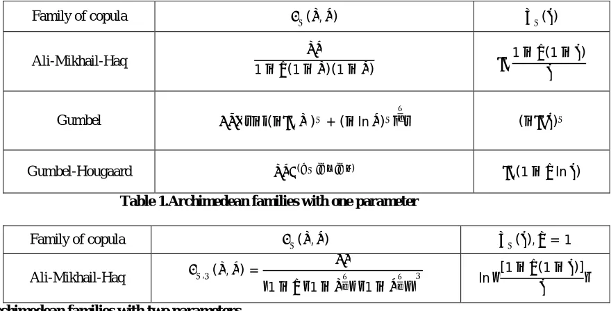
3.1.4 Archimedean Copula Family

This family of copula classified as a non-elliptical family (not normally distributed), and it can be divided into two types depending on the number of parameters that each copula involves. Indeed, each Archimedean copula can be derived from what is called the generator of copula, which differs from copula to another. So, we can present the family of each copula with its generator function, denoted by ( ), in the following two tables.

Family of copula ( , ) ( )

Ali-Mikhail-Haq

1− (1− )(1− )

1− (1− )

Gumbel −(− ) + (−ln ) (− )

Gumbel-Hougaard ( ) (1− ln )

Table 1.Archimedean families with one parameter

Family of copula ( , ) ( ), = 1

Ali-Mikhail-Haq , ( , ) =

1− 1− 1− ln

[1− (1− )]

Table 2.Archimedean families with two parameters

Of course, there are many other families with different generators that can be seen in [3,4,5].

3.2 Elliptical Copula Family

This family of copulas hasonly one general form called the Gaussian copula (normal copula). It belongs to distributions that are elliptically (normally) distributed. In fact, it is defined under distributions, that has a symmetrical tail. And this family has only one specific formula that is, see [3]

C(u, v) =Φρ Φ (u),Φ (v) =

1

2π 1−ρ e

ρ

ρ _dxdy

Φ ( )

∞ Φ ( )

∞

where, −1≤ ≤1, andΦρis the standard two-dimensional normal distribution with 1, 2=0, 1, 2=1.

(6)

I

nternational

J

ournal of

I

nnovative

R

esearch in

C

omputer

and

C

ommunication

E

ngineering

270 DOI: 10.15680/IJIRCCE.2016. 0401068

⋰

IV. METHODS OF CONSTRUCTING COPULA FUNCTIONS

There are several different methods that has been introduced to construct copulas. Indeed, we focus onthe most common of them like Geometric method, algebraic method, Archimedean copulas method, and method of inversion. We show several examples of copula and explain with detail their constructions.

4.1 Geometric Method

This method used to construct copula without reference to distribution functions, or random variables. In other words, it does not depend on the constructions of joint distribution function, or its marginal distribution functions. We could give a particular case, of constructing copulas using the standard definition of copula. This method describes different cases of shapes of copula depending on the type of copula. Indeed, there are two main types of this method as follows:

4.1.1 Singular Copula with Prescribed Support

Each type of copula that has the property of singularity can be constructed by using geometric method. We demonstrate this type by the following examples.

Example 4.1.1:- The copula C whose support (the support of copula is the main diagonal of [0,1]2) consists of the two quarter circles as shown in figure 1. The upper quarter circle is given by u2₊_v2₌_{2u.While the lower one is given by}

u2₊_v2₌_{2v. This copula can geometrically be described according to the following graphs, see [3,4] for more detail.}

4.1.2 Ordinal Sum

Let ( , ) be a copula. Let { } be a collection of copulas with index { }. Then the ordinal sum of { } is given by

( , ) = + ( − )

−

− ,

−

− , ( , )∈

( , ), .

(12)

Again, this ordinal sum of collection of copulascan geometrically be demonstrated in the following figures .

(7)

I

nternational

J

ournal of

I

nnovative

R

esearch in

C

omputer

and

C

ommunication

E

ngineering

271 DOI: 10.15680/IJIRCCE.2016. 0401068

Indeed, there are many other types of copula that can be described under this method such as cover sum, copulas with linear cubic, shuffles of , and so on.

4.2 Algebraic Method

This method has a very important role in constructing copulas. It uses the algebraic relationship between the joint distribution function and its univariate margins in order to construct copula. The theory of this method is based on the following three main rules. For a two dimensional space there are three basic forms, that are, see [3]

1− ( , )

( , ) =

1− ( , )

( , ) (13)

1− ( )

( ) =

1−

(14)

1− ( )

( ) =

1−

(15)

where ( , ) is the joint distribution function, ( ) = , ( ) = are the its marginal distribution functions, and

( , ) is the corresponding copula. In fact, this technique is called Ali-Mikhail distribution. We can demonstrate some

examples that explain the construction of copulas under this method.

Example 4.2.1:- Let and be two random variables with the following distribution function ( , ) = (1 + + ) .

It is clear that ( ,∞) = ( ) = (1 + ) .Similarly, (∞, ) = ( ) = (1 + ) .Then by using the

equations (13), (14), (15) we obtain the following forms

1− ( , )

( , ) =

1−(1 + + )

(1 + + ) =

( )

= +

Also, ( )

( ) = , and

( )

( ) =

This yields the following result

1− ( , )

( , ) =

1− ( )

( ) +

1− ( )

( ) (16)

The corresponding copula function of the formula that we have obtained in equation (16) can be shownin the following example:

Example 4.2.2:- Let and be two random variables with joint distribution function, and its margins,

( , ), ( ) ( ), respectively. Let ( , ) be the copula that we would like to construct, where ( , ) =

( , ), ( ) = , and ( ) = .

According to equation (16) the dependence structure of Ali-Mikhail-Haq (1978), see [4 ]. We obtainthat,

1− ( , )

( , ) =

1− ( )

( ) +

1− ( )

( ) + (1− )

1− ( )

( )

1− ( )

( ) (17)

where is some constant. By using equation (17), we obtain the following construction of copula.

1− ( , )

( , ) =

1−

+1− + (1− )1− 1−

Solve the above equation with respect to ( , ) yields the Ali-Mikhail-Haq family of copula for [−1,1]

Then,

( , )−1 = + + −

(8)

I

nternational

J

ournal of

I

nnovative

R

esearch in

C

omputer

and

C

ommunication

E

ngineering

272 DOI: 10.15680/IJIRCCE.2016. 0401068

1

( , )=

+ − + − + 1− − + − (1− )(1− )

(18)

By rearranging the terms of equation (18)yields the following copula

( , ) =

1 + (1− )(1− )

4.3 Method of Inversion

This method is one of the most importantmethods that have been shown to construct copulas. The interesting way of its form, the properties and the wide range of copulas that lies under it, is the reason that why we are interested in its structure. It has been shown that this method has a bivariate copula, and even a multivariate copula. The main type of this method is well-known by the Marshall-Olkin bivariate exponential distribution, and circular uniform distribution, for more detail, see [4]. Our attention have been paid towards showing the general construction form of each copula, and explain the steps of constructing some of them under this method. We individually present each copula with its name, derivation, and some properties, if they exist. This method basically depends on quasi inverse concept of the marginal distribution function. copulas under this method divided into the following:

4.3.1 Copula with Simple Form

Its form is concluding from the following joint distribution function with domain [−1,1] × [0,∞]

( , ) =( + )∗( −1)

( + 2 −1) (19)

First of all, we need to find the margins of the joint distribution function . This can be done by the following way: Let

= ( ,∞) = ( ) = , = (1, ) = 1− (20)

By solving equation (20) for , , respectively. We obtain

= 2 −1 = ( ), =−ln(1− ) = ( ) (21)

Now, substitute equation (21) in equation (19) to obtain the following copula

∴ ( , ) = ( ), ( ) = ( , ) =(2 −1 + 1)

( )₋₁

2 −1 + 2 ( )₋₁

= [((1− ) )−1]

−1 + (1− ) = ₋_{1 +} = + −

4.3.2 Gumbel's Copula

This copula related to Gumbel's bivariate exponential distribution function that has the following form

( , ) = 1− − + ( ) ₍₂₂₎

The marginal distribution functionsof are:

( ,∞) = ( ) = 1− , and (∞, ) = ( ) = 1−

Now, let

= ( ) = 1− , and = ( ) = 1− (23)

Then, solving equation (23) for , , respectively, yields

=−ln(1− ) = ( ), =−ln(1− ) = ( )

By substituting the equivalent forms of the , above (equation (23)), in equation (22). We obtain that

( , ) = ( ), ( ) = ( , )

= 1− + 1− −1 +

Therefore,

( , ) = + −1 + (1− )(1− ) ( ) ( )

(9)

I

nternational

J

ournal of

I

nnovative

R

esearch in

C

omputer

and

C

ommunication

E

ngineering

273 DOI: 10.15680/IJIRCCE.2016. 0401068

4.3.3 Gumbel-Hougaard Copula

This type of copula directly follows from the following bivariate joint distribution function

( , ) = [ ( ) ] (24)

Of course, the margins of the joint distribution function in equation (24) are

( ) = ( ,∞) = ,and ( ) = (∞, ) =

Let = ,and = , and solve them for ,and ,respectively yieldsthe following forms

= ln(ln ), = ln(ln ) (25)

By substituting the forms of equation (25) in our joint distribution function with property ( , ) = ( ), ( ) , we obtain

( , ) = ( , ) = [−( ( )+ ( )) ] (26)

And by rearranging equation (26), this will lead us to obtain the Gumbel-Hougaard copula. That is

( , ) =

( ) ( )

4.3.4 Ali-Mikhail-Haq Copula

The bivariate joint distribution function of that copula is called the Gumbel'sbivariate logistic distribution. Its formula is

( , ) = [1 + + + (1− ) ] (27)

and its margins are, respectively

( ) = (1 + ) = , ( ) = (1 + ) =

Rearrange ( ), ( ) in equation (27)with respect to , ,respectively. Then

+ 1 = ( ) = , + 1 = ( ) = (28)

Let's write the joint distribution function in equation (27) in the following way

( , ) = (1 + + + 1−1 + (1− ) ) (29)

And substituting equation (28) in equation (29), we have

( , ) = [ + −1 + (1− )( −1)( −1)] (30)

Indeed, the copula in equation (30) can be rearranged so thatwe obtain the general form of Ali-Mikhail-Haq copula. That is

( , ) =

1− (1− )(1− )

4.3.5 Survival Copula

A powerful tool in modern statistical world is the survival copula. its importance appears in testing the lifetime forexamining items in statistical inference, and the easy way for constructing it. Its formula follows from the following general form of joint bivariate survival function. That is

( , ) = 1− ( )− ( ) + ( , ) (31)

Remember that ( , ) = ( , ). Also, we can rewrite equation (31) by the following way:

( , ) = 1− ( ) + 1− ( )−1 + ( , ) (32)

Indeed, we should note that the survival margins of ( , )are

( ) = 1− ( ), ̅_{( ) = 1}₋ ( )

By usingthe forms of the survival margins ( ), ̅( )above, respectively, can lead us to write equation (32) by the following way

( , ) = ( ) + ̅( )−1 + 1− ( ), 1− ̅( ) (33)

By considering that we have : [0,1] →[0,1]as a survival copula such that ( , ) = ( , ). Then from equation (33), we obtain the corresponding survival copula. That is

( , ) = + −1 + (1− , 1− ) (34)

(10)

I

nternational

J

ournal of

I

nnovative

R

esearch in

C

omputer

and

C

ommunication

E

ngineering

274 DOI: 10.15680/IJIRCCE.2016. 0401068

Example 4.3.1:- Suppose that we have the following copula

( , ) = + −1 + (1− )(1− ) ( ) ( ) ₍₃₅₎

and we wish to construct its corresponding survival copula. We firstly recall equation (34). Then (1− , 1− )with respect to the copula in equation (34) will have the following form

(1− , 1− ) = 1− + 1− −1 + (36)

By substituting equation (36) in equation (34). We obtain the following survival copula

( , ) = + −1 + 1− + 1− −1 +

Therefore,

( , ) =

We can show another example that demonstrates a morecomplicated structure of survival copula as follows:

Example 4.3.2:- Let ( , ) = ( + + 1) be the survival joint function, where is any positive parameter with its marginal survival functions, that are ( ) = (1 + ) , ∀ < 0, ̅( ) = (1 + ) ,∀ < 0,respectively. And rewrite the joint survival function above in the following form

( , ) = (1 + + 1 + −1) (37)

Now, let = ( ) = (1 + ) , = ̅( ) = (1 + ) ,where , ̅ are the survival margins of

,respectively.Solving these two equations above with respect to ,and yyields the following inverse forms

1 + = , 1 + =

Then by using the formula in equation (34) we can found out that the corresponding survival copula of the joint survival distribution in equation (37) is

( , ) = ( + −1)

4.4 Archimedean Copula

A most impressive methodin copula approach that has been shown for generating and constructing copulas is Archimedean copula. There are many reasons why this method is proposed. First of all, because of it is easy way to generate copula, second there are many types of copulas that belong to it, and the third reason is because of the interesting properties yield under its constructions.

We post in here some essential examples that explain the Archimedean method for constructing copulas. Indeed, we should firstly refer to the general form of Archimedean copula relation. That is

( , ) = [ ( ) + ( )] (38)

where, is called the generator of Archimedean copula that its form differs from copula to another. It is clear that the form in equation (38) satisfies the three essential properties of copula.

Example 4.4.1:- Let ( ) =−ln for ∈[0,1] with its inverse ( ) = . Then according to the general form of Archimedean copula that we have in equation (38 ), we obtain that ( ) =−ln , and ( ) =−ln , respectivly. Then

( , ) = [ ( ) + ( )]

= —[ ( ) ( ( ))]

= . _{= .} ₌ _{( , )}

whichhas been shown in our preliminary part as a product copula.

Example 4.4.2:- Let ( ) = 1− for ∈[0,1], and ( ) = 1− . Then again from equation (38). We obtain that

( ) = max(1− , 0).

This yields

( , ) = max( + −1,0) = ( , )

Note that, we have already mentioned this copula in the second part as a maximum copula.

Example 4.4.3:- Let ( ) = ln(1− ln ) for ∈[0,1]. Find ( , )? It is easy to show that ( ) = .

So, we again recall our general copula form in equation (34)to obtain the following copula.

(11)

I

nternational

J

ournal of

I

nnovative

R

esearch in

C

omputer

and

C

ommunication

E

ngineering

275 DOI: 10.15680/IJIRCCE.2016. 0401068

but, = ln(1− ln ) ln(1− ln ).

Therefore,

( , ) =

[ ( )( )]

= [ ]

=

= ( ) =

Finally, we recall the following example that show a ratio property.

Example 4.4.4:- Let ( ) = −1for ∈[0,1]. Then,

( ) = ,where = −1 + −1

Once again with respect to equation (34) yields the following copula

( , ) = ( ) = 1

1 + =

1

1 + −1 + −1=

1

Therefore,

( , ) =

+ −

Indeed, there are many other Archimedean copulas that can be derived and construct with respect to the number of parameters that each copula contained. For more detail about them the reader can see tables 1, 2, respectively.

V. CONCLUSION

Copula is a perfect statistical tool that can be illustrated to describe anydependence structure in more convenient ways than other classical statistical tools like correlation coefficient. It can also be presented as a measure of association or aggregation tool. its structure is very flexible and not difficult to obtained from any joint distribution functions. Copulas has no restrictions which make them optimum to construct statistical models that can describe such statistical phenomenon. The methods of construct copulas are easy and interesting which make them preferred for many researchers, scientists, and economist. Eventually, we could say that copula is still a fresh idea and can be tested and developed in different branches of sciences.

BIOGRAPHY

[1] Habiboellah, F. Copulas, modeling dependencies in Financial Risk Management, BMI,university of Amesterdam, (2007).

[2] Kim, J.M., Jung, Y.S., Sungur, E.A., Han, K.H., Park, C., Sohn, I. A copula method for modeling directional dependence of genes, MBC bioinformatics 1471 -2105/9/225, (2008).

[3] Nelsen, R.B. An introduction to copulas, Springer-New York, (2006).

[4] Patton, A.J. Applications of copula theory in financial econometrics, university of Califorinia, San Diego, (2002).