University of Windsor University of Windsor
Scholarship at UWindsor
Scholarship at UWindsor
Electronic Theses and Dissertations Theses, Dissertations, and Major Papers
3-10-2019
Flexible Job-shop Scheduling Problem with Sequencing Flexibility:
Flexible Job-shop Scheduling Problem with Sequencing Flexibility:
Mathematical Models and Solution Algorithms
Mathematical Models and Solution Algorithms
Alejandro Vital Vital Soto
University of Windsor
Follow this and additional works at: https://scholar.uwindsor.ca/etd
Recommended Citation Recommended Citation
Vital Soto, Alejandro Vital, "Flexible Job-shop Scheduling Problem with Sequencing Flexibility: Mathematical Models and Solution Algorithms" (2019). Electronic Theses and Dissertations. 7661.
https://scholar.uwindsor.ca/etd/7661
This online database contains the full-text of PhD dissertations and Masters’ theses of University of Windsor students from 1954 forward. These documents are made available for personal study and research purposes only, in accordance with the Canadian Copyright Act and the Creative Commons license—CC BY-NC-ND (Attribution, Non-Commercial, No Derivative Works). Under this license, works must always be attributed to the copyright holder (original author), cannot be used for any commercial purposes, and may not be altered. Any other use would require the permission of the copyright holder. Students may inquire about withdrawing their dissertation and/or thesis from this database. For additional inquiries, please contact the repository administrator via email
Flexible Job‐shop Scheduling Problem with Sequencing Flexibility:
Mathematical Models and Solution Algorithms
By
Alejandro Vital Soto
A Dissertation
Submitted to the Faculty of Graduate Studies
through the Industrial and Manufacturing Systems Engineering Graduate Program in Partial Fulfillment of the Requirements for
the Degree of Doctor of Philosophy at the University of Windsor
Windsor, Ontario, Canada
Flexible Job‐shop Scheduling Problem with Sequencing Flexibility:
Mathematical Models and Solution Algorithms
by
Alejandro Vital Soto
APPROVED BY:
______________________________________________
F. M. Defersha, External ExaminerUniversity of Guelph
______________________________________________
B. ChaouchOdette School of Business
______________________________________________
J. UrbanicDepartment of Mechanical, Automotive and Materials Engineering
______________________________________________
M. WangDepartment of Mechanical, Automotive and Materials Engineering
______________________________________________
F. Baki, Co‐AdvisorOdette School of Business
______________________________________________
A. Azab, Co‐AdvisorDepartment of Mechanical, Automotive and Materials Engineering
DECLARATION OF CO‐AUTHORSHIP / PREVIOUS PUBLICATION
I. Co‐Authorship
I hereby declare that this thesis incorporates material that is result of joint research of the author
and his supervisors Prof. Ahmed Azab and Prof. Fazle Baki. Chapters 3, 4, 5, 6, 7 of the thesis was
co‐authored with Prof. Ahmed Azab and Prof. Fazle Baki. In all the cases, the key ideas, primary
contributions, experimental design, data analysis, interpretation and writing were performed by
the author; Prof. Ahmed Azab and Prof. Fazle Baki provided feedback on refinement of ideas and
editing of the manuscript. This joint research has been submitted to Journals and Conferences
that are listed below.
I am aware of the University of Windsor Senate Policy on Authorship, and I certify that I have
properly acknowledged the contribution of other researchers to my thesis, and have obtained
written permission from Prof. Ahmed Azab and Prof. Fazle Baki to include the above material(s)
in my thesis.
I certify that, with the above qualification, this thesis, and the research to which it refers, is the
product of my own work.
II. Declaration of Previous Publication
This thesis includes four original papers that have been previously published/submitted for
publication in peer‐reviewed journals and conferences, as follows:
Thesis
Chapter
Publication title/full citation Publication status*
3,6,7 Vital Soto, A., A. Azab, and M. F. Baki. "A hybridized bacterial foraging optimization algorithm for the flexible job‐shop scheduling problem with sequencing flexibility.”
Journal
(to be submitted)
4,7 Vital Soto, A., A. Azab, and M. F. Baki. (To be submitted). "Mathematical modelling and multi‐objective genetic algorithm for the dual‐resource flexible job‐shop scheduling problem with sequencing flexibility.”
Journal
(to be submitted)
5,7 Vital Soto, A., A. Azab, and M. F. Baki. "Multi‐objective mathematical modelling for the flexible job‐shop scheduling
problem with process plan and sequencing flexibility.”
Journal
(to be submitted)
I certify that I have obtained a written permission from the copyright owner(s) to include the
above published material(s) in my thesis. I certify that the above material describes work
completed during my registration as a graduate student at the University of Windsor.
I declare that, to the best of my knowledge, my thesis does not infringe upon anyone’s copyright
nor violate any proprietary rights and that any ideas, techniques, quotations, or any other material
from the work of other people included in my thesis, published or otherwise, are fully
acknowledged in accordance with the standard referencing practices. Furthermore, to the extent
that I have included copyrighted material that surpasses the bounds of fair dealing within the
meaning of the Canada Copyright Act, I certify that I have obtained a written permission from the
copyright owner(s) to include such material(s) in my thesis.
I declare that this is a true copy of my thesis, including any final revisions, as approved by my
thesis committee and the Graduate Studies office, and that this thesis has not been submitted for
a higher degree to any other University or Institution.
ABSTRACT
Marketing strategists usually advocate increased product variety to attend better market
demand. Furthermore, companies increasingly acquire more advanced manufacturing systems to
take care of the increased product mix. Manufacturing resources with different capabilities give
a competitive advantage to the industry. Proper management of the current productions
resources is crucial for a thriving industry.
Flexible job shop scheduling problem (FJSP) is an extension of the classical Job‐shop scheduling
problem (JSP) where operations can be performed by a set of candidate capable machines. An
extended version of the FJSP, entitled FJSP with sequencing flexibility (FJSPS), is studied in this
work. The extension considers precedence between the operations in the form of a directed
acyclic graph instead of sequential order. In this work, a mixed integer programming (MILP)
formulation is presented. A single objective formulation to minimize the weighted tardiness for
the FJSP with sequencing flexibility is proposed. A different objective to minimize makespan is
also considered.
Due to the NP‐hardness of the problem, a novel hybrid bacterial foraging optimization algorithm
(HBFOA) is developed to tackle the FJSP with sequencing flexibility. It is inspired by the behaviour
of the E. coli bacteria. It mimics the process to seek for food. The HBFOA is enhanced with
simulated annealing (SA). The HBFOA has been packaged in the form of a decision support system
(DSS). A case study of a small and medium‐sized enterprise (SME) manufacturing industry is
presented to validate the proposed HBFOA and MILP. Additional numerical experiments with
instances provided by the literature are considered. The results demonstrate that the HBFOA
outperformed the classical dispatching rules and the best integer solution of MILP when
In this dissertation, another critical aspect has been studied. In the industry, skilled workers
usually are able to operate a specific set of machines. Hence, managers need to decide the best
operation assignments to machines and workers. However, they need also to balance the
workload between workers while accomplishing the due dates. In this research, a multi‐objective
mathematical model that minimizes makespan, maximal worker workload and weighted tardiness
is developed. This model is entitled dual‐resource FJSP with sequencing flexibility (DRFJSPS). It
covers both the machine assignment and also the worker selection.
Due to the intractability of the DRFJSPS, an elitist non‐dominated sorting genetic algorithm
(NSGA‐II) is developed to solve this problem efficiently. The algorithm provides a set of Pareto‐
optimal solutions that the decision makers can use to evaluate the trade‐offs of the conflicting
objectives. New instances are introduced to demonstrate the applicability of the model and
algorithm. A multi‐random‐start local search algorithm has been developed to assess the
effectiveness of the adapted NSGA‐II. The comparison of the solutions demonstrates that the
modified NSGA‐II provides a non‐dominated efficient set in a reasonable time.
Finally, a situation where there are multiple process plans available for a specific job is considered.
This scenario is useful to be able to react to the current status of the shop where unpredictable
circumstances (machine breakdown, current product mix, due dates, demand, etc.) can be
accurately tackled. The determination of the process plan also depends on its cost. For that, a
balance between cost, and the accomplishment of due dates is required. A multi‐objective
mathematical model that minimizes makespan, total processing cost and weighted tardiness are
proposed to determine the sequence and the process plan to be used. This model is entitled
flexible job‐shop scheduling problem with sequencing and process plan flexibility (FJSP‐2F). New
DEDICATION
I dedicate this dissertation to Jessica Olivares Aguila, Eugenio Alejandro Vital, Ana Maria Vital,
Jorge Degante, Carmen Vital and God.
ACKNOWLEDGEMENT
The author would like to express his gratitude to his supervisors, Professor Ahmed Azab and
Professor Fazle Baki, for their guidance, support, time and dedication. Their contributions and
valuable feedback throughout all phases of this research have benefited and improved this
dissertation.
The author also thanks to the committee members Dr. B. Chaouch, Dr. J. Urbanic, Dr. M. Wang,
and Dr. F. M. Defersha for their constructive comments and discussions leading to significant
improvements in this research.
Great thanks to the Production & Operations Management Research Lab (POM) colleagues for
their valuable discussions.
I would like to express the most profound appreciation to Dr. Jessica Olivares Aguila to all her
support, inspiration and love. I would like to express my deepest gratitude to my family Eugenio
Alejandro Vital, Ana Maria Vital, Jorge Degante and Carmen Vital to provide me with the
opportunity to reach this stage in my life.
The author acknowledges the funding provided by the National Council of Science and Technology
in Mexico (CONACyT), and the Research Assistantship provided by Dr. Ahmed Azab and Dr. Fazle
Baki. Also, I would like to thank the Department of Mechanical, Automotive & Materials
Engineering for the Graduate Assistantship provided.
TABLE OF CONTENTS
DECLARATION OF CO‐AUTHORSHIP / PREVIOUS PUBLICATION ... III
ABSTRACT ... V
DEDICATION ... VII
ACKNOWLEDGEMENT ... VIII
LIST OF FIGURES ... XIV
LIST OF TABLES ... XIX
LIST OF ABBREVIATIONS ... XXIII
INTRODUCTION ... 1
Motivation ... 1
Production scheduling ... 2
Scheduling framework ... 3
Flexibility in manufacturing systems ... 5
Introduction to the flexible job‐shop problem ... 5
1.5.1 Sequencing flexibility ... 6
Evolutionary algorithms ... 7
1.6.1 Genetic algorithms ... 7
Multi‐objective optimization ... 8
1.7.1 Weighted‐sum approach to multi‐objective optimization ... 9
1.7.2 Elitist non‐dominated sorting GA (NSGA‐II) ... 10
Thesis statement ... 10
Research objectives ... 10
Research plan ... 11
LITERATURE REVIEW ... 14
2.1.1 Position‐based model ... 14
2.1.2 Sequence‐based model ... 15
2.1.3 Time‐based model ... 16
Metaheuristic methods ... 16
2.2.1 Evolutionary algorithms ... 17
2.2.2 Swarm intelligence ... 17
2.2.3 Single point search ... 18
2.2.4 Hybrid algorithms ... 19
Summary and research gaps ... 20
FLEXIBLE JOB‐SHOP SCHEDULING WITH SEQUENCING FLEXIBILITY (FJSPS) ... 25
Problem description ... 25
Mathematical formulation ... 25
Algorithms ... 27
3.3.1 Bacterial foraging optimization algorithm ... 28
3.3.1.1 Chemotaxis ... 29
3.3.1.2 Swarming ... 29
3.3.1.3 Reproduction ... 29
3.3.1.4 Elimination‐dispersal ... 29
3.3.2 Simulated annealing ... 30
Hybrid bacterial foraging optimization algorithm for the FJSP ... 32
3.4.1 Encoding scheme ... 32
3.4.2 Initial swarm ... 35
3.4.2.1 Initial machine assignment ... 35
3.4.2.2 Initial sequencing ... 36
Modified chemotaxis for FJSP ... 36
Exchange on MAV ... 38
Exchanges on OSV and MAV ... 38
Modified swarming ... 38
Modified reproduction ... 41
Critical path theory ... 41
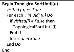
3.11.1 Topological sort ... 43
3.11.2 Single‐source shortest path in a DAG ... 44
Local search ... 45
3.12.1 Neighbourhood function 𝐴𝑠1 ... 46
3.12.2 Neighbourhood function 𝐴𝑠2 ... 46
3.12.3 Neighbourhood function 𝐴𝑠3 ... 46
3.12.4 Neighbourhood function 𝑆𝑒1 ... 46
3.12.5 Neighbourhood function 𝑆𝑒2 ... 46
Summary ... 46
DUAL‐RESOURCE FLEXIBLE JOB‐SHOP SCHEDULING PROBLEM WITH SEQUENCING FLEXIBILITY (DRFJSPS) ... 47
Problem description ... 48
Mathematical formulation ... 48
Illustrative example ... 52
Proposed algorithm ... 54
The elitist non‐dominated sorting GA (NSGA‐II) ... 54
4.5.1 Encoding and decoding of the chromosome ... 57
4.5.2 Initialization of population ... 58
4.5.2.1 Initial parent population assignment ... 58
4.5.2.2 Initial parent population sequencing ... 61
4.5.3.1 Full‐crossover ... 62
4.5.3.2 Resources‐crossover ... 62
4.5.3.3 Sequence‐crossover ... 62
4.5.4 Mutation operator ... 66
4.5.4.1 Resources‐mutation ... 66
4.5.4.2 Sequence ‐mutation ... 66
Summary ... 68
FLEXIBLE JOB‐SHOP SCHEDULING PROBLEM WITH SEQUENCING AND PROCESS PLAN FLEXIBILITY (FJSP‐2F) ... 69
Introduction ... 69
Problem description ... 70
Mathematical formulation ... 71
Illustrative example ... 73
Summary ... 75
APPLICATION IN METAL CUTTING INDUSTRY: CASE STUDY AND DECISION SUPPORT SYSTEM ... 76
Implementation (a decision support system) ... 78
6.1.1 Spreadsheets overview ... 79
Summary ... 83
NUMERICAL EXPERIMENTS ... 84
Design of experiments ... 84
7.1.1 Design of experiments for the HBFOA ... 85
7.1.2 Design of experiments for the NSGA‐II ... 89
Numerical experience for the FJSPS ... 91
Numerical experience for the DRFJSPS ... 101
7.3.2 Comparison of NSGA‐II and the MRSLS ... 105
Numerical experience for the FJSP‐2F ... 141
CONCLUSION ... 148
Research significance ... 148
Limitations... 148
Novelties and contributions ... 148
Future work ... 150
Conclusion ... 150
REFERENCES ... 153
APPENDIX A. INSTANCES ... 158
VITA AUCTORIS ... 193
LIST OF FIGURES
Figure 1.1 Hierarchy of production decisions(adopted from Nahmias (2009)). ... 2
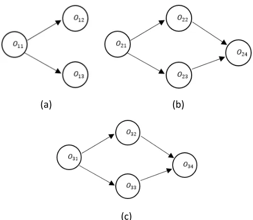
Figure 1.2 Precedence relationship of a single job (a) Sequential order (b) DAG. ... 7
Figure 1.3 Genetic algorithm representation. ... 8
Figure 1.4 Pareto frontier representation for the minimization of two objectives. ... 9
Figure 1.5 Stage 1 for the proposed methodology. ... 12
Figure 1.6 Stage 2 for the proposed methodology. ... 13
Figure 1.7 Stage 3 for the proposed methodology. ... 13
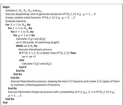
Figure 3.1 BFOA pseudocode. ... 28
Figure 3.2 Hill climbing method. ... 30
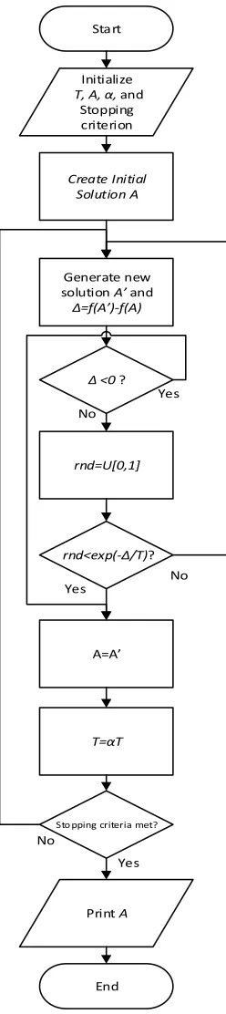
Figure 3.3 Simulated annealing flowchart. ... 31
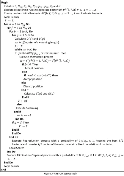
Figure 3.4 HBFOA pseudocode. ... 33
Figure 3.5 Operation precedence for Table 3.1 (a) Job 1; (b) Job 2 ; (c) Job 3. ... 34
Figure 3.6 A feasible solution. ... 34
Figure 3.7 Gantt chart for data of Table 2. ... 34
Figure 3.8 Exchange on OSV swapping 𝑟𝑡ℎ=2 and 𝑠𝑡ℎ=8. ... 37
Figure 3.9 Pseudocode for repair mechanism. ... 38
Figure 3.10 Swarming OSV ( j=3). ... 40
Figure 3.11 Swarming MAV (j=3). ... 40
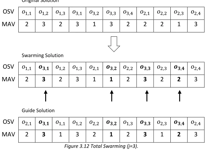
Figure 3.12 Total Swarming (j=3). ... 41
Figure 3.13 Illustration of a disjunctive graph. ... 42
Figure 3.14 Illustration of a DAG. ... 42
Figure 3.15 Illustration of the critical path. ... 43
Figure 3.16 Topological sort algorithm. ... 43
Figure 3.17 TopologicalSortUntil Function. ... 44
Figure 3.18 Single‐source shortest path in DAG. ... 44
Figure 3.19 Local search pseudocode. ... 45
Figure 4.1 Practical the dual job‐shop scheduling model. ... 47
Figure 4.2 Operation precedence for Table 4.1 (a) Job 1; (b) Job 2 ; (c) Job 3. ... 52
Figure 4.3 Machine Gantt chart for illustrative example. Labels per operation (u,j,k). ... 53
Figure 4.4 Worker Gantt chart for illustrative example. Labels per operation (i,u,j,k). ... 54
Figure 4.6 NSGA‐II procedure. ... 55
Figure 4.7 Crowding distance calculation. Adapted from Burke and Kendall (2005). ... 56
Figure 4.8 Crowding distance assignment procedure. ... 56
Figure 4.9 Flowchart of NSGA‐II. ... 57
Figure 4.10 A feasible solution for DRFSPS. ... 57
Figure 4.11 Gantt chart of the decoded feasible solution. ... 58
Figure 4.12 Full‐Crossover example. ... 63
Figure 4.13 Crossover example (resources). ... 64
Figure 4.14 Crossover example (sequence). ... 65
Figure 4.15 Mutation example (resources). ... 66
Figure 4.16 Mutation example (sequence). ... 67
Figure 4.17 Repair mechanism for sequence‐mutation. ... 67
Figure 5.1 Operation precedence. ... 74
Figure 5.2 Gantt chart of the illustrative example. ... 75
Figure 6.1 Operation precedence graphs (Case I, II and III). ... 77
Figure 6.2 DSS Use case diagram. ... 78
Figure 6.3 DSS Structure chart. ... 79
Figure 6.4 DSS Welcome display. ... 80
Figure 6.5 DSS Order input window. ... 80
Figure 6.6 DSS Solution method window. ... 81
Figure 6.7. DSS Results window. ... 82
Figure 6.8 Gantt chart window. ... 82
Figure 6.9 Help display. ... 83
Figure 7.1DOE methodology. ... 85
Figure 7.2 Surface plot of factors ND vs N and t ... 90
Figure 7.3 Gantt chart of machines of DR1‐solution 6. ... 92
Figure 7.4 Gantt chart of machines of DR1‐solution 6. ... 93
Figure 7.5 Gantt chart of machines of DR1‐solution 6. ... 93
Figure 7.6 Gantt chart of Case I. ... 93
Figure 7.7 Gantt chart of Case II. ... 94
Figure 7.8 Gantt chart for Case III. ... 94
Figure 7.10 Gantt chart of BRdata MK07‐MK10. ... 96
Figure 7.11 Gantt chart of problem MK01. ... 97
Figure 7.12 Gantt chart of problem MK02. ... 97
Figure 7.13 Gantt chart of problem (a) MK03; (b) MK04; (c) MK05; (d)MK06. ... 98
Figure 7.14 Gantt chart of problem (a) MK07 and (b) MK08. ... 99
Figure 7.15 Gantt chart of problem (c) MK09 and (d)MK10. ... 100
Figure 7.16 Operation precedence graphs DR1, DR2, DR3, DR4 and DR5. ... 102
Figure 7.17 Flowchart of MRSLS. ... 104
Figure 7.18 Gantt chart of machines of DR1‐solution 1. ... 106
Figure 7.19 Gantt chart of workers of DR1‐solution 1. ... 106
Figure 7.20 Gantt chart of machines of DR1‐solution 2. ... 107
Figure 7.21 Gantt chart of workers of DR1‐solution 2. ... 107
Figure 7.22 Gantt chart of machines of DR1‐solution 3. ... 108
Figure 7.23 Gantt chart of workers of DR1‐solution 3. ... 108
Figure 7.24 Gantt chart of machines of DR1‐solution 4. ... 109
Figure 7.25 Gantt chart of workers of DR1‐solution 4. ... 109
Figure 7.26 Gantt chart of machines of DR1‐solution 5. ... 110
Figure 7.27 Gantt chart of workers of DR1‐solution 5. ... 110
Figure 7.28 Gantt chart of machines of DR1‐solution 6. ... 111
Figure 7.29 Gantt chart of workers of DR1‐solution 6. ... 111
Figure 7.30 Gantt chart of machines of DR1‐solution 7. ... 112
Figure 7.31 Gantt chart of workers of DR1‐solution 7. ... 112
Figure 7.32 Gantt chart of machines of DR2‐solution 1. ... 114
Figure 7.33 Gantt chart of workers of DR2‐solution 1. ... 114
Figure 7.34 Gantt chart of machines of DR2‐solution 2. ... 115
Figure 7.35 Gantt chart of workers of DR2‐solution 2. ... 115
Figure 7.36 Gantt chart of machines of DR3‐solution 1. ... 116
Figure 7.37 Gantt chart of workers of DR3‐solution 1. ... 117
Figure 7.38 Gantt chart of machines of DR3‐solution 2. ... 117
Figure 7.39 Gantt chart of workers of DR3‐solution 2. ... 118
Figure 7.40 Gantt chart of machines of DR3‐solution 3. ... 118
Figure 7.42 Gantt chart of machines of DR3‐solution 4. ... 119
Figure 7.43 Gantt chart of workers of DR3‐solution 4. ... 120
Figure 7.44 Gantt chart of machines of DR3‐solution 5. ... 120
Figure 7.45 Gantt chart of workers of DR3‐solution 5. ... 121
Figure 7.46 Gantt chart of machines of DR3‐solution 6. ... 121
Figure 7.47 Gantt chart of workers of DR3‐solution 6. ... 122
Figure 7.48 Gantt chart of machines of DR3‐solution 7. ... 122
Figure 7.49 Gantt chart of workers of DR3‐solution 7. ... 123
Figure 7.50 Gantt chart of machines of DR3‐solution 8. ... 123
Figure 7.51 Gantt chart of workers of DR3‐solution 8. ... 124
Figure 7.52 Gantt chart of machines of DR3‐solution 9. ... 124
Figure 7.53 Gantt chart of workers of DR3‐solution 9. ... 125
Figure 7.54 Gantt chart of machines of DR4‐solution 1. ... 126
Figure 7.55 Gantt chart of workers of DR4‐solution 1. ... 126
Figure 7.56 Gantt chart of machines of DR4‐solution 2. ... 127
Figure 7.57 Gantt chart of workers of DR4‐solution 2. ... 127
Figure 7.58 Gantt chart of machines of DR4‐solution 3. ... 128
Figure 7.59 Gantt chart of workers of DR4‐solution 3. ... 128
Figure 7.60 Gantt chart of machines of DR4‐solution 4. ... 129
Figure 7.61 Gantt chart of workers of DR4‐solution 4. ... 129
Figure 7.62 Gantt chart of machines of DR4‐solution 5. ... 130
Figure 7.63 Gantt chart of workers of DR4‐solution 5. ... 130
Figure 7.64 Gantt chart of machines of DR4‐solution 6. ... 131
Figure 7.65 Gantt chart of workers of DR4‐solution 6. ... 131
Figure 7.66 Gantt chart of machines of DR4‐solution 7. ... 132
Figure 7.67 Gantt chart of workers of DR4‐solution 7. ... 132
Figure 7.68 Gantt chart of machines of DR4‐solution 8. ... 133
Figure 7.69 Gantt chart of workers of DR4‐solution 8. ... 133
Figure 7.70 Gantt chart of machines of DR4‐solution 9. ... 134
Figure 7.71 Gantt chart of workers of DR4‐solution 9. ... 134
Figure 7.72 Gantt chart of machines of DR5‐solution 1. ... 135
Figure 7.74 Gantt chart of machines of DR5‐solution 2. ... 136
Figure 7.75 Gantt chart of workers of DR5‐solution 2. ... 137
Figure 7.76 Gantt chart of machines of DR5‐solution 3. ... 137
Figure 7.77 Gantt chart of workers of DR5‐solution 3. ... 138
Figure 7.78 Gantt chart of machines of DR5‐solution 4. ... 138
Figure 7.79 Gantt chart of workers of DR5‐solution 4. ... 139
Figure 7.80 Gantt chart of machines of DR5‐solution 5. ... 139
Figure 7.81 Gantt chart of workers of DR5‐solution 5. ... 140
Figure 7.82 Gantt chart of machines of DR5‐solution 6. ... 140
Figure 7.83 Gantt chart of workers of DR5‐solution 6. ... 141
Figure 7.84 Operation precedence graphs. ... 142
Figure 7.85 Operation precedence graphs continued. ... 143
Figure 7.86 Gantt chart of solution 1. ... 145
Figure 7.87 Gantt chart of solution 2. ... 146
Figure 7.88 Gantt chart of solution 3. ... 146
Figure 7.89 Gantt chart of solution 4. ... 147
Figure 8.1 Novelties and contributions. ... 149
LIST OF TABLES
Table 2.1 Synthesis matrix. ... 21
Table 3.1 Data of instance of 3 jobs and three machines. ... 32
Table 3.2 Initial machine assignment by AssigmentRule3 (machine workload updates in bold).. 35
Table 4.1 Data of an illustrative instance. ... 53
Table 4.2 Objective values for the illustrative example. ... 53
Table 4.3 Initial machine assignment by AssigmentRule4 (1) (machine workload updates in bold). ... 59
Table 4.4 Initial machine assignment by AssigmentRule4 (2) (machine workload updates in bold). ... 59
Table 4.5 Initial machine assignment by AssigmentRule4 (3) (machine workload updates in bold). ... 60
Table 4.6 Initial machine assignment by AssigmentRule5 (1) (machine workload updates in bold). ... 60
Table 4.7 Initial machine assignment by AssigmentRule5 (2) (machine workload updates in bold). ... 61
Table 4.8 Initial machine assignment by AssigmentRule5 (3) (machine workload updates in bold). ... 61
Table 5.1 Processing times and cost of an illustrative instance. ... 73
Table 5.2 The experimental results for the weighted tardiness data. ... 74
Table 6.1 Case I Operation precedence graph. ... 77
Table 6.2 Case II Operation precedence graph. ... 78
Table 6.3 Case III Operation precedence graph. ... 78
Table 7.1 Parameter levels for the HBFOA. ... 86
Table 7.2 Analysis of variance output from Minitab for the makespan. ... 87
Table 7.3 Significant factors of HBFOA for the makespan. ... 87
Table 7.4 Analysis of variance output from Minitab for the weighted tardiness. ... 88
Table 7.5 Significant factors of HBFOA for the weighted tardiness. ... 89
Table 7.6 Parameter levels for the NSGA‐II. ... 89
Table 7.7 Analysis of variance output from Minitab for the multi‐objective problem. ... 90
Table 7.8 Setting for the significant factors of NSGA‐II for the multi‐objective problem. ... 90
Table 7.10 The experimental results for the BRdata. ... 94
Table 7.11 Instances for the (DRFJSPS). ... 101
Table 7.12 DR1 operation precedence graph. ... 103
Table 7.13 DR2 operation precedence graph. ... 103
Table 7.14 DR3 operation precedence graph. ... 103
Table 7.15 DR4 operation precedence graph. ... 103
Table 7.16 DR5 operation precedence graph. ... 103
Table 7.17 Comparison of the NSGA‐II and the MRSLS (DR1). ... 105
Table 7.18 Comparison of the NSGA‐II and the MRSLS (DR2). ... 113
Table 7.19 Comparison of the NSGA‐II and the MRSLS (DR3). ... 116
Table 7.20 Comparison of the NSGA‐II and the MRSLS (DR4). ... 125
Table 7.21 Comparison of the NSGA‐II and the MRSLS (DR5). ... 135
Table 7.22 Percentage of contribution to the non‐dominated set. ... 141
Table 7.23 Parameter for instances PP1, PP2 and PP3. ... 142
Table 7.24 Operation precedence graph PP1. ... 143
Table 7.25 Operation precedence graph PP2. ... 144
Table 7.26 Operation precedence graph PP1. ... 144
Table 7.27 PP1 Experimental results for FJSP‐2F. ... 145
Table 7.28 PP2 Experimental results for FJSP‐2F. ... 147
Table 7.29 PP3 Experimental results for FJSP‐2F. ... 147
Table A.1 Case I 10 x 15 with 63 operations. ... 158
Table A.2 Case I 10 x 15 with 63 operations (continued). ... 159
Table A.3 Case II 5 x 12 with 25 operations. ... 159
Table A.4 Case III 8 x 14 with 44 operations. ... 160
Table A.5 DR1 10 x 15 x 10 with 63 operations. ... 161
Table A.6 DR1 10 x 15 x 10 with 63 operations (continued). ... 162
Table A.7 DR1 10 x 15 x 10 with 63 operations (continued). ... 163
Table A.8 DR1 10 x 15 x 10 with 63 operations (continued). ... 164
Table A.9 DR1 10 x 15 x 10 with 63 operations (continued). ... 165
Table A.10 DR1 10 x 15 x 10 with 63 operations (continued). ... 166
Table A.11 DR1 10 x 15 x 10 with 63 operations (continued). ... 167
Table A.13 DR1 10 x 15 x 10 with 63 operations (continued). ... 169
Table A.14 DR1 10 x 15 x 10 with 63 operations (continued). ... 170
Table A.15 DR1 due dates and weights. ... 171
Table A.16 DR2 5 x 12 x 3 with 25 operations. ... 171
Table A.17 DR2 5 x 12 x 3 with 25 operations (continued). ... 172
Table A.18 DR2 due dates and weights. ... 172
Table A.19 DR3 8 x 13 x 4 with 44 operations. ... 173
Table A.20 DR3 8 x 13 x 4 with 44 operations (continued). ... 174
Table A.21 DR3 8 x 13 x 4 with 44 operations (continued). ... 175
Table A.22 DR3 8 x 13 x 4 with 44 operations (continued). ... 176
Table A.23 DR3 due dates and weights. ... 176
Table A.24 DR4 6 x 6 x 3 with 41 operations. ... 177
Table A.25 DR4 due dates and weights. ... 177
Table A.26 DR5 7 x 8 x 5 with 47 operations. ... 178
Table A.27 DR5 7 x 8 x 5 with 47 operations (continued). ... 179
Table A.28 DR5 due dates and weights. ... 180
Table A.29 Due dates and weights FJSP‐2F instance PP1. ... 180
Table A.30 PP1 FJSP‐2F instance 10 x 5 with 146 operations. ... 181
Table A.31 PP1 FJSP‐2F instance 10 x 5 with 146 operations (continued). ... 182
Table A.32 PP1 Costs FJSP‐2F instance 10 x 5 with 146 operations. ... 183
Table A.33 PP1 Costs FJSP‐2F instance 10 x 5 with 146 operations (continued). ... 184
Table A.34 PP2 FJSP‐2F instance 5 x 8 with 70 operations. ... 185
Table A.35 PP2 FJSP‐2F instance 5 x 8 with 70 operations (continued). ... 186
Table A.36 Due dates and weights FJSP‐2F instance PP2. ... 186
Table A.37 Costs PP2 FJSP‐2F instance 5 x 8 with 70 operations. ... 187
Table A.38 Costs PP2 FJSP‐2F instance 5 x 8 with 70 operations (continued). ... 188
Table A.39 PP3 FJSP‐2F instance 6 x 6 with 111 operations. ... 188
Table A.40 PP3 FJSP‐2F instance 6 x 6 with 111 operations (continued). ... 189
Table A.41 PP3 FJSP‐2F instance 6 x 6 with 111 operations (continued). ... 190
Table A.42 Due dates and weights PP3 FJSP‐2F instance. ... 190
Table A.43 Costs PP3 FJSP‐2F instance 6 x 6 with 111 operations. ... 190
Table A.45 Costs PP3 FJSP‐2F instance 6 x 6 with 111 operations (continued). ... 192
LIST OF ABBREVIATIONS
ACO Ant Colony Optimization
ANOVA Analysis of Variance
BFOA Bacterial Foraging Optimization Algorithm
DAG Directed Acyclic Graph
DOE Design of Experiments
DSS Decision Support System
DRFJSPS Dual‐Resource Flexible Job Shop with Sequencing flexibility
EA Evolutionary Algorithm
FJSP Flexible Job Shop Scheduling Problem
FJSPS Flexible Job Shop Scheduling Problem with Sequencing flexibility
FJSP‐2F Flexible Job Shop Scheduling Problem with sequencing and process plans
Flexibility
FMS Flexible Manufacturing System
GA Genetic Algorithm
HA Hybrid Algorithms
HBFOA Hybrid Bacterial Foraging Optimization Algorithm
JSP Job‐shop Scheduling Problem
LEGA LEarnable Genetic Architecture
MAV Machine Assignment Vector
MILP Mixed Integer Linear Programming
MOEA Multi‐objective Evolutionary Algorithm
MRP Material Requirement Planning
MRSLS Multi Random Search
NRGA Non‐dominated Ranking Genetic Algorithm
NSGA‐II Elitist Non‐dominated Sorting Genetic Algorithm
OSV Operation Sequence Vector
SA Simulated Annealing
SI Swarm Intelligence
SME Small Medium Enterprise
SPS Single Point Search
TS Tabu Search
VBA Visual Basic for Applications
INTRODUCTION
In this chapter, the motivation of this research is presented. Then, a brief overview of the
production scheduling problem and how to tackle is provided. Machine scheduling under the
bigger umbrella of production planning is outlined. Scheduling terminology is presented, and the
base of the scheduling function importance is discussed. Moreover, an introduction to
evolutionary algorithms and multi‐objective optimization is given. Finally, the objectives and
research plan of this research are being presented.
Motivation
Marketing strategists usually advocate increased product variety in order to attend better
to market demand. Furthermore, companies often acquire more advanced
manufacturing systems to take care of the increased product mix and unpredictable
demand. Flexible manufacturing systems (FMS) is an example of the production
environment that has been used to answer the needs of a turbulent market environment.
This production system encompasses different levels of changeability. They have been
implemented but are not fully optimized. Strategic scheduling of these complex systems
would thus require decisions with conflicting objectives. Hence, methodologies to tackle
these problems would be needed to foster a thriving industry.
The FJSP is an extension of the classical job‐shop scheduling problem (JSP), where
operations can be performed by a set of candidate capable machines (Brandimarte 1993).
Process planning is a significant function in the manufacturing process, and this is the
process of selecting and sequencing manufacturing processes by achieving one or more
objectives (Shen
et al.
2006). A process plan is generated without information of the
current manufacturing resources, and it lacks consideration of scheduling objectives. The
process plan created could also not be feasible due to the present manufacturing
scenario. Generally, some modifications of the process plan need to be done to reflect
the updated shop floor status. Sequential executions of the process planning and
that take into account the objectives that both problems could optimize should be
considered.
Production scheduling
The process to arrange a set of task over the time where capability, capacity and time constraints
are considered is defined as the production scheduling problem (Lopez and Roubellat 2013).
Production scheduling can be seen as a decision‐making process that is used on a regular basis in
many manufacturing and service industries (Pinedo 2005). In order to describe the importance of
scheduling process, it is necessary to show how it fits under the bigger picture of the production
function.
Production scheduling is a crucial element of the production function. The production function
can be view as a hierarchical process (Nahmias 2009). The first step is to forecast the demand for
aggregate sales. The forecast should be done over a predefined planning horizon. These data are
the input to create an aggregate plan (aggregate production and workforce levels) which will be
translated into the master production schedule (MPS). The MPS results in specific production
goals by product and time period.
One technique to reach the production goals of finished‐goods inventory produced by the MPS is
the materials requirement planning (MRP). The MRP breaks down the MPS into a detailed
schedule of production of each component that comprises an end item. The result of the MRP is
transformed into specific shop floor schedules that include a set of tasks and due dates related to
those tasks. An illustration of this hierarchical process can be found in Figure 1.1.
Production scheduling is one of the critical production planning enablers to facilitate
responsiveness and agility to achieve such flexibility. In many productions systems the scheduling
function is usually performed by first line management, but over the years this function has
become a more complex task to achieve. For this reason, much attention has been brought to the
scheduling function.
The traditional job‐shop scheduling problem (JSP) is defined as the suitable sequencing of a set of
jobs that must be processed on different machines while satisfying a set of prescribed precedence
constraints (Demir and Kürşat İşleyen 2013). The job‐shop scheduling problem has been widely
studied since the 1950s (Özgüven et al. 2010). JSP has been proved to be NP‐hard (Garey et al.
1976).
This research work, review the different techniques that have been proposed over the years and
establish a methodology to study an extension of the FJSP.
Scheduling framework
In scheduling theory, the number of jobs and machines are assumed to be finite. 𝑛 represents the number of jobs and the number of machines is define by 𝑚. Generally, the index 𝑗 is used to refer to a job and the index 𝑖 is employed to denote a machine. The processing of a job 𝐽 on machine
𝑀 is called an operation 𝑜 .
Scheduling problems are usually described by a triplet 𝛼 | 𝛽 | 𝛾 (Pinedo 2005). The first entry 𝛼 represents the machine environment. The second entry 𝛽 provides information of processing characteristics and constraints. It might comprise no entry at all or multiple entries. The last entry
𝛾 describes the objective to be minimized.
The most basic machine environments 𝛼 are described by Pinedo (2005) as follows:
Parallel machines (Pm): There are m identical machines in parallel. Each job needs one and only one of these machines.
Flow shop (Fm): All the jobs have to be processed on each one of the machines, and each job has to follow the same route.
processed first at Stage 1, then Stage 2, and so on. A stage functions as a bank of parallel
machines; at each stage, job 𝑗 requires processing on only one machine and any machine can perform the job.
Job shop (Jm): In this case, each job has its own predefined route to follow through the machines.
Flexible job shop (FJc): A flexible job shop is a generalization and the parallel machine environment. Each job has its own route to follow through the shop. Each job is processed
only by specific machines.
Open shop (Om): Each job has to be processed on each machine. However, some of these processing time may be zero. There are no restrictions with regard to the routing of each
job through the machine environment. The scheduler is allowed to determine a route for
each job, and different jobs may have different routes.
The typical processing restrictions and constraints in the second entry 𝛽 are provides as follow:
Sequence‐dependent setup times (𝑠 ): The 𝑠 represents the sequence dependent setup time between jobs 𝑗 and 𝑘.
Precedence constraints (prec): In this case, one or more jobs need to be completed before another job is allowed to start its processing.
Machine eligibility restrictions (𝑀): In this scenario, some of the machine are capable of processing job 𝑗. 𝑀 symbolizes a set of capable machines that can process the job 𝑗. For the last entry 𝛾, the most common objectives used are:
Makespan (𝐶 ): Completion time of the last job on the system.
Maximum lateness (𝐿 ): The lateness of a job is define by 𝐿 𝐶 𝑑. 𝐶 represents the completion time of job 𝑗 and 𝑑 is the due date of a job. 𝐿 0 when a job is completed late and 𝐿 0 when is completed early. The 𝐿 measures the worst violations of the due dates.
Flexibility in manufacturing systems
Review of the literature identifies at least ten types of manufacturing systems flexibilities
(ElMaraghy 2005). These are:
1. Machine flexibility: Various operations performed without set‐up change,
2. Material handling flexibility: Number of used paths / total number of possible paths
between all machines,
3. Operation Flexibility: Number of different processing plans available for part fabrication,
4. Process Flexibility: Set of part types that can be produced without major set‐up changes,
i.e. part‐mix flexibility,
5. Product Flexibility: Ease (time and cost) of introducing products into an existing product
mix. It contributes to agility,
6. Routing Flexibility: Number of feasible routes of all part types/Number of part types,
7. Volume Flexibility: The ability to vary production volume profitably within production
capacity,
8. Expansion Flexibility: Ease (effort and cost) of augmenting capacity and/or capability,
when needed, through physical changes to the system,
9. Control Program Flexibility: The ability of a system to run virtually uninterrupted (e.g.
during the second and third shifts) due to the availability of intelligent machine and
system control software,
10. Production Flexibility: Number of all part types that can be produced without adding
major capital equipment.
Introduction to the flexible job‐shop problem
The manufacturing companies, in an effort to react to the unpredictable demand, acquire more
manufacturing equipment. The new machines usually have more advanced capabilities. For
instance, the new equipment may process operations faster, and it could handle larger capacities.
Generally, companies maintain the two kinds of manufacturing resources. In this manner, in case
of a breakdown or scheduled maintenance, the old resource can be used to keep the production
running. Furthermore, the old resource can be used as a method to balance the production when
new and old equipment. These new production environments are a new challenge for managers
when they have to execute the production function.
In response to the new productions environments, an extension of the JSP named flexible job
shop scheduling problem (FJSP) has been developed. The FJSP was first presented by Brucker and
Schlie (1990), it allows operations to be processed on any of the available flexible machines, the
machines are not necessarily identical. The flexibility in an FJSP can be either total or partial
(Kacem et al. 2002b). Total flexibility is defined when all the operations can be processed on any
of the machines, and partial flexibility is when some operations can be processed on the available
machines.
The decision involved in the FJSP can be categorized into sub‐problems (Brandimarte 1993):
Routing sub‐problem: The assignment of each operation to a machine out of a set of capable machines is performed.
Scheduling sub‐problem: It is as well known as the sequencing problem. This type of problem selects the operation sequence of all the jobs.
Pinedo (2005) represents a FJSP with total flexibility with 𝐹𝐽𝑐|𝐶 and the case of partial flexibility 𝐹𝐽𝑐|𝑀 |𝐶 . The FJSP belongs to the NP‐hard class (Demir and Kürşat İşleyen 2013). Due to the intractable complexity of the FJSP, two elementary approaches have been developed
(Brandimarte 1993):
Concurrent approach: The general idea of this approach is to tackle the routing and scheduling problem together. In other words, the problems are integrated.
Hierarchical approach: This approach has been widely used, and it explodes the main problem, and it handles each problem (routing and scheduling) in a sequential manner.
1.5.1
Sequencing flexibility
The FJSP assumes sequential order precedence relationships. For some production environments,
the precedence relationship between the operations is not always given in a sequential order. It
can be determined by a directed acyclic graph (DAG). This situation is illustrated in Figure 1.2. The
decisions involved in this extension of the FJSP, consist of the machine assignment and the
assurance of the precedence constraints. Hence, the FJSP with sequencing flexibility permits the
(Birgin et al. 2015). This research considers the mentioned extension, that is a typical example in
industries such as printing (Birgin et al. 2015; Birgin et al. 2014; Vilcot and Billaut 2008), glass
(Alvarez‐Valdés et al. 2005), mould (Gan and Lee 2002) and the cutting tool industry. For instance,
in the cutting tool industry, the FJSP with sequencing flexibility is tackled. Specifically, during the
honing and heat treat operations. The execution of these two operations does not present a
relationship. That is, honing could be performed after or before heat treat without any problem
in the production process. Nevertheless, this sequence flexibility gives the advantage to managing
the production resources better. The manager could decide on the process to be performed based
on the machines’ availability.
(a)
(b)
Figure 1.2 Precedence relationship of a single job (a) Sequential order (b) DAG.
Evolutionary algorithms
Metaheuristics based on natural selection are known as Evolutionary Algorithms (EA). These
solution methods are based on a population of solutions that are generated, selected, combined
and updated. There are three types of EA: Genetic algorithms (GA), Evolutionary programming
(EP) and Evolutionary Strategies (ES). EAs have proven very successful in practical applications,
they are highly flexible and can be configured to address any optimization task. EA uses three
evolutionary operators (mutation, recombination and selection) to generate better solutions.
Mutation and recombination are used to create a new solution. Then, above‐average individuals
in the population are selected (reproduced) to become members of the next generation (Coello
et al. 2007).
1.6.1
Genetic algorithms
GA are search methods based on principles of natural selection and genetics. GA have been widely
used to generate high‐quality solutions to optimization problems. This algorithm reflects the
process of natural selection where the fittest individuals are selected for reproduction in order to
GA encode the decision variables of a problem in a chromosomal manner and use a fitness
measure for discriminating good solutions from bad ones. GA is initialized with a set of random
solutions called population. Each solution in the set is named a chromosome that represents a
problem solution. The chromosomes are evaluated with a fitness function to determine how well
the solutions solve the problem. This function is used to select parents that are used to create
new generations. Two processes are employed for the formation of a new solution, usually called
offspring. The first process is the crossover or recombination, with the selected characteristics
from the parents creates a new solution. The second process is the mutation in which new genetic
material is introduced. After the mutation process, the solutions are evaluated with the fitness
function. The top scoring members of the population are chosen. The algorithm continues running
up to it reaches a specified number of runs or a fitness threshold. After several generations, the
algorithm converges to the best solution (Burke and Kendall 2005).
Figure 1.3 Genetic algorithm representation.
Multi‐objective optimization
Decision making usually involves conflicting objectives. In real problems, no single solution
simultaneously optimize those conflicting objectives. Contrary, there is a set of trade‐off optimal
solutions, so the user would be in a better position to make a choice when many such trade‐off
solutions are unveiled (Burke and Kendall 2005).
For multi‐objective optimization, multiple fitness functions are used to provide a set of optimal
solutions. This set of solutions contains elements that are equally optimal as none of the objective
functions can be improved in value without degrading some of the other objective values. That
is, no solution dominates any other solution in the frontier as presented in Figure 1.4. These
solutions are usually called non‐dominated solutions or Pareto‐optimal solutions. Several
methods for multi‐objective optimization have been developed in the literature, from the classic
methods as the weighted‐ sum approach and 𝝐‐constraint method to the elaborated evolutionary algorithms (Burke and Kendall 2005).
Figure 1.4 Pareto frontier representation for the minimization of two objectives.
1.7.1
Weighted‐sum approach to multi‐objective optimization
The simplest method for multi‐objective optimization is the weighted‐sum approach. This method
reflect the decision maker’s preference. As the determination of specific values of those weights
is subjective, this method could yield only an efficient but not optimum solution. Additionally, the
weight vector corresponds to a pre‐destinated optimal solution on the Pareto frontier. Hence,
changing the weight vector, a different Pareto‐optimal point can be obtained (Burke and Kendall
2005).
1.7.2
Elitist non‐dominated sorting GA (NSGA‐II)
Multi‐objective evolutionary algorithms (MOEAs) have been used in the literature due to their
ability to find multiple Pareto‐optimal solutions in one single simulation run (Deb et al. 2002). The
nondominated sorting genetic algorithm (NSGA) was proposed by (Srinivas and Deb 1994). This
algorithm has been criticized due to its high computational complexity, the lack of elitism
approach and the need for specifying a sharing parameter (Deb et al. 2000). Hence, to solve the
algorithms pitfalls, the elitist non‐dominated sorting GA (NSGA‐II) was introduced by Deb et al.
(2002).
The NSGA‐II for multiple Pareto‐optimal solutions in a multi‐objective optimization has three
essential features: It uses an elitist principle, it uses an explicit diversity preserving mechanism,
and it emphasizes the non‐dominated solutions (Burke and Kendall 2005). NSGA‐II tends to spread
quickly and appropriately when a certain non‐dominated region is found.
Thesis statement
The integration of dual‐resource approach, sequencing flexibility, process plan flexibility and
process plan cost for the FJSP and the development of mathematical models and new
metaheuristics yields a better scheduling solution that requires less time and cost.
Mathematical programming and metaheuristics, specifically the hybrid bacterial foraging
optimization algorithm and Elitist Non‐dominated Sorting GA, can solve the FJSP efficiently with
sequencing flexibility.
Research objectives
The overall objectives of the proposed work are as follow:
2. Develop and implement a metaheuristic to solve larger instances of the extended version
of the FJSP.
3. Formulate a mathematical model for the dual‐resource FJSP with sequencing flexibility.
4. Develop and implement a metaheuristic to solve larger instances of the dual‐resource
FJSP with sequencing flexibility.
5. Develop a mathematical model for the FJSP with sequencing and process plan flexibility
and incorporate the processing cost.
6. Provide instances with these features to the literature.
Research plan
The proposed methodology is comprised of three stages. The first one is called “A MILP
formulation for the FJSP with sequencing flexibility.“ The second one is named “A mathematical
model and metaheuristic for the dual‐resource FJSP with sequencing flexibility.” The third stage
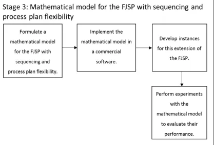
is entitled “Mathematical model for the FJSP with sequencing and process plan flexibility,” which
is to be started after finish the second stage. The steps for each stage are shown in Figure 1.5,
Figure 1.6 and Figure 1.7, respectively.
The first step of Stage 1 develops a single objective mathematical model. The model will
incorporate the sequencing flexibility condition. An MILP formulation technique that minimizes
the weighted tardiness or makespan will be used. The mathematical formulation is a crucial step
to understand the structure of the problem and to develop an effective metaheuristic (Unlu and
Mason 2010). The next step is related to the metaheuristic implementation. A search will be done
for a proper metaheuristic that can be used as an alternative for the most popular metaheuristics.
Special attention has to be taken to find a metaheuristic that takes into account the different
characteristics of the FJSP. Most of the metaheuristics employ parameters that need to be set
based on the problem nature. A technique that can be used to set these parameters is design of
experiments, specifically a 2 factorial design. The 2 factorial design is suitable in factor screening process (Montgomery 2008). This design works with the smallest number of runs where
k factors can be studied. This technique has been used for several authors to set up metaheuristics
parameters, an example is provided in Vital Soto et al. (2017). This type of design will be helpful
to detect the significant main factors and interactions. After this, a regression model can be
generated to find the parameter settings (main factor and/or interactions) that yield the best
surface methodology, in case of the need of more specific parameters values. The last two steps
of stage 1 are based on the efficiency evaluation of the mathematical model against alternative
formulations and to perform experiments with well‐known instances for FJSP.
For stage 2, the same methodology explained for stage 1 will be carried out with the addition of
the development of instances with worker selection. Some of the instances will be taken from the
literature and modified to suit the current problem. The mathematical formulations will take into
account a multi‐objective optimization with objective functions that can capture current
manufacturing environments as minimization of the weighted tardiness, maximal worker
workload and makespan.
For stage 3, a new mathematical formulation will be developed to consider process plan and
sequencing flexibility. The multi‐objective will study the minimization of processing cost,
makespan and weighted tardiness. Several instances will be created to test the performance of
the mathematical formulation.
Figure 1.5 Stage 1 for the proposed methodology.
Figure 1.6 Stage 2 for the proposed methodology.
Figure 1.7 Stage 3 for the proposed methodology.
LITERATURE REVIEW
The FJSP has been studied during the last 28 years. This chapter provides the most relevant
literature for the FJSP. It emphasizes to classify the researched performed in two categories:
mathematical formulations and metaheuristics. Then, this review identifies gaps in the literature
that lead to the formulation of this research.
Mathematical formulations for the flexible job‐shop scheduling problem
Mathematical models for production scheduling were first developed around 1960 (Özgüven et
al. 2010). Wagner (1959), Manne (1960) and Bowman (1959) presented mathematical
formulations that categorized the different mathematical formulation. These categories are
identified as position‐based, sequence‐based and time‐based.
2.1.1
Position‐based model
Wagner (1959) proposed the first position based mathematical model for the JSP. The base of this
formulation assumes that each machine has some positions or slots. This approach considers a
binary variable that assigns an operation to a position on a machine. For the FJSP, Lee et al. (2002)
were the first to introduce a mathematical formulation to minimize makespan considering
process plan flexibility, outsourcing, and due dates. Later, Fattahi et al. (2007) presented a mixed
integer linear programming (MILP) to minimize makespan and testing problems (small and
medium‐large size problems). With their formulation, they were able to solve small size problems
and for medium‐large size problem upper and lower bounds were reported. Similarly, Fattahi et
al. (2009) proposed an MILP allowing overlapping in operation when minimizing makespan. The
authors presented the situation where each job has a demand for more than one, a case usual in
petrochemical industries.
Roshanaei et al. (2013) studied two MILP models for the FJSP. Minimization of makespan was
selected as the optimization criterion. They analyzed their models by examining data proposed
by Fattahi et al. (2007), and they studied an industrial problem in a mould and die‐making shop
as well. The performance of their model was assessed by counting the binary, continuous
as size complexity, computational time and the quality of schedules generated. Their position
based model outperformed the mathematical formulation presented by Fattahi et al. (2007)
based on the performance measures proposed.
Abdi Khalife et al. (2010) developed a multi‐objective FJSP with overlapping in operations. In their
study, they considered a multi‐objective function that comprises makespan, critical machine work
loading time, and total machine work loading time.
2.1.2
Sequence‐based model
Manne (1960) was the pioneer to propose a sequence based mathematical model for JSP. The
model bases his functionality by precedence binary variables that define a sequence of operations
that are assigned to the same machine. Disjunctive Constraints are presented in this formulation.
For the FJSP, Kim and Egbelu (1999) developed an MILP model involving multiple process plan.
The model determines both process plan and a schedule that minimize makespan. Another
essential mathematical formulation is the one studied by Low and Wu (2001). They proposed a 0‐
1 integer programming model with the objective of minimizing the total tardiness in a flexible
manufacturing system considering setup time. The setups were assumed to be sequence
independent. They presented a linearization of their quadratic constraints.
Zhang et al. (2012) showed a model for the FMS with transportation and bounded processing time
to minimize makespan and storage. In this study, all jobs need to be transported to be processed
by a machine, the transportation can be done by any transport and the loading/unloading time is
machine dependent.
Özgüven et al. (2010) established two MILP models. The first model deals with FJSP minimizing
makespan, and it is compared with the model presented by Fattahi et al. (2007). The second
model studied the FJSP by adding process plan flexibility.
Other considerations have been formulated for the FJSP, Gao, Gen, et al. (2006) modelled a
situation when the availability of the machines is compromised due to maintenance, pre‐
schedules, etc. The authors studied the FJSP with non‐fixed availability constraints. In this study,
the model minimizes three objectives defined as makespan, maximal machine workload and total