Implementation of Dynamic Programing to Find All Pairs Shortest Path on Fibre Optics Networks to Produced Optimized Routing and Virtual Topology

(1)

Implementation of Dynamic Programing to Find All

Pairs Shortest Path on Fibre Optics Networks to

Produced Optimized Routing and Virtual Topology

A.Ravi Chandra Reddy

1

, Dr.V.Raghunatha Reddy

2

Research Scholar, Department of Computer Science & Technology, Sri Krishnadevaraya, Anantapur, India1

Assistant Professor, Department of Computer Science &Technology, Sri Krishnadevaraya,Anantapur, India2

ABSTRACT: Optical fibre has been the main choice of communication medium for long-haul networks because of its low transmission loss and high capacity of the data rate. A fibre cable can transmit many channels simultaneously using wavelength Division multiplexing (WDM) technology. This makes possible to establish many different virtual topologies on top of the physical topology. In this paper, dynamic programming model has been developed to produce different sets of traffic matrices for finding shortest path from each source to different destinations. On which existing Heuristic logical design Algorithm (HLDA) is implemented to find shortest path by varying number of optical transceivers. A study is made on stage wise 4-node, 7-node and 14-node NSFNET traffic matrices and comparative study has been done on utilisation of Average Weighted hops and Wavelength.

KEYWORDS: Fibre Optics, Dynamic programming, Virtual Topology, All pair shortest path, Stages, Minimum Congestion, Maximum Congestion.

I.INTRODUCTION

Optical networks using wavelength-division multiplexing (WDM) is seen as the technology of the future. With explosive growth of Internet and bandwidth-intensive applications such as video-on-demand and multimedia, conferencing the demand for bandwidth at lower costs is increasing every day. As such, a ration of research has been carried out in this area. A WDM optical network consists of wavelength routing nodes interconnected by point-to- point optical ﬁbre links in a random topology. The WDM is a multiplexing technique that has led to efficient bandwidth utilizations up to few Tb/s. It is a method of transmitting data simultaneously at multiple carrier wavelengths over a ﬁbre such that they do not interfere with each other

(2)

The virtual topology design problem can be formulated as a mixed-integer linear programming (MILP) problem [4] [Rama swami et al., 1996, and 1998]. It resembles the multi commodity flow problem, where a commodity corresponds to a light path and flow on an edge corresponds to traffic flow offered onto the edge. The objective is to design a virtual topology to optimize a certain metric subject to a set of constraints. The problem has been formulated as an optimization problem by [5] Mukherjee, Banerjee, Ramamurthy and Mukherjee [Mukherjee et al., 1996]. Some possible objective functions to minimize congestion, minimize average weighted hop count.

[6] [Banerjee et al., 2000], maximizing single hop traffic and minimizing message delay. Being an NP-hard problem, the virtual topology design is computationally intractable. It becomes almost impractical to solve when the network size becomes larger. Therefore, there is a need for good heuristic solutions that give reasonably good results close to the optimum one. A number of heuristic algorithms are given in the literature [Banerjee et al., 2000; Ozdaglar et al., 2003]. [7]Ghose, Kumar, Banerjee and Dutta [Ghose et al., 2005] compared the queuing delay in an optical network using both Poisson and self-similar traﬃc. They showed that the virtual topologies designed using self-similar traffic are more effective in handling present day brusty Internet traffic. In the static case the traffic in the network is known a priori with the help of a traffic matrix. The source-destination pair for setting up light path can be chosen in a particular order to establish an eﬃcient virtual topology with the limited number of available wavelengths. Researchers have given various schemes to line up the connection requests while setting up the light paths for the static virtual topology [Chlamtac et al., 1992, 1996; Zhang et al., 1995; Ram swami et al., 1996]. The performances of these existing policies heavily depend upon the physical topology of the networks.

Dynamic programming is an inductive design technique, similar to ‗greedy approach‘ and ‗divide and conquer‘. Dynamic programming divides a problem into a set of sub problems and founds a recursive relationship among the original problem and its sub problems. A sub problem that represents a small part of the original problem is solved for obtaining the optimal solution. Then the scope of this sub problem is enlarged to find the optimal solution of a new sub problem. This process of enlargement is repeated till the scope of the sub problem involves the whole original problem. Thereafter, solution for the whole problem is obtained by combining the optimal solutions of its sub problems.

II.RELATED WORK

Finding shortest paths is an important and fundamental problem in communication network and transportation networks, circuit design, graph analysis Internet node traﬃc, social networking, and graph analysis [8] (Girvan & New- man, 2002)—and is a sub-problem of many combinatorial problems, such as those that can be represented as a network ﬂow problem The heuristic logical topology design algorithm (HLDA) is the main objective is to minimize the congestion in the congestion in the network.it efforts to control set of light paths in terms of their source and destination nodes .in given network the traffic matrix and physical topology are taken as the input and stage wise we can find out all pair shortest path.

[9] In a multistage graph G = <V, C> for given physical topology is taken is a directed graph where the vertices (nodes) are partitioned into k ≥ 2, disjoint sets Vi, where 1 ≤ i ≤ n. Every edge (links) connects two nodes from

two partitions. Each edge is associated with an edge cost C (i, j). The initial node is called a source and the last node is called a sink. The multistage problem is a problem of finding the shortest path from the source to the destination. This problem is also called the ‗stage coach problem‘. The dynamic programming approach can be used to solve this problem

Given a directed graph G =(V,E) with n vertices V = {v1,v2,...,v n}and m edges E = {e1,e2,...,e m},the distance version of the algorithm work out the length of the shortest path from vi to v j for all (vi, v j) pairs. The full version also returns the actual paths in the form of an ancestor matrix.

III.SCOPE OF RESEARCH

(3)

Stages: The given traffic matrix based on physical topology on the length of each node we can divide into number of sub problems, called stages.

Decision: In every stage, there can be multiple decisions out of which the best shortest path (least cost)

State: A state indicates the stages for which decision needs to be taken. The variables that are used to take a decision at every stage are called state variables.

Policy: A policy is a rule that determines the decision at each stage. A policy is called an optimal policy if it is globally optimal.

Principle of Optimality: It states that the optimal sequence of decisions in a multistage decision problem is feasible if and only if its sub-sequences are optimal.

The uses the dynamic programming approaches for finding the shortest path between any two given two nodes. The input for the algorithm is a network G = <V, E>, and a set of weights w I jfor each (i, j) ∈E. algorithm finds the

shortest simple path from node s to node t. The input for the algorithm is an adjacency matrix of the graph G. The cost (i, j) is computed as follows

Initially, the matrix D (0) is initialized as cost (i, j). Then, in subsequent iterations, the next matrix D is computed. Now D (1) is computed with only one intermediate node {1}. D (2) is computed with only two intermediate nodes {1, 2}. In general, D (k) is computed from D (k−1) and there are only two possibilities for computing it, which

are as follows:

1. The first possibility is that node k is not involved. Since the node is not part of the path, only nodes {1, 2, tok

− 1} are considered. Hence, Dij(k) = Dij(k−1).

2. The second possibility is that node k is used as an intermediate node. In this case, one Can split the path as I->k and k+1->j. If the path I->j is the shortest path, then the paths

I->k and k + 1->j should be shortest paths as well. The shortest pathbetween iand j is computed as follows

Dij(k) = min {Dij(k−1), Dik(k−1) + D kJ(k−1)}

The algorithm proceeds subsequently as D (0), D (1), D (2), and D (n). It can be observed that D (n) entries represent the shortest path between any pairs of vertices

Step 1: Read weighted graph G = <V, E>.

Step 2: Initialize D [i, j] as follows

0 if i=i, 1≤i≤n

Cost (i, j) = Wij if <i, j> € E (G)

∞ If <i, j> ≠€ E (G)

Input: A weighted graph, represented by its weights matrix

Output: produces the matrix distances [ ] [ ] of values representing the all pair shortest path All pair shortest path (G)

(4)

For each neighbour v of u do Dist [u] [v] = weight of edge (u, v)

Pred [u] [v] =u For each t € v do For each u € v do For each v € v do New Len =dist [u] [t] + dist [t] [v] If (new Len <dist [u] [v]) then Dist [u] [v] = new Len Pred [u] [v] = pred [t] [v] End

Traffic matrix for 4- Nodesusing dynamic progrming to genarate all pair shortest path (i) Traffic matrix (ii) stage2 (iii) stage3 (IV) stage4 (v) stage5.

IV.RESULTS AND ANALYSIS

Table-1: Heuristic Based 4-Nodes data Heuristic nodes tr

an s Light path wav elen gth physi cal hop hop wei ght totalh opwei ght averagew eightedh opcount maximumc ongestion minimumc ongestion Stage1 4 1 3 0 3 21 21 1 3->2(9) 2->0(4)

4 2 6 2 6 34 34 1 0->1(16) 1->2(1) Stage2 4 1 3 1 5 22 46 2.091 3->2(9) 2->0(7) 4 2 6 4 9 36 65 1.806 0->3(13) 1->2(1) Stage3 4 1 2 1 6 21 63 3 0->3(11)

1->2(4 4 2 5 4 10 37 84 2.227 0->3(16) 3->2(3) Stage4 4 1 4 3 10 35 89 2.543 2->0(20) 0->3(6) 4 2 8 9 16 56 127 2.268 2->0(32) 3->2(3) Stage5 4 1 4 3 10 24 61 2.542 2->0(20) 0->3(6) 4 2 8 8 16 40 87 2.175 2->0(30) 3->2(3)

0 8 ∞ 1

∞ 01∞

4 ∞ 0 ∞

∞ 2 90

1

0 8 ∞ 1

∞ 0 1

∞

4 ∞ 0

∞

∞ 2 9 0

II

0 8 ∞ 1

∞ 0 1

∞

4 ∞ 0

∞

∞ 2 9 0

III

0 8 ∞ 1

∞ 0 1

∞

4 ∞ 0

∞

∞ 2 9 0

IV

0 8 ∞ 1

∞ 0 1

∞

4 ∞ 0

∞

∞ 2 9 0

(5)

Table-1 ison 4-node traffic matrix with different stages is showingresultson utilisation oftransceivers, light paths wavelengths, hop weight, total hop weight, average hop weight, maximum congestion and min congestion.

Fig1:4-Nodes 2-Transceivers Average hop weight hops on different stages

In Fig-1, comparison takes place between Average hop Weight Vs Stages with usage 1 & 2 transceivers. As the traffic is increased and the usage of 2- transceivers, average hop weight is gradually increased on 4-Node Traffic Matrix.

Fig-2:4-Nodes 2-Transceivers Utilization of Wave Lengths on different stages

In Fig-2 represents the utilisation of wavelengths on 4-node Traffic matrix with different stages with1 & 2 transceivers. The Utilisation is effective when traffic matrix grows and as well as with 2-transceivers.

0 0.5 1 1.5 2 2.5 3 3.5

0 1 2 3 4 5 6

av

era

ge

h

o

p

s

stages

Average hop weight Vs Stages in 4-node traffic matrix

trans1 trans2

0 2 4 6 8 10

0 1 2 3 4 5 6

Wav

e le

n

gth

stages

utilization of Wavelength 4-Node

(6)

Heuristic n o d e

Tr ans mit ter

ligh t path

Wa Vel Len gth

Phy hop

Hop Wei ght

Tot Hop Wei ght

Avg Hop Wei ght

Max congestion

Min congestion

Stage1 7 1 6 0 6 35 35 1 1 -> 4 (10) 0 ->1(2) 7 2 11 2 11 49 49 1 1 -> 4 (10) 0 ->3(1) 7 3 15 4 15 68 68 1 1 -> 4 (20) 0 ->3(1) 7 4 18 6 18 74 74 1 1 -> 4 (20) 0 ->3(1) Stage2 7 1 6 1 11 41 76 1.854 5 -> 2 (15) 0 ->3(3) 7 2 12 5 20 80 137 1.712 2 -> 0 (26) 3 ->4(2) 7 3 16 10 27 101 175 1.733 2 -> 0 (30) 3 ->4(2) 7 4 21 16 35 127 218 1.717 2 -> 0 (39) 3 ->4(5) stage3 7 1 6 2 16 53 148 2.792 5 -> 2 (33) 3 ->4(3) 7 2 13 9 34 105 286 2.724 2 -> 0 (64) 3 ->5(8) 7 3 19 18 44 139 346 2.489 2 -> 0 (79) 3 ->4(12 7 4 25 29 53 169 394 2.331 2 -> 0 (90) 3 ->4(12 stage4 7 1 6 3 19 60 214 3.567 2 -> 0 (52) 3 ->4(3)

7 2 13 12 41 127 432 3.402 2->0 (101) 3 ->4(15 7 3 20 24 56 172 547 3.18 2->0 (129) 3 ->5(18) 7 4 27 39 70 217 641 2.954 2->0 (151) 3 ->4(24) stage5 7 1 6 4 22 67 274 4.09 2 -> 0 (65 3 ->5(10) 7 2 14 14 44 135 514 3.807 2->0 (122) 3 ->5(18) 7 3 20 28 62 193 702 3.637 2->0 (167) 3 ->5(24) 7 4 28 46 82 255 862 3.38 2->0 (201) 3 ->5(29)

Table2:7-Nodes heuristic data table

Table-2 is on 7-node traffic matrix with different stages is showing results on utilisation of transceivers, light paths wavelengths, hop weight, total hop weight, average hop weight, maximum congestion and min congestion.

0 2 ∞ 1 ∞ ∞ ∞

∞ 0 ∞ 3 10 ∞ ∞

4 ∞ 0 ∞ ∞∞ ∞

∞ ∞2 0 2 8 4

∞ ∞∞ ∞ 0 ∞ 6

∞ ∞5 ∞ ∞ 0 ∞

∞ ∞∞ ∞ ∞ 1 0

(7)

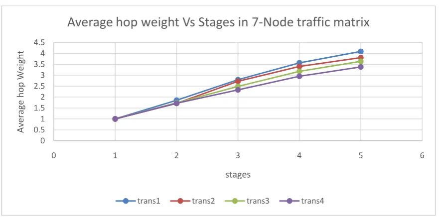
Fig3:7-Nodes, 4-Transceivers on stage wise Average hop Weight

In Fig-3, comparison takes place between Average hop Weight Vs. Stages with 4 transceivers. As the traffic is increased and usage of 2,3,4 transceivers, the average hop weight is gradually increased on 7-Node Traffic Matrix

Fig 4: 7-Nodes, 4- Transceivers comparison different stages Utilization of Wave lengths

In Fig-4 represents the utilisation of wavelengths on 7-node Traffic matrix with different stages with 4 transceivers. The Utilisation is effective when traffic matrix grows and as well as usage of 2-4transceivers

0 0.5 1 1.5 2 2.5 3 3.5 4 4.5

0 1 2 3 4 5 6

Av

erage

h

op

We

ig

h

t

stages

Average hop weight Vs Stages in 7-Node traffic matrix

trans1 trans2 trans3 trans4

0 10 20 30 40 50

0 1 2 3 4 5 6

Wav

e le

n

gth

stages

Utilisation of Wavelength - 7 Node traffic matrix

(8)

Heuri stic

no de

Tr An ScEi Vers

Lig ht Pat h

Wav elen th

Phy Hop Wei ght

Hop Wei ght

Total Hop weight

Average Hop weight

Maximum congestion

Min congestion

Stage1 14 1 13 0 13 860 860 1 2 -> 12 (98) 7 ->9(17) 14 2 27 1 27 1567 1567 1 2 -> 12 (98) 8 ->3(12) 14 3 40 3 40 2025 2025 1 8 -> 5 (114) 12 ->13(3) 14 4 53 5 53 2601 2601 1 0 -> 2 (192) 13 ->11(4) stage2 14 1 13 2 33 1572 4178 2.658 1 -> 10 (314) 4 ->1(70)

14 2 27 6 66 3033 8102 2.671 3 -> 1 (506) 11 ->2(58 14 3 40 12 94 4272 10754 2.517 10- 12 (645) 1 ->0(68) 14 4 53 18 120 5284 12742 2.411 1 -> 10 (773) 12 ->10(81) stage3 14 1 14 2 40 1627 4998 3.072 1 -> 4 (371) 1 ->0(56)

14 2 27 7 79 3258 9910 3.042 6 -> 9 (621) 2 ->11(95) 14 3 41 13 117 4813 14741 3.063 2 -> 5 (797) 12 ->10(81) 14 4 55 22 152 6184 18278 2.956 1 -> 10 (992) 12 ->10(81) stage4 14 1 14 2 42 1648 5359 3.252 2 -> 5 (427) _{1 ->0(56)}

14 2 28 8 87 3282 11063 3.371 2 -> 5 (862) 1 ->0(68) 14 3 42 16 122 4763 15097 3.17 2 -> 5 (1108) 2 ->0(136) 14 4 56 25 159 6251 19155 3.064 2 -> 5 (1244) 7 ->4(129) stage5 14 1 14 2 42 1648 5359 3.252 2 -> 5 (427) 1 ->0(56)

14 2 28 8 87 3282 11063 3.371 2 -> 5 (862) 1 ->0(68) 14 3 42 16 122 4763 15097 3.17 2 -> 5 (1108) 2 ->0(136) 14 4 56 25 159 6251 19155 3.064 2 -> 5 (1244) 7 ->4(129)

Table3: 14 Node (NSFNET) heuristic data table

0 93 96 ∞ ∞ ∞ ∞ ∞ ∞ ∞ ∞ ∞ ∞ ∞

39 0 ∞ 14 77 ∞ ∞∞ ∞ ∞ 44 ∞ ∞ ∞

78 ∞ 0 ∞ ∞ 39 ∞ ∞ ∞ ∞ ∞ 88 98 ∞

∞ 5 ∞ 0 ∞ ∞ 39 ∞ 25 ∞ ∞ ∞ ∞ ∞

∞ 26 ∞ ∞ 0 ∞ ∞ 28 ∞ 23 ∞ ∞ ∞ ∞

∞ ∞ 7 ∞ ∞ 0 ∞ 97 40 ∞∞ ∞ ∞ ∞

∞ ∞ ∞ 61 ∞ ∞ 0 ∞ ∞ 36 ∞ ∞ ∞ 42

∞ ∞ ∞ ∞ 61 49 ∞ 0∞ 17 ∞ ∞ ∞ ∞

∞ ∞ ∞ 12 ∞ 57 ∞ ∞ 0 ∞ ∞ ∞ ∞ ∞

∞ ∞ ∞ ∞ 42 ∞ 97 47 ∞ 0 ∞ ∞ ∞ ∞

∞ 29 ∞ ∞ ∞ ∞ ∞ ∞ ∞ ∞ 0 41 28 0

∞ ∞ 54 ∞ ∞ ∞ ∞ ∞ ∞ ∞ 67 0 ∞ 87

∞ ∞ 26 ∞ ∞ ∞ ∞ ∞ ∞ ∞ 81 ∞ 0 3

∞ ∞ ∞ ∞ ∞ ∞ 53 ∞ ∞ ∞ ∞ 4 58 0

(9)

Table-3 is on 14-node(NSFNET) traffic matrix with different stages is showing results on utilisation of transceivers, light paths wavelengths, hop weight, total hop weight, average hop weight, maximum congestion and min congestion.

Fig5:14-Nodes 4-Transceivers different stages on average hop weight

In Fig-5, comparison takes place between Average hop Weight vs. Stages with 4 transceivers. As the traffic is increased and usage of 2-4 transceivers the average hop weight is gradually increased on 14-Node (NSFNET) Traffic Matrix

Fig6:14-Nodes 4- Transceivers different stages on Utilization of Wave lengths

0 0.5 1 1.5 2 2.5 3 3.5 4

0 1 2 3 4 5 6

av

g h

o

p

w

eight

stages

Average hopweight Vs stages in14-Node Traffic Matrix

trans1 trans2 trans3 trans4

0 5 10 15 20 25 30

0 1 2 3 4 5 6

Wa

ve

le

n

gth

stages

Utilization of Wave length 14-node Traffic Matrix

(10)

In Fig-6 represents the utilisation of wavelengths on 14-node (NSFNET) Traffic matrix with different stages with 4 transceivers. The Utilisation is effective when traffic matrix grows and as well as usage of 2-4 transceivers

V.CONCLUSION

In this paper the main emphasis of this work to find all pair shortest path by using dynamic programing on virtual topology. All the nodes are chosen as sources in step by step to produce the fulfilled traffic to the given network, the existing physical topology to topology is not linked to the all nodes.

By taking the existing traffic matrix and applying dynamic programing as said above the stage wise traffic matrices are developed. And each stage the Heuristic Logical Design Algorithm was applied and observed the results. The method was implemented 4nodes, 7nodes and 14 NSFNET.

When compared average weighted hops in Fig-(1) for 2-transcievers the solution is optimum in all stages. In case of Fig-(3) & (5) the average weighted hops are gradually increasing as the number of Transceivers are increasing and as well as traffic is increasing.

Utilization of wave length in Fig-(2) gradually increasing in 4-node traffic .in Fig-(4) and (6) utilization of wave lengths is also increased as the traffic is going in stage wise. Hence it is concluded that when the demand of a traffic is enhanced the average weighted hops and utilization of wave lengths is also increased gradually.

REFERENCES

1. Chlamtac, I., Ganz, A. and Karmi, G ―Light path communication: A novel pproach to high bandwidth optical WAN’s‖ IEEE Transactions on Communications 40(7), 1171– 1182, [1992]. Chlamtac, I., Ganz, A. and Karmi, G ―Light nets: Topologies for high speed Optical networks,‖ IEEE/OSA Journal of Light wave Technology 11(5/6), 951–961, [1993].

2. Ramaswami, R. and Sivarajan, K. N. ―Routing and wavelength assignment in all Optical networks‖, IEEE/ACM Transactions on

Networking 3(5), 489–500,[1995]

3. Datta, R., Mitra, B., Ghose, S. and Sengupta, I. ―An algorithm for Optimal assignment of a wavelength in a tree topology and its

application in WDM Networks”, IEEE Journal on Selected Areas in Communications 22(9), 1589–1600. [2004]

4. Ram swami, R. and Siva rajan, K. N. ―Design of logical topologies for wavelength-Routed optical networks‖, IEEE Journal on Selected Areas in Communications, 14(5), 840–851,[1996]

5. Mukherjee, B., Banerjee, D., Ramamurthy, S. and Mukherjee, A. ―Some principles For designing a wide-area WDM optical network‖,

IEEE/ACM Transactions on Networking 4(5), 684–695, [1996]

6. Banerjee, D. and Mukherjee, B. ―Wavelength routed optical networks: Linear Formulation, Resource budget trades and a

reconﬁguration study‖, IEEE/AC Transactions on Networking 8(9), 598–607. [2000]

7. Ghose, S., Kumar. R., Banerjee and Dutta, R ―Multi hop ―Virtual topology design In WDM optical networks for self-similar traﬃc‖, Photonic Network Communications 10(2), 199–214, [2005].

8. Girvan & New- man,— a sub-problem of many combinatorial problems[2002]

9. HELD, M., and KARP, R. M.). "The construction of discrete dynamic programming Algorithms", IBM Systems Journal, Vol. 4, No. 2, p. 136 [1965]

BIOGRAPHY

(11)