ANDERSEN, BRIAN DOUGLAS. Development and Assessment of Multi-Objective Optimization Utilizing Genetic Algorithms for Nuclear Fuel Assembly Design. (Under the direction of Dr. David Kropaczek.)
MOOGLE, Multi-Objective Optimization utilizing Genetic algorithms for Lattice Enhancement, is a new genetic algorithm developed for the optimization of PWR and BWR fuel assemblies. MOOGLE advances the field of nuclear fuel management by using three-dimensional fuel rod types as the decision variables within the assembly optimization, instead of the standard two-dimensional pin cell lattice. Using fuel rod types as the genes within the genetic algorithm optimization framework allows whole assemblies to be optimized at once, rather than focusing on two-dimensional fuel lattices. Additionally, it allows core designers to easily see the economic tradeoffs between assembly performance and manufacturability through the addition of objective functions or constraints related to characteristics of the fuel rod types within the optimization, such as the number of unique rod types allowed in optimized designs.
A novel feature of the MOOGLE algorithm includes the use of a desired solution space and binning procedure to store valuable optimization solutions. MOOGLE additionally uses a tournament selection method for determining which solutions will be selected as the parents of the next generation. To preserve solution niching, solutions undergoing crossover seek to mate with solutions composed of similar rod types.
by comparing the results of optimizations using IFBA, gadolinium, and a combination of IFBA, as well as gadolinium for a PWR fuel assembly in octant symmetry with the same objectives as the sensitivity analysis. Finally, to demonstrate the MOOGLE’s ability to optimize entire fuel rod bundles, a whole BWR fuel bundle was optimized using MOOGLE.
Development and Assessment of Multi-Objective Optimization Utilizing Genetic Algorithms for Nuclear Fuel Assembly Design.
by
Brian Douglas Andersen
A thesis submitted to the Graduate Faculty of North Carolina State University
in partial fulfillment of the requirements for the degree of
Master of Science
Nuclear Engineering
Raleigh, North Carolina 2018
APPROVED BY:
_______________________________ _______________________________ Dr. David Kropaczek Dr. Jason Hou
Committee Chair
DEDICATION
iii BIOGRAPHY
Brian Andersen was born and raised in Billings, Montana. After graduating from Skyview High School in 2012, he attended Idaho State University. While at Idaho State University, Brian Andersen participated in the Washington Internship for Students of
Engineering. Through this program, he authored a policy paper on restarting the United States nuclear waste disposal program. Additionally, Brian Andersen became a licensed reactor operator for the AGN-201 nuclear reactor at Idaho State University. Mr. Andersen was also a member of the American Nuclear Society and Institute for Nuclear Materials Management. He served as secretary in the latter. He graduated from Idaho State University in 2016 with honors distinction, earning degrees in nuclear and mechanical engineering.
Brian Andersen is currently a graduate student at North Carolina State University, working under the supervision of Dr. David Kropaczek. His research focuses on artificial optimization and machine learning to improve nuclear fuel assembly designs.
ACKNOWLEDGMENTS
I would like to thank North Carolina State University and the nuclear engineering department for providing the resources for this research. A special thank you to Dr. Kropaczek for all of his help, wisdom, and guidance in the development of MOOGLE. Hermine also deserves a warm thank you as well for all of her organizing my life in these past few months to allow this research to be completed. Thank you to Dr. Hou, Mario, and Dr. Baelustra for putting up with all of the weird things I try to do to the cluster. Finally, I would like to thank the
v TABLE OF CONTENTS
LIST OF TABLES ... vi
LIST OF FIGURES ... vii
LIST OF ACRONYMS AND ABBREVIATIONS ... x
Chapter 1 INTRODUCTION ... 1
1.1 Overview ... 1
1.2 Literature Review ... 4
1.3 Casmo4e ... 6
Chapter 2 MOOGLE ALGORITHM DESCRIPTION ... 7
2.1 Brief Description of Genetic Algorithms ... 7
2.2 Genes, Genomes, and Chromosomes ... 8
2.3 Population Size ... 10
2.4 Initialization Population Creation ... 11
2.5 Survival ... 12
2.6 Parent Selection ... 16
2.7 Reproduction ... 18
2.8 End of Optimization Conditions ... 21
2.9 MOOGLE Flowchart... 21
Chapter 3 MOOGLE ALGORITHM TESTING ... 23
3.1 PWR Optimization Description ... 23
3.2 BWR Optimization Description ... 30
Chapter 4 EXPERIMENTAL RESULTS ... 35
4.1 PWR Geometry Solution Front Test Case ... 35
4.2 Burnable Poison Analysis Results ... 36
4.3 BOC BWR Problem ... 44
4.4 Depletion and Multiple Zone BWR Problem ... 47
Chapter 5 Analysis of Results ... 52
5.1 Burnable Poison Analysis Discussion ... 52
5.2 BOC BWR Optimization Discussion ... 56
5.3 Depletion and Multiple Zone BWR Problem ... 58
Chapter 6 Conclusions ... 60
Chapter 7 References ... 63
LIST OF TABLES
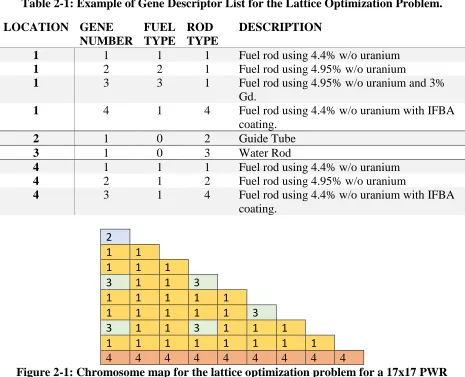
Table 2-1: Example of Gene Descriptor List for the Lattice Optimization Problem... 9
Table 3-1: Rod List for the PWR Lattice Optimization Problem. ... 24
Table 3-2: Operating conditions used in Casmo4e for PWR lattice physics calculations. ... 24
Table 3-3: Selection Weights Used in Sensitivity Analysis. ... 26
Table 3-4: Initial and Final Mutation Rates Used in Sensitivity Analysis Optimizations ... 26
Table 3-5: Bin Sizes Used in Sensitivity Analysis Optimizations ... 26
Table 3-6: Population Sizes and Maximum Generations Used in Sensitivity Analysis Optimizations ... 26
Table 3-7: Population Sizes and Maximum Generations Used in BP Analysis Optimizations.... 26
Table 3-8: Allowed Solution Space for SA and BP Optimizations ... 27
Table 3-9: Rod List for the first BWR Optimization Problem. ... 32
Table 3-10: Rod List for the second BWR Optimization Problem. ... 34
Table 4-1: Number of Generations for Burnable Poison Analysis ... 37
Table 4-2: Minimum, Maximum, and Average Parameter Values for BOC BWR Optimization ... 46
Table 4-3: Number of Generations for the Second BWR Optimization Problem ... 47
Table 4-4: Average Objective Values for the Second BWR Optimization Problem ... 47
Table 4-5: Minimum Objective Values for the Second BWR Optimization Problem ... 48
Table 4-6: Maximum Objective Values for the Second BWR Optimization Problem... 48
Table 4-7: Percentage of Rod Types Used in Second BWR Optimization ... 51
Table 5-1: Average Distance Comparison of IFBA and Gad Only ... 52
Table 5-2: Comparison of MOOGLE algorithm results to the Mustang Algorithm ... 57
Table 5-3: Distance between the three cases of the second BWR optimization problem ... 58
Table A-0-1: Number of Generations for Sensitivity Analysis Cases ... 66
Table A-0-2: Averaged Average Final Population Metrics for Sensitivity Analysis ... 67
Table A-0-3: Average Minimum Final Population Metrics for Sensitivity Analysis ... 68
vii LIST OF FIGURES
Figure 1-1: Fuel loading pattern for a nuclear reactor core [5]. ... 3
Figure 1-2: Axial distribution of fuel bundle where each axial level represents one neuron. ... 6
Figure 2-1: Chromosome map for the lattice optimization problem for a 17x17 PWR assembly. ... 9
Figure 2-2: First four solutions within initialization population for example problem. ... 12
Figure 2-3: Example of a two objective Pareto front [19]. ... 13
Figure 2-4: Flow chart for binning survival process ... 15
Figure 2-5: Flow chart of parent selection process. ... 17
Figure 2-6: Reproduction selection method flow chart. ... 18
Figure 2-7: Crossover Illustration. ... 20
Figure 2-8: Overall flow chart for the MOOGLE algorithm. ... 22
Figure 3-1: Rod zone region map for the PWR geometry problem. ... 23
Figure 3-2: Depiction of epsilon indicator distance test. ... 28
Figure 3-3: Example of a combined solution front obtained from two different solution fronts. ... 29
Figure 3-4: A: Axial power and void as functions of height. B: Positions of BWR axial regions for first and second BWR optimization problems. ... 31
Figure 3-5: Rod zone region map for the first BWR optimization problem. ... 32
Figure 3-6: Rod zone region map for the second BWR optimization problem. ... 33
Figure 3-7: The R-factor is function of the surrounding rod power. ... 35
Figure 4-1: Comparison of a binned solution front to the Optimal Pareto Front for the optimization of a small number of rods at beginning of cycle. ... 36
Figure 4-2: Base Case Solution Space Results. ... 38
Figure 4-3: IFBA Only Solution Space Results. ... 39
Figure 4-4: Gadolinium Only Solution Space Results. ... 40
Figure 4-5: BP use in Optimizations using three different rod sets. ... 41
Figure 4-6: Average percentage of lattice solutions in final population using each rod type for the three rod set optimizations. ... 42
Figure 4-7: Lattice Solution combining IFBA and gadolinium as burnable poisons.. ... 43
Figure 4-8: Lattice Solution using only IFBA as burnable poison. ... 43
Figure 4-9: Lattice Solution using only gadolinium as burnable poison. ... 44
Figure 4-10: Solution space of the BOC BWR lattice optimization problem. ... 45
Figure 4-11: Lattice Solution with lowest R factor produced by MOOGLE Algorithm using 9 rod types for the BOC BWR optimization problem. ... 46
Figure 4-12: Lattice Solution with lowest R factor produced by MOOGLE Algorithm using 9 rod types at a BOC Kinf value near 1.20 for the BOC BWR optimization problem. ... 46
Figure 4-13: Number of Counts per bin for the second BWR problem eighteen rod case. ... 48
Figure 4-14: Number of counts per bin for the second BWR problem for the fifteen-rod case. .. 49
Figure 4-15: Number of counts per bin for the second BWR problem for the twelve-rod case. .. 49
Figure 4-16: Comparison of rod types used by the three different optimization cases for the second BWR optimization problem. ... 50
Figure 5-1: Solution Front and Solution space comparison between base and the IFBA
only test cases. ... 53
Figure 5-2: Solution Front and Solution space comparison between base and the gadolinium only test cases.. ... 54
Figure 5-3: Solution Front and Solution space comparison between base, ifba only, and gadolinium only test cases. ... 55
Figure 5-4: Solution front curve for BOC BWR optimization problem. ... 57
Figure 5-5: Solution front for the 12, 15, and 18 rod cases of the second BWR optimization problem. ... 58
Figure 5-6: Comparison of the Solution spaces covered by the three different rod cases. ... 59
Figure A-1: Selection Weight One Solution Space Results... 69
Figure A-2: Selection Weight Two Solution Space Results.. ... 70
Figure A-3: Selection Weight Three Solution Space Results. ... 71
Figure A-4: Selection Weight Four Solution Space Results. ... 72
Figure A-5: Selection Weight Five Solution Space Results. ... 73
Figure A-6: Selection Weight Six Solution Space Results. ... 74
Figure A-7: Small Population One Solution Space Results... 75
Figure A-8: Small Population Two Solution Space Results. ... 76
Figure A-9: First Alternate Mutation Rate One Solution Space Results.. ... 77
Figure A-10: Second Alternate Mutation Rate Two Solution Space Results.. ... 78
Figure A-11: Large PPF Bin Size Solution Space Results. ... 79
Figure A-12: Large Peak Kinf Bin Size Solution Space Results.. ... 80
Figure A-13: Large EOC Kinf Bin Size Solution Space Results. ... 81
Figure A-14: Solution Front and Solution space comparison between base and first select weight test cases. ... 83
Figure A-15: Solution Front and Solution space comparison between base and second select weight test cases... 84
Figure A-16: Solution Front and Solution space comparison between base and third select weight test cases... 85
Figure A-17: Solution Front and Solution space comparison between base and fourth select weight test cases.. ... 86
Figure A-18: Solution Front and Solution space comparison between base and fifth select weight test cases. ... 87
Figure A-19: Solution Front and Solution space comparison between base and sixth select weight test cases. ... 88
Figure A-20: Solution Front and Solution space comparison between base and first small population test cases. ... 90
Figure A-21: Solution Front and Solution space comparison between base and second small population test case. ... 91
Figure A-22: Solution Front and Solution space comparison between base and first alternate mutation rate cases. ... 93
Figure A-23: Solution Front and Solution space comparison between base and second alternate mutation rate cases. ... 94
ix Figure A-25: Solution Front and Solution space comparison between base and the large
peak kinf bin size. ... 97 Figure A-26: Solution Front and Solution space comparison between base and the large
LIST OF ACRONYMS AND ABBREVIATIONS MWD/MTU Mega-Watt day per metric ton uranium
U.S. NRC United States Nuclear Regulatory Commission PWR Pressurized water reactor
BWR Boiling water reactor
IFBA Integral fuel burnable absorber
GA Genetic algorithm
MOO Multi objective optimization
FORMOSA-P Fuel Optimization for Reloads – Multiple Objectives by Simulated Annealing - PWR
NCSU North Carolina State University PPF Power Peaking Factor
BOL Beginning of Life
EOC End of Cycle
CPR Critical Power Ratio SA Sensitivity Analysis
1 Chapter 1INTRODUCTION
1.1 Overview
Nuclear fuel management is the production, use, and disposal of fuel used by nuclear reactors. A principle focus of the field is the economical design of nuclear fuel assemblies that meet the operational and safety constraints of nuclear reactors. These designs must incorporate factors such as higher burnups, effective reactivity management, and the utilization of standardized fuel rod types in order to create a wide array of fuel bundles. Incorporation of these factors improves the cost of fuel bundles and nuclear reactors [1]. Safety constraints include limits on FΔH and Fq, the radial and axial power peaking, as well as limits on core reactivity. Other safety constraints include maintaining safety margins for issues such as minimum departure from nucleate boiling and dryout [1]. Often, satisfying these safety constraints forces sacrifices in cost factors. Therefore, core designers must strike the right balance; designing fuel that minimizes manufacturing costs, maximizes profits, and meets all safety constraints.
multiplication factor at unity [3]. This means that methods must be implemented to control this reactivity.
The first method for controlling reactivity is the use of poisons. Reactivity poisons in a pressurized water reactor (PWR) core include control rods in the reactor core, chemical shim added to the reactor moderator, and burnable poisons within fuel rods in the assemblies. Boiling water reactors (BWR) rely solely on control rods and burnable poisons in the fuel bundle. Both BWRs and PWRs use gadolinium as a burnable poison. Gadolinium is placed in select fuel rods and uses set combinations of Gd2O3-UO2 to form the control material [1]. IFBA, a coating of zirconium diboride (ZrB2) applied to the outside of fuel pellets, is another burnable poison specific to PWRs that was developed by Westinghouse for the VANTAGE-5 fuel [4]. Burnable poison placement is vital for fuel assembly design, as the same poison in different locations within a fuel assembly will have drastically different effects on pin powers and reactivity within the fuel assembly. Additionally, the cost of burnable poisons makes it desirable to use as little as possible to achieve the desired decrease in reactivity [1].
The second method for controlling reactivity is the use of complicated core loading patterns, such as the one shown in Figure 1-1, to utilize already “burnt” fuel with lower excess fuel reactivity in combination with new fuel to reduce the overall core average excess reactivity. Greater flexibility in the number of assemblies used in the core allows for greater management of the radial reactivity peaking and improves the burnup of all fuel used in the reactor core. Greater numbers of fuel assemblies can come at a steep price however as the numbers of specific rod types and enrichments increases.
3 assemblies increases the difficulty further. This difficulty motivates the proposal of a new genetic algorithm, MOOGLE, for the design of nuclear fuel assemblies.
Figure 1-1: Fuel loading pattern for a nuclear reactor core [5].
1.2 Literature Review
The survey of previous work shows genetic algorithms are not new to nuclear fuel management. Fuel lattices for PWRs and BWRs have been optimized using a variety of methods, including genetic algorithms. Three-dimensional assemblies have also been optimized.
Martin-del-Campo et. al. developed a genetic algorithm capable of optimizing the enrichments and gadolinium concentrations in a BWR radial lattice. Their optimization sought to: (1) minimize the average lattice enrichment, (2) achieve an average gadolinium concentration G(x) equal to a target Gtarget, (3) achieve an infinite multiplication factor kinf equal to the target Kinf target, and (4) to attain a power peaking factor (PPF) lower than a limit value PPFmax, and if possible, to minimize it [6]. Information on kinf and PPF were obtained using the neutronic simulator Helios developed by Studsvik Scandpower [7].
A multi-objective fitness function determined the value of different solutions in their optimization. Their fitness function is presented in Equation 1.1 [6]. The fitness function used by Martin-del-Campo et al is complex, involving finally tuned weights and sub equations to measure the fitness of each solution in the optimization. The use of fitness functions such as these is undesirable, because they essentially limit the algorithm to only being able to solve one problem. Should a new optimization objective be introduced, the entire fitness function must be re-tuned.
𝐹(𝑥) = 𝐶 + 𝑤𝐸∗ 𝐸(𝑥) + 𝑤𝐺∗ ∆𝐺(𝑥) + 𝑤𝑝∗ (𝑃𝑃𝐹(𝑥) − 𝑃𝑃𝐹𝑚𝑎𝑥) + 𝑤𝑘∗ 𝐷𝑘(𝑥) 1.1
5 methods. Their results depicted that Greedy Searches produced the best lattice designs, but GAs and Path Relinking were the two best methods in terms of global cost and reliability [8]. This shows that GAs remain a powerful optimization method.
Rogers et al used adaptive simulated annealing (ASA) to optimize the radial pin enrichments and burnable poisons in a PWR fuel lattice [9]. ASA is an open source code written in C [10]. Simulated annealing is another artificial optimization method like GA’s. Simulated annealing is based on the natural process of materials cooling from high to low temperature, ultimately reaching the lowest achievable energy state [9].
Rogers et al minimized the PPF of a 15 x 15 lattice in octant symmetry at beginning of life. Their optimization included standard design constraints such as prohibiting placement of gadolinium bearing pins in periphery locations and holding water rod and instrument tube locations fixed. Two heuristic rules were implemented that limited the locations of where gadolinium bearing pins could be placed based on a correlation between gadolinium placement and PPF [9].
Similar to Martin-del-Campo et al, Rogers et al used a complex fitness function in their optimization. Additionally, ASA evaluated a large number of solutions to optimize the different cases evaluated, and only produced one optimal solution for each case analyzed [9].
Simulate-3 were used to analyze the two dimensional lattices and three dimensional fuel bundles respectively [12] [13].
GreeNN successfully optimizes the reactor physics and safety limits of three-dimensional fuel bundles; however, GreeNN is not applicable to real world design problems. Figure 1-2 shows the axial layout used in the optimization, where each neuron is one axial fuel level [11]. Each color in Figure 1-2 describes a different zone in which fuel lattices may be placed. Based on the GreeNN system, each of these axial zones would be composed of a different two dimensional lattice. This means each fuel rod used in the fuel bundle is unique. This means high manufacturing costs for building fuel bundles designed by GreeNN. Manufacturing multiple fuel bundles based off of GreeNN for use in one reload batch would be economically impossible.
Figure 1-2: Axial distribution of fuel bundle where each axial level represents one neuron. 1.3 Casmo4e
All lattice physics calculations were performed using Casmo4e. Casmo-4 is a multigroup two-dimensional transport theory code for burnup calculations on BWR and PWR assemblies. The code geometry utilizes cylindrical fuel rods in a square pitch array and can handle a variety of fuel materials [12].
The two-dimensional transport solution uses the method of characteristics and can be carried out using several different energy group structures. A seventy-energy group library covering the energy range 0 to 10 MeV stores the nuclear data. Casmo4e handles thermal expansion automatically and calculates resonance cross sections for each individual pin. A fundamental mode calculation incorporates leakage affects [12].
7 approach calculates depletion, which greatly reduces the number of steps without reducing accuracy [12].
Chapter 2 MOOGLE ALGORITHM DESCRIPTION
The MOOGLE algorithm advances the field of nuclear fuel management by using rod types as the genes and rod maps to define the problem. For purposes of MOOGLE, the number of unique fuel rod types is a proxy for manufacturing cost. Binning of the solution space is also novel. MOOGLE provides a simple optimization framework readily available to solve a wide range of lattice optimization problems. By using rod types as the decision variable, and using a simple fitness method based on ranking, the MOOGLE algorithm can solve two-dimensional lattice optimization problems just as easily three-dimensional fuel assembly optimization problems without any changes to the algorithm. Binning of the solution space allows designers to see all of the different designs, as well as their strengths and weaknesses side by side in order to select the designs that work best for them within the core loading pattern. Additionally, use of rod types as the decision variable allows designers to see the tradeoffs between cost and performance for various numbers of rod types. These advancements make the MOOGLE optimization algorithm a novel contribution to the field of nuclear fuel management.
2.1 Brief Description of Genetic Algorithms
GAs apply to a range of problems such as game playing, function optimization, and search optimization of large scale combinatorial optimization problems like nuclear fuel lattice design or the well-known traveling salesman problem. GAs are adept for parallel programming, allowing a large section of the solution space to be searched quickly and provide a wide array of different solutions [14]. A disadvantage of GAs are that they provide no proof an optimum solution has been found [8]. Goldberg notes that GAs do not necessarily reach the best solution within the space and that combining GAs with another search method such as Tabu searches often yields better results than the GA search alone [14]. GAs also propagate undesirable solutions for several generations, which wastes computational resources [6].
2.2 Genes, Genomes, and Chromosomes
Genetic algorithms utilize a genome. The genome, typically a string of characters or binary numbers, represents all the information of a solution, and can be modified to create new solutions through the manipulation of genes, which represent individualized aspects of the problem [14].
The fuel assembly design problem is a placement problem where the optimal fuel rod type configuration for the fuel assembly is sought. The MOOGLE algorithm utilizes a gene pool and chromosome map to describe solution genomes. The gene pool describes the physical characteristics of the fuel rods used in the optimization. The gene pool also states which genes are allowed on which chromosomes. The chromosome map divides the geometry of the fuel assembly design problem into different radial regions that define where rod types may or may not be used in the solution of the design problem.
9 designating the guide tubes and water rods as individual chromosomes with one allowed gene on that chromosome, these items are held fixed within the problem. Second, all fuel genes may be expressed in the chromosome 1. Third, the fuel gene containing gadolinium may not be expressed in chromosome 4. These observations demonstrate the simplicity of describing a problem within the MOOGLE framework.
Table 2-1: Example of Gene Descriptor List for the Lattice Optimization Problem. LOCATION GENE
NUMBER FUEL TYPE ROD TYPE DESCRIPTION
1 1 1 1 Fuel rod using 4.4% w/o uranium
1 2 2 1 Fuel rod using 4.95% w/o uranium
1 3 3 1 Fuel rod using 4.95% w/o uranium and 3% Gd.
1 4 1 4 Fuel rod using 4.4% w/o uranium with IFBA coating.
2 1 0 2 Guide Tube
3 1 0 3 Water Rod
4 1 1 1 Fuel rod using 4.4% w/o uranium
4 2 1 2 Fuel rod using 4.95% w/o uranium
4 3 1 4 Fuel rod using 4.4% w/o uranium with IFBA coating.
2
1 1
1 1 1
3 1 1 3
1 1 1 1 1
1 1 1 1 1 3
3 1 1 3 1 1 1
1 1 1 1 1 1 1 1
4 4 4 4 4 4 4 4 4
Figure 2-1: Chromosome map for the lattice optimization problem for a 17x17 PWR assembly.
PWR fuel assemblies contain top and bottom blanket regions, as well as burnable absorber cutback regions; however, optimizing only the radial fuel lattice extending over the dominant central axial region is sufficient to optimize the entire assembly. Optimization of BWR fuel bundles, on the other hand, involves multiple radial fuel lattices extending over several axial fuel regions. MOOGLE can easily optimize both problems through the implementation of the gene pool which utilizes rod types and chromosome map.
2.3 Population Size
Population sizes depend on a variety of factors including computational resources and problem complexity. The population of multiple solutions allows GA’s to search a large breadth of the solution space, and the population of solutions also helps the optimization to escape from local optimal solutions. If a GA uses too small of a population, convergence will occur too quickly; too large of population’s waste computational resources [15].
MOOGLE calculates population size based off of the formula used in FORMOSA-P [16]. Population size is determined by the total number of possible genes. The total number of possible genes are the sum of all genes that may be expressed in a given gene location over the entire genome. For the lattice optimization problem, this is the sum of all the different rod types allowed in a given location for all rod positions. Population size is calculated as:
𝑁𝑝𝑜𝑝≈ 10 ∗ √𝑁𝑔𝑒𝑛𝑒𝑠 2.1
11 𝑁𝑔𝑒𝑛𝑒𝑠 = 30 ∗ 4 + 1 ∗ 1 + 5 ∗ 1 + 9 ∗ 3 = 153
The square root of one hundred fifty-three, rounded to the nearest whole number is: √153 ≈ 12
The population size for our example is then one hundred twenty. 2.4 Initialization Population Creation
Traditionally, random solutions from the available gene pool compose the initial population [14]. The MOOGLE algorithm does not follow this approach. Instead, the MOOGLE algorithm uses every homogeneous combination of chromosomes to form the initialization population.
Figure 2-2 illustrates this for the example problem. As the figure shows, the first four solutions in the initial population would be comprised of the three possible genes allowed in chromosome 4, indicated in red, combined with the first gene allowed in chromosome 1, indicated in gold. The sequence then repeats, now with the second allowed gene in chromosome 1. Chromosomes 2 and 3 remain constant because only one gene is allowed in these locations. The total initialization population size for the example problem would be twelve solutions.
A homogenous or semi-homogeneous genome is likely to be close to the optimized solution for one of the optimization parameters, motivating this decision. Using a good, non-random initialization population to produce the starting population significantly reduces the computational time over a random, relatively bad, initial population, especially for the lattice optimization problem.
From an optimization standpoint, it makes no sense to waste computational resources by starting with an infeasible population of solutions. The use of an initialization population created through homogeneous combinations of chromosomes allows the optimization to have a better starting population without the need for overcomplicated heuristic settings or in-depth knowledge of the problem.
1 1
1 1 1 1
1 1 1 1 1 1
1 1 1 1 1 1 1 1
1 1 1 1 1 1 1 1 1 1
1 1 1 1 1 1 1 1 1 1 1 1
1 1 1 1 1 1 1 1 1 1 1 1 1 1
1 1 1 1 1 1 1 1 1 1 1 1 1 1 1 1
1 1 1 1 1 1 1 1 1 2 2 2 2 2 2 2 2 2
First solution generated Second solution generated
1 1
1 1 2 2
1 1 1 2 2 2
1 1 1 1 1 2 2 1
1 1 1 1 1 2 2 2 2 2
1 1 1 1 1 1 2 2 2 2 2 1
1 1 1 1 1 1 1 1 2 2 1 2 2 2
1 1 1 1 1 1 1 1 2 2 2 2 2 2 2 2
3 3 3 3 3 3 3 3 3 1 1 1 1 1 1 1 1 1
Third solution generated Fourth solution generated
Figure 2-2: First four solutions within initialization population for example problem. 2.5 Survival
13 optimal solution tradeoffs for competing objectives, with solutions on the Pareto front being non-dominated by any other solutions to the optimization problem [18]. An example of a Pareto front is provided in Figure 2-3.
Figure 2-3:Example of a two objective Pareto front [19].
didn’t require complex tuning of a fitness function and preserved solutions that, although dominated by other solutions, still held value to a core designer.
Figure 2-4 shows the steps of the binning survival process. Calculate a fitness for each solution based on Equation 2.2. The number of bins is calculated using Equation 2.3. The bin in which each solution is placed is calculated using Equation 2.4.
𝐹 = ∑ 𝑤𝑖𝑅𝑖 𝑁𝑜𝑏𝑗𝑒𝑐𝑡𝑖𝑣𝑒𝑠
𝑖=1 2.2
Where wi is a user supplied importance ranking to that objective, and Ri is the rank of that solution for that optimization objective.
𝑁𝑏𝑖𝑛𝑠 =objmaximum−𝑜𝑏𝑗𝑚𝑖𝑛𝑖𝑚𝑢𝑚
𝑤𝑖𝑑𝑡ℎ𝑜𝑏𝑗 2.3
Where objmaximum is the maximum value of the objective currently existing within the allowed solution space, objminimum is the minimum value for that objective that currently exists within the solution space, and widthobj is the desired width of each bin for that objective.
𝐵𝑖𝑛# =
objscore−𝑜𝑏𝑗𝑚𝑖𝑛𝑖𝑚𝑢𝑚 𝑤𝑖𝑑𝑡ℎ𝑜𝑏𝑗
2.4
15
Reducing computational time by only using the minimum number of bins required motivates the use of Equation 2.3. Two possible methods were identified for the binning process. The first method used a fixed number of bins, while the second method used a fixed bin size. Fixed bin sizes are used over a fixed number of bins because fixed bin sizes provide better resolution
over the solution space by being able to add or remove needed bins. This enhanced resolution makes it easier to identify valuable solutions and provides clarity of the current solution space to the designer.
The overall motivation for binning is to reduce the number of solutions that are kept in the optimization. All solutions within the same final bin should be thought of as having equal value. Using a fitness is simply a convenient means for choosing a solution to represent the binned space. 2.6 Parent Selection
Determining which solutions pass their genes on to the next generation is one of the core parts of a genetic algorithm [14]. The MOOGLE algorithm uses a somewhat complicated method to decide which solutions in the desired solution space should act as the parents to the next generation of solutions. A flow chart for the parent selection process can be found in Figure 2-5.
17
2.7 Reproduction
The final key element of GA’s so far undiscussed is generating new child solutions from the selected parent population. GA’s utilize crossover and mutation to create the next generation of children [14]. The three specific reproduction methods used in the MOOGLE optimization algorithm are crossover, single mutation, and double mutation. The process used for determining how parents reproduce in the MOOGLE algorithm is illustrated in Figure 2-6.
Figure 2-6: Reproduction selection method flow chart.
19 program by mating similar genomes that to one another. In breeding programs, it is beneficial to select animals with similar traits as mates for each other. Selecting mates with similar characteristics allows traits within the mates to be expressed faster than through random mating. This allows undesirable traits to be identified and removed faster [22].
This method has a second advantage. Crossing over two solutions that both have high fitness values but differing genomic structure rarely result in children of note [14]. Another way of saying this is that if two solutions are on differing peaks within the solution space, any children these solutions have are more likely to result in the valley between the solutions, rather on an undiscovered, higher peak than the parents.
Crossover in the MOOGLE algorithm replicates a breeding program by mating the most similar genomes together. All parents designated for crossover are stored in a list. The first parent in the list is taken as the first parent to be used in the crossover pair. The rest of the parents in the crossover list are then examined to find the most suitable mate. For each parent, the genome is analyzed to determine how many genes it has in common with the first parent. This means having the same gene in the location within the genome. The genome that has the most genes in common with the first parent is chosen as the most suitable mate and second parent used in crossover.
rod type differs from that of the crossover lattice. Because there are fewer differences between the 1st potential mate and the crossover lattice versus the 2nd potential mate, the 1st potential mate is selected as the most suitable partner for crossover. The second row of lattices represent the children created in crossover. The green squares represent locations in which genes (rod types) were swapped between genomes. The 1st child lattice originally was the crossover lattice. The 2nd child lattice originally was the 1st potential mate. Once a parent has successfully crossed over with another parent in the crossover list, both parents are deleted from the crossover list.
0 0 0
1 0 1 0 1 0
1 0 0 1 0 0 1 0 0
1 1 3 1 1 2 3 1 1 4 3 1
1 1 1 1 7 1 2 3 3 7 1 4 1 3 7
1 1 1 8 8 7 1 1 1 8 8 7 1 4 1 8 8 7
1 1 3 8 8 1 1 1 1 3 8 8 1 1 1 3 3 8 8 1 1
1 1 1 3 1 3 1 1 1 1 1 3 1 3 1 1 1 3 3 3 1 3 1 1
1 5 1 7 1 1 7 1 7 1 5 1 7 1 1 7 1 7 1 5 1 7 1 1 7 1 7
0 1 1 1 1 1 1 1 1 0 0 1 1 1 1 1 1 1 1 0 0 1 1 1 1 1 1 1 1 0
First Parent First Possible Mate Second Possible Mate
0 0
1 0 1 0
1 0 0 1 0 0
1 2 3 1 1 1 3 1
1 1 1 3 7 1 2 3 1 7
1 1 1 8 8 7 1 1 1 8 8 7
1 1 3 8 8 1 1 1 1 3 8 8 1 1
1 1 1 3 1 3 1 1 1 1 1 3 1 3 1 1
1 5 1 7 1 1 7 1 7 1 5 1 7 1 1 7 1 7
0 1 1 1 1 1 1 1 1 0 0 1 1 1 1 1 1 1 1 0
First Child Solution Second Child Solution
Figure 2-7: Crossover Illustration.
21 of available rod types. For single mutation, this process occurs once, and for double mutation this process occurs twice.
Initial and final mutation rates are selected by the user. The mutation rate increases every generation based on the FORMOSA-P method [16]. Equations 2.5 and 2.6 are implemented within MOOGLE for determining the increase in the mutation rate each generation. The increase is based on the maximum number of possible generations for the optimization. This means that the target final mutation rate is often not achieved, as the solution space normally converges before the maximum number of generations is reached.
pmuten+1 = 1 − λg(1 − pmuten ) 2.5
Where pmuten and p mute
n+1 are the mutation rates for the n and n+1 generations and λ
g is a multiplier
calculated as:
λs = exp (𝑙𝑛((1−𝑝𝑓𝑖𝑛𝑎𝑙)(1−𝑝0))
𝑁𝑔𝑒𝑛 ) 2.6
2.8 End of Optimization Conditions
There are two conditions that can be met for the MOOGLE algorithm to stop. The MOOGLE algorithm is considered converged when less than ten new solutions have been added to the solution space in the last five generations. If MOOGLE is considered converged, the optimization ends. The other condition is for the maximum number of generations to be reached. MOOGLE will end after that final generation. The maximum number of generations is calculated similarly to population size, using the equation:
𝑁𝑚𝑎𝑥 _𝑔𝑒𝑛 ≈ 5 ∗ √𝑁𝑔𝑒𝑛𝑒𝑠 2.7
2.9 MOOGLE Flowchart
23
Chapter 3MOOGLE ALGORITHM TESTING
The MOOGLE algorithm was tested using two different assembly geometries, PWR and BWR. The PWR geometry was used to demonstrate the effectiveness of the binning method over Pareto sorting, to test the sensitivity of the algorithm to different parameters, and to analyze how the use of different BP combinations alter the results of the optimization. BWR geometry was used to compare the MOOGLE algorithm to a previously developed optimization algorithm, and to demonstrate the full fuel rod optimization capability and demonstrate the tradeoff between manufacturing complexity and increased performance through the addition of rod types.
3.1 PWR Optimization Description
The PWR geometry utilized a 17x17 fuel lattice in octant symmetry. The zone region map for the PWR optimization problem is provided in Figure 3-1. Two manufacturing design constraints were used to develop the rod zone regions: (1) The locations of guide tubes and water rods were held in fixed positions. (2) Gadolinium rods were restricted from edge pin cell
locations. The rod types used in the optimization are provided in Table 3-1. Lattice designs were depleted for a burnup of 20 MWD/MTU. Reactor conditions at which the lattice designs were run is provided in Table 3-2.
2
1 1
1 1 1
3 1 1 3
1 1 1 1 1
1 1 1 1 1 3
3 1 1 3 1 1 1
1 1 1 1 1 1 1 1
4 4 4 4 4 4 4 4 4
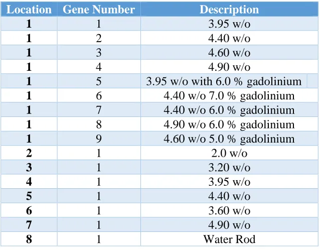
Table 3-1: Rod List for the PWR Lattice Optimization Problem.
Location Gene Description
1, 4 1 Fuel rod with 4.40 % w/o uranium
1, 4 2 Fuel rod using 4.95% w/o uranium
1 3 Fuel rod using 4.40% w/o uranium and 1% gadolinium 1 4 Fuel rod using 4.95% w/o uranium and 1% gadolinium 1 5 Fuel rod using 4.40% w/o uranium and 2% gadolinium 1 6 Fuel rod using 4.95% w/o uranium and 2% gadolinium 1 7 Fuel rod using 4.4% w/o uranium and 3% gadolinium 1 8 Fuel rod using 4.95% w/o uranium and 3% gadolinium 1, 4 9 Fuel rod using 4.40% w/o uranium with IFBA coating. 1, 4 10 Fuel rod using 4.95% w/o uranium with IFBA coating.
2 1 Guide Tube
3 1 Water Rod
Table 3-2: Operating conditions used in Casmo4e for PWR lattice physics calculations.
Power 110
Moderator 600
Fuel 820.5
Boron 900
Three experiments were conducted through the optimization of the PWR fuel assembly. The first experiment demonstrated how binning the solution space alters the results of an optimization over using a simple Pareto surface. The second experiment determined the sensitivity of the MOOGLE algorithm to different settings such as bin size or mutation rate. The third experiment determined how the inclusion of different burnable poison types affects the results of the optimization. To compare a solution binning method to a Pareto front method for carrying solutions forward in the optimization, a PWR fuel assembly was optimized at BOC, with the objectives of minimizing peak pin power and minimizing Kinf using a Pareto sorting method based on the method proposed by K.K. Mishra and Sandeep Harit [23].
25 optimization results. Two cases tested the effects of alternate mutation rates on the optimization results. The final three cases tested how bin size for various parameters affected the optimization results. All sensitivity test cases were compared to a standard base case. For each case, five runs were used to create the analysis dataset.
The selection weights used for each case are presented in Table 3-3. The mutation rates for all cases are presented in Table 3-4. The bin sizes for all cases are presented in Table 3-5. Each case used equal survival rates set at a value of one. All cases except the population size test case used Equation 2.7 to calculate the population size and maximum number of generations. The small population test size cases used Equation 3.1 to calculate population size. The first small population size test case also used equation to calculate the maximum number of generations.
𝑁𝑝𝑜𝑝 = 5 ∗ √𝑁𝑔𝑒𝑛𝑒𝑠 3.1
𝑁𝑔𝑒𝑛= 2.5 ∗ √𝑁𝑔𝑒𝑛𝑒𝑠 3.2
Population sizes and maximum number of generations for the cases are presented in Table 3-6. The allowed solution space for the selection weight analysis cases and BP analysis cases are presented in Table 3-8. Note that in Table 3-3 through Table3-8, if a case is not listed, its parameters are identical to the base case. Since the solution space size was altered for the bin size test cases, convergence would happen before the population was fully optimized. For this reason, these cases were set to run for the average number of generations used by the base optimization case.
case was the base case used in the sensitivity analysis. Population sizes and the maximum number of generations for the BP test cases are presented in Table 3-7.
Table 3-3: Selection Weights Used in Sensitivity Analysis.
Test Case Number Peak Pin Power Weight Peak Kinf Weight EOC Kinf Weight
Base 1 1 1
Selection Weight One 1 0 0
Selection Weight Two 0 1 0
Selection Weight Three 0 0 1
Selection Weight Four 1 1 0
Selection Weight Five 1 0 1
Selection Weight Six 0 1 1
Table 3-4: Initial and Final Mutation Rates Used in Sensitivity Analysis Optimizations
Case Number Initial Mutation Rate Final Mutation Rate
Base Case 25% 50%
Alternate Mutation Rate One 50% 75%
Alternate Mutation Rate Two 25% 75%
Table 3-5: Bin Sizes Used in Sensitivity Analysis Optimizations Case
Number
Peak Pin Power Bin Size
Peak Kinf Bin Size
EOC Kinf Bin Size
Base 0.01 0.01 0.01
Large Power Bin Size 1 0.01 0.01
Large Peak Kinf Bin Size 0.01 1 0.01
Large End Kinf Bin Size 0.01 0.01 1
Table 3-6: Population Sizes and Maximum Generations Used in Sensitivity Analysis Optimizations
Case Number Population Size Maximum Number Generations
Base Case 180 90
Small Population One 90 45
Small Population Two 90 90
27 Table 3-7: Population Sizes and Maximum Generations Used in BP Analysis Optimizations
Case Number Population Size Maximum Number Generations
Base Case 180 90
IFBA Only 120 60
Gadolinium Only 160 80
Table 3-8: Allowed Solution Space for SA and BP Optimizations
Parameter Minimum Allowed Value Maximum Allowed Value
Peak Pin Power 0 1.15
Peak Kinf 1.00 1.35
End Kinf 1.00 1.10
For the SA and BP analysis, the three objectives chosen were to minimize PPF, minimize peak kinf in the cycle, and to maximize the end of cycle (EOC) kinf at a 20 MWD/MTU burnup. Minimizing PPF improves the safety margin of the nuclear reactor. As previously mentioned, there are safety limits imposed on radial and axial peaking, FΔH and Fq. Minimizing the PPF provides greater margin between the operating conditions and the limiting values. Minimizing peak kinf and maximizing EOC kinf help to minimize the reactivity swing in the reactor core that occurs as the BP burns out of the fuel assembly. Additionally, minimizing the peak kinf value minimizes the excess reactivity of fuel assemblies, reducing the use of chemical shim and control rods. Finally, high EOC kinf values allow the fuel to remain in the core longer, maximizing burnup of the fuel assembly.
Epsilon indicator distance testing was used to compare the base and test cases in the sensitivity analysis and BP analysis. [24]. The epsilon indicator distance is the total amount of distance one solution front must move in order to replace the points on another solution front. The concept is illustrated in Figure 3-2.
combined to create a combined solution front made up of the best solutions from both the test and base case results. An example of a combined solution front is presented in Figure 3-3. Solution fronts along the peak pin power front, peak kinf front, and EOC kinf front were created for the combined solution space, test solution space, and base case solution space. The distances between the points on the solution fronts for the test and base cases, and the combined solution fronts were then calculated.
Figure 3-2: Depiction of epsilon indicator distance test. For the test, the epsilon indicator distance is the total sum of the distances each point on the non-optimal curve must
move to replace the points on the optimal curve.
1.1 1.12 1.14 1.16 1.18 1.2 1.22 1.24 1.26 1.28 1.3
1.04 1.05 1.06 1.07 1.08 1.09 1.1 1.11
Ob jec tiv e Tw o Objective One
Optimal and Non-Optimal Solution Fronts
29
Figure 3-3: Example of a combined solution front obtained from two different solution fronts.
Solution fronts for the objectives of the optimization were calculated as follows. The bin size for the selected optimization front was kept the same. The bin sizes along the other objective fronts are collapsed so that the solution space only exists along one objective. Then, through the binning selection process, the only remaining solutions represent the most desirable solutions, forming a solution front for the objective.
𝑑𝑖𝑠𝑡𝑎𝑛𝑐𝑒 = √(𝐶𝑝𝑜𝑤𝑒𝑟−𝑂𝑝𝑜𝑤𝑒𝑟)
2
𝐵𝑝𝑜𝑤𝑒𝑟 +
(𝐶𝑝𝑒𝑎𝑘−𝑂𝑝𝑒𝑎𝑘)2 𝐵𝑝𝑒𝑎𝑘 +
(𝐶𝐸𝑂𝐶−𝑂𝐸𝑂𝐶)2
𝐵𝐸𝑂𝐶 3.3
Where C represents the point on the combined solution front, O represents the value for the point on the solution front being analyzed, and B represents the size of the bin for each of the three optimization categories.
3.2 BWR Optimization Description
The optimization of a BWR fuel bundle was the second geometry analyzed by the MOOGLE algorithm. To expedite run times, two-dimensional lattice slices of a BWR assembly were analyzed using Casmo4e. Linear interpolation along a generic power curve filled in data between the lattice slices, creating a three-dimensional fuel bundle. BWR’s have a bottom peaked power curve due to the increased moderation in the bottom of the reactor. The equation for modeling reactor power as a function of height is [25]:
𝑃𝑜𝑤𝑒𝑟(𝑧) = 𝑃𝑙𝑖𝑛𝑒𝑎𝑟(
𝜋(𝐻+𝜆−𝑧) 𝐻𝑒 ) sin (
𝜋(𝐻+𝜆−𝑧)
𝐻𝑒 ) 3.4
Where 𝑃𝑙𝑖𝑛𝑒𝑎𝑟 is the linear heat flux, H is the physical height of the reactor, λ is an
extrapolated distance, and He is the extrapolated height of the reactor calculated as [25]:
𝐻𝑒 = 𝐻 + 2𝜆 3.5
For the optimization analysis, the linear power rate was 25.9588 w/gU. The reactor was set at a height of 12.25 feet, with an extrapolation distance of 3.097 feet. An already established void curve modeled void in the reactor core as a function of height. Moderator and fuel temperatures were determined using similar information. The power curve and void curve are provided in Figure 3-4. Figure 3-4 also shows the axial positions for the first and second BWR optimization problems.
31 Mustang minimized the boiling transition factor a fuel assembly at BOC with and without a target Kinf value [26]. Crossover and mutation worked identically to MOOGLE in the Mustang algorithm. Mustang used a composite fitness function, rather than a binned desired solution space. Additionally Mustang used a standard tournament to decide which solutions carried forward to the next generation and which solutions died out. The first problem used a single axial rod zone and many fixed rod positions. The rod zone map for the first BWR problem is shown in Figure 3-5, representing a 10x10 BWR fuel bundle in half symmetry [27]. The rod types used in the optimization are presented in Table 3-9. Similar to the PWR fuel lattice optimization problem, design constraints were used to determine which rods were allowed in each rod zone region. The design constraints here are similar to the ones for the PWR problem: (1) Water rods are held in fixed locations, (2) rods containing gadolinium are prohibited from being placed on edge locations, (3) locations of vanishing rods are held fixed.
2
3 6
4 1 1
5 7 1 1
5 1 1 1 7
5 1 1 8 8 7
4 7 1 8 8 1 1
5 1 1 1 1 1 1 1
6 5 1 7 1 1 7 1 7
2 3 5 7 7 7 7 7 5 3
Figure 3-5: Rod zone region map for the first BWR optimization problem. Table 3-9: Rod List for the first BWR Optimization Problem.
Location Gene Number Description
1 1 3.95 w/o
1 2 4.40 w/o
1 3 4.60 w/o
1 4 4.90 w/o
1 5 3.95 w/o with 6.0 % gadolinium
1 6 4.40 w/o 7.0 % gadolinium
1 7 4.40 w/o 6.0 % gadolinium
1 8 4.90 w/o 6.0 % gadolinium
1 9 4.60 w/o 5.0 % gadolinium
2 1 2.0 w/o
3 1 3.20 w/o
4 1 3.95 w/o
5 1 4.40 w/o
6 1 3.60 w/o
7 1 4.90 w/o
8 1 Water Rod
33
2
2 1
2 1 1
2 1 1 1
2 1 1 1 1
2 1 1 3 3 1
2 1 1 3 3 1 1
2 1 1 1 1 1 1 1
2 1 1 1 1 1 1 1 1
2 2 2 2 2 2 2 2 2 2
Figure 3-6: Rod zone region map for the second BWR optimization problem.
The three objectives for the optimization were the minimization of the bundle boiling transition factor (BTF), minimization of peak Kinf for the fuel bundle, and maximizing EOC reactivity for the fuel bundle.
The BTF, also known as the R-factor, is a measure of a fuel bundle’s sensitivity to dryout based on changes in rod power and is a function of the relative rod powers within fuel bundles. It is used in critical power ratio (CPR) calculations. A general form for the BTF is provided by Haulin [28] and is based on the XL boiling length correlation [29]. For this study it is, calculated using the equation:
𝑅 =√𝑃+𝑤𝑠√∑ 𝑃𝑠+𝑤𝑐√∑ 𝑃𝑐
1+𝑤𝑐𝑁𝑐+𝑤𝑠𝑁𝑠 + 𝐴 3.6
Where P is the local integrated rod power, Ps is the integrated rod power of rods on the
sides of the rod being examined, Pc is the integrated rod power for rods on the corner of the current
rod. Ws and Wc are weights for the corner and side rods. Ns and Nc are the number of corner and
side rods. A is an additive constant for the current rod location [28]. Figure 3-7 shows all rod powers that affect the calculated BTF of a rod in a single location.
Values for the additive constants vary for each assembly design [28]. The additive constants and BTF equation used in this analysis are based on the XL boiling length correlation [29].
Table 3-10: Rod List for the second BWR Optimization Problem.
Rod Zone Rod Number First Axial Zone Second Axial Zone Third Axial Zone Case One Case Two Case Three
1 1 2.00 w/o 2.00 w/o 2.00 w/o X X X
1 2 3.20 w/o 3.20 w/o 3.20 w/o X X X
1, 2 3 4.40 w/o 4.40 w/o 4.40 w/o X X X
1 4 3.95 w/o 3.95 w/o 3.95 w/o X X X
1 5 3.60 w/o 3.60 w/o 3.60 w/o X X X
2 6 4.90 w/o 4.90 w/o 4.90 w/o X X X
2 7 4.60 w/o 4.60 w/o 4.60 w/o X X X
2 8 4.40 w/o 6.0 % Gad
4.40 w/o 6.0 % Gad
4.40 w/o 6.0 % Gad
X X X
2 9 4.60 w/o 5.0 % Gad
4.60 w/o 5.0 % Gad
4.60 w/o 5.0 % Gad
X X X
2 10 4.40 w/o 6.0 % Gad
4.90 w/o 4.90 w/o X X X
2 11 4.90 w/o 4.40 w/o 6.0 % Gad
4.90 w/o X X X
2 12 4.90 w/o 4.90 w/o 4.40 w/o 6.0 % Gad
X X X
2 13 4.40 w/o 6.0 % Gad
4.60 w/o 4.60 w/o X X 2 14 4.60 w/o 4.40 w/o
6.0 % Gad
4.60 w/o X X 2 15 4.60 w/o 4.60 w/o 4.40 w/o
6.0 % Gad
X X
2 16 4.40 w/o 6.0 % Gad
4.40 w/o 4.40 w/o X 2 17 4.40 w/o 4.40 w/o
6.0 % Gad
4.40 w/o X 2 18 4.40 w/o 4.40 w/o 4.40 w/o
6.0 % Gad
X
3 19 Water Rod Water Rod Water Rod X X X
Integrated rod powers are calculated using the equation:
𝑃𝑟𝑜𝑑= ∑𝑁𝑖=1𝑉𝑖𝑃𝑖
35 Where Vi is axial volume in axial location i and Pi is power in axial location i.
Figure 3-7: The R-factor is function of the surrounding rod power. Chapter 4EXPERIMENTAL RESULTS
Presented below are the comparison of binning versus Pareto sorting, the BP analysis cases, and the second BWR optimization problem. The results of the SA may be found in Appendix One: Sensitivity Analysis Results and Discussion. The results of these cases are omitted from the main body of the report for brevity.
4.1 PWR Geometry Solution Front Test Case
The first category and case tested with the MOOGLE algorithm was a comparison of Pareto front sorting versus the bin sort method used. Solution fronts for the two selection methods are presented in Figure 4-1.
PC1 PS1 PC2
PS2 P PS3
PC4 PS4
Figure 4-1: Comparison of a binned solution front to the Optimal Pareto Front for the optimization of a small number of rods at beginning of cycle.
Figure 4-1 shows that the Pareto Front method for selecting solutions produced a better minimum peak pin power than the solution front binning method. However, the binning method produced comparable results to the Pareto Front sorting method in the overlapping regions. Additionally, binning of the solution front produced a far wider range of usable solutions than the Pareto Front method.
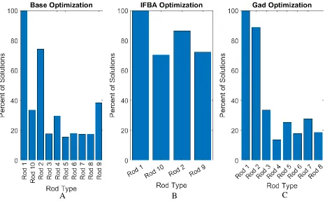
4.2 Burnable Poison Analysis Results
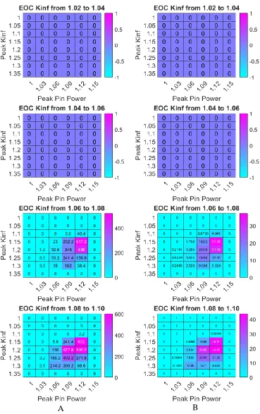
The number of generations for the runs of the IFBA only and gadolinium only cases are presented in Table 4-1. The average number of solutions per bin and associated error for the average value for the optimization using only IFBA and gadolinium as BP is presented in Figure 4-2. The average number of solutions per bin and associated error in the average number of solutions for the optimization using only IFBA for BP is presented in Figure 4-3. The average and error in counts per bin for the gadolinium only case are presented in Figure 4-4. Figure 4-5 shows the burnable
0.4 0.5 0.6 0.7 0.8 0.9 1 1.1 1.2 1.3 1.4
1.02 1.04 1.06 1.08 1.1 1.12 1.14 1.16
Ki
n
f
Peak Pin Power
Comparison of Pareto Front to Binned Solution Front
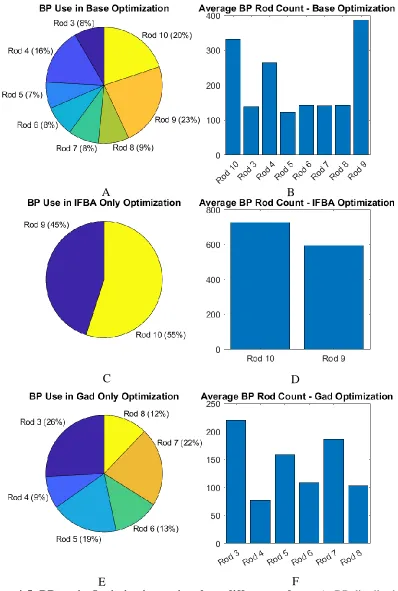
37 poison distribution for the base, IFBA only, and gadolinium only optimization cases, and the average number of burnable poison rods used in each optimization. Figure 4-6 shows the percentage of solutions that use each rod type.
Table 4-1: Number of Generations for Burnable Poison Analysis
Analysis Name Case Number
1 2 3 4 5 Average
Base 66 71 58 52 62 62
IFBA Only 62 54 62 59 61 60
Figure 4-2: Base Case Solution Space Results. A: Average number of solutions per bin in the solution space. B: Error in the average number of solutions per bin.
39
Figure 4-3: IFBA Only Solution Space Results. A: Average number of solutions per bin in the solution space. B: Error in the average number of solutions per bin.
Figure 4-4: Gadolinium Only Solution Space Results. A: Average number of solutions per bin in the solution space. B: Error in the average number of solutions per bin.
41
Figure 4-5: BP use in Optimizations using three different rod sets. A: BP distribution using IFBA and Gad. B: BP rod counts using IFBA and Gad. C: BP distribution using IFBA only. D: BP rod counts using IFBA only. E: BP distribution using Gad only. F: BP rod counts using Gad
only.
B A
D C
Figure 4-6: Average percentage of lattice solutions in final population using each rod type for the three rod set optimizations. A: IFBA and Gad rod set. B: IFBA Only rod set, C:
Gadolinium only rod set
It is interesting to note that when both IFBA and gadolinium are used as burnable poisons, the gadolinium rods are used in relatively even amounts. Rod 4 is used more than any other gadolinium rod though. When only gadolinium is allowed as the burnable poison however, there is a clear preference. Gadolinium rods with an accompanying uranium enrichment of 4.40% are used more often than rods with an enrichment of 4.95%. Additionally, rod 4 is the least used gadolinium rod.
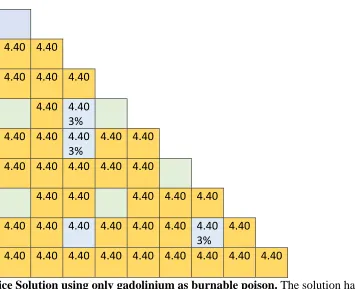
A solution containing both IFBA and gadolinium as the BP is presented in Figure 4-7. A solution containing only IFBA as the BP is presented in Figure 4-9. A solution containing only gadolinium as the BP is provided in Figure 4-10.
43
4.40 4.40
4.40 4.40 4.40 1% 4.40 4.95
IFBA
4.40 4.40 4.40 4.40 4.40
4.95 IFBA
4.40 4.40 4.40 4.40
4.40 4.40 4.40 4.95 IFBA
4.40
4.40 4.40 4.40 4.40 4.40 4.95 IFBA
4.40 4.40
4.40 4.40 IFBA
4.40 4.40 4.40 4.40 4.40 4.40 4.40
Figure 4-7: Lattice Solution combining IFBA and gadolinium as burnable poisons. The solution had a peak pin power of 1.132, peak kinf of 1.04483, and end kinf of 1.03618.
4.40 4.40 IFBA
4.40 4.40 4.40
4.40 4.40
4.40 4.40 4.40 IFBA
4.40 4.40
4.40 4.40 4.40 4.40 4.40
4.40 4.40 4.40 IFBA
4.95 4.40 IFBA 4.95
IFBA
4.40 4.40 4.40 4.40 4.95 IFBA
4.40 4.40
4.40 4.40 IFBA
4.40 4.40 4.40 4.40 4.40 4.40 4.40
Figure 4-8: Lattice Solution using only IFBA as burnable poison. The solution had a peak pin power of 1.108, peak kinf of 1.04773, and end kinf of 1.03935.
4.40 4.40
4.40 4.40 4.40
4.40 4.40 3% 4.40 4.40 4.40
3%
4.40 4.40
4.40 4.40 4.40 4.40 4.40
4.40 4.40 4.40 4.40 4.40
4.40 4.40 4.40 4.40 4.40 4.40 4.40 3%
4.40
4.40 4.40 4.40 4.40 4.40 4.40 4.40 4.40 4.40
Figure 4-9: Lattice Solution using only gadolinium as burnable poison. The solution had a peak pin power of 1.141, peak kinf of 1.15309, and end kinf of 1.15309.
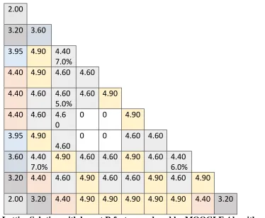
4.3 BOC BWR Problem
45
2.00 3.20 3.60 3.95 4.40 4.60 4.40 4.90 4.60 4.60 4.40 4.60 4.60 4.60 4.90 4.40 4.60 4.90 0 0 4.90 3.95 4.90 4.60 0 0 4.60 4.60 3.60 4.60 4.60 4.60 4.60 4.60 4.60 4.60 3.20 4.40 4.60 4.90 4.40 4.60 4.90 4.60 4.90 2.00 3.20 4.40 4.90 4.90 4.90 4.90 4.90 4.40 3.20
Figure 4-11: Lattice Solution with lowest R factor produced by MOOGLE Algorithm using 9 rod types for the BOC BWR optimization problem.
2.00
3.20 3.60
3.95 4.90 4.40 7.0%
4.40 4.90 4.60 4.60
4.40 4.60 4.60 5.0%
4.60 4.90
4.40 4.60 4.6 0
0 0 4.90
3.95 4.90 4.60
0 0 4.60 4.60
3.60 4.40 7.0%
4.90 4.60 4.60 4.90 4.60 4.40 6.0%
3.20 4.40 4.60 4.90 4.60 4.60 4.90 4.60 4.90
2.00 3.20 4.40 4.90 4.90 4.90 4.90 4.90 4.40 3.20
Figure 4-12: Lattice Solution with lowest R factor produced by MOOGLE Algorithm using 9 rod types at a BOC Kinf value near 1.20 for the BOC BWR optimization problem. Note: The first row indicates rod enrichment, the second row indicates rod gadolinium concentration.
Table 4-2: Minimum, Maximum, and Average Parameter Values for BOC BWR Optimization
Parameter Average Value Minimum Value Maximum Value
R factor 1.0485 0.9987 1.0917
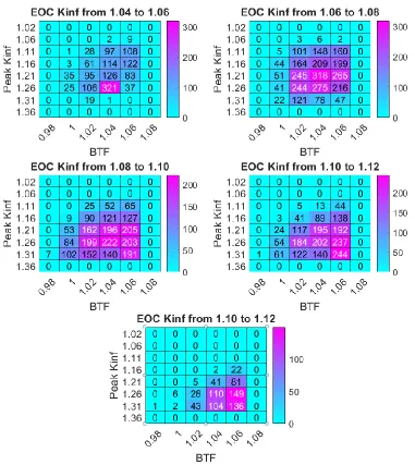
47 4.4 Depletion and Multiple Zone BWR Problem
The number of generations for the three different rod numbers used for the second BWR problem can be found in Table 4-3. The number of counts per bin for the eighteen-rod case are shown in Figure 4-13. The number of counts per bin for the fifteen-rod case are shown in Figure 4-14. The number of counts per bin for the twelve-rod case are shown in Figure 4-15. Average values for the optimization objectives are presented in
Table 4-4. Minimum values for the optimization objectives are presented in Table 4-5. Maximum values for the optimization objectives are given in Table 4-6.
Table 4-3: Number of Generations for the Second BWR Optimization Problem
Number of Rods Number of Generations
18 81
15 40
12 93
Table 4-4: Average Objective Values for the Second BWR Optimization Problem
Number of Rods BTF Peak Kinf EOC Kinf
18 1.063 1.239 1.091
15 1.065 1.226 1.077
Figure 4-13: Number of Counts per bin for the second BWR problem eighteen rod case. Table 4-5: Minimum Objective Values for the Second BWR Optimization Problem
Number of Rods BTF Peak Kinf EOC Kinf
18 1.012 1.086 1.051
15 1.021 1.093 1.053
12 1.013 1.087 1.050
Table 4-6: Maximum Objective Values for the Second BWR Optimization Problem
Number of Rods BTF Peak Kinf EOC Kinf
18 1.100 1.374 1.141
15 1.098 1.344 1.100
49
Figure 4-14: Number of counts per bin for the second BWR problem for the fifteen-rod case.
The breakdown of rod use is shown in Figures 4-16 and 4-17, and Table 4-7. Figure 4-16 and Table 4-7 shows how the percentage each rod type makes up in the optimization for the three different cases. Figure 4-17 shows the percentage of lattices containing each rod type. It is interesting to note that rods using gadolinium in the bottom axial zone are used in preference over rod types containing gadolinium in upper zones. The figures show that rods containing gadolinium in the lowest zone of the rod are used more than other rod types containing gadolinium.
Figure 4-16: Comparison of rod types used by the three different optimization cases for the second BWR optimization problem.
51 Table 4-7: Percentage of Rod Types Used in Second BWR Optimization
Rod Number
Percent of total rods used in Optimization
18 Rod Case 15 Rod Case 12 Rod Case
1 16 25 19
2 5 6 12
3 5 2 2
4 13 2 21
5 5 2 2
6 18 16 13
7 7 17 9
8 1 1 2
9 1 1 1
10 1 2 1
11 1 1 2
12 11 14 17
13 1 1
14 1 1
15 8 7
16 1
17 1
Chapter 5 Analysis of Results
Two methods are employed to compare different optimization cases to each other. The first method is epsilon indicator distance testing, in which an optimal solution front composed of the five base and test runs is compared to the ten individual optimizations. The second method compares the solution spaces explored by the test and base optimization cases.
5.1 Burnable Poison Analysis Discussion
Table 5-1 gives the average distances between the individual optimization runs of the base and test case and the optimal solution front composed of these cases. Figure 5-1 compares the solution front and solution spaces of the IFBA only test and base cases. Figure 5-2 compares the solution front and solution spaces of the gadolinium test and base cases. Figure 5-3 directly compares the solution fronts and solution spaces of the IFBA only, gadolinium only, and base case which used both gadolinium and IFBA as BP.
Table 5-1: Average Distance Comparison of IFBA and Gad Only
Case Name Case Part Average Distance for EOC Kinf Range
1.02 – 1.04 1.04 – 1.06 1.06 – 1.08 1.08 – 1.10 Total
IFBA
Test 2.69 8.88 14.31 67.80 93.67
Base 7.08 13.35 14.44 14.79 49.66
Difference -4.39 -4.48 -0.13 53.00 44.01
Gadolinium
Test NA NA 43.67 31.07 74.74
Base 3.78 9.73 14.62 14.61 42.74
Difference 3.78 9.73 29.05 16.45 32.00
![Figure 1-1: Fuel loading pattern for a nuclear reactor core [5].](https://thumb-us.123doks.com/thumbv2/123dok_us/1337605.1166741/16.612.173.467.128.388/figure-fuel-loading-pattern-nuclear-reactor-core.webp)