Abstract
Barlow, Gregory John. Design of Autonomous Navigation Controllers for Unmanned Aerial Vehicles Using Multi-objective Genetic Programming. (under the direction of Edward Grant.)
Unmanned aerial vehicles (UAVs) have become increasingly popular for many applications,
including search and rescue, surveillance, and electronic warfare, but almost all UAVs are
con-trolled remotely by humans. Methods of control must be developed before UAVs can become
truly autonomous. While the field of evolutionary robotics (ER) has made strides in using
evo-lutionary computation (EC) to develop controllers for wheeled mobile robots, little attention
has been paid to applying EC to UAV control. EC is an attractive method for developing UAV
controllers because it allows the human designer to specify the set of high level goals that are
to be solved by artificial evolution. In this research, autonomous navigation controllers were
developed using multi-objective genetic programming (GP) for fixed wing UAV applications.
Four behavioral fitness functions were derived from flight simulations. Multi-objective GP
used these fitness functions to evolve controllers that were able to locate an electromagnetic
energy source, to navigate the UAV to that source efficiently using on-board sensor
measure-ments, and to circle around the emitter. Controllers were evolved in simulation. To narrow the
gap between simulated and real controllers, the simulation environment employed noisy radar
signals and a sensor model with realistic inaccuracies. All computations were performed on a
92-processor Beowulf cluster parallel computer. To gauge the success of evolution, baseline
fitness values for a successful controller were established by selecting values for a minimally
successful controller. Two sets of experiments were performed, the first evolving controllers
directly from random initial populations, the second using incremental evolution. In each set
of experiments, autonomous navigation controllers were evolved for a variety of radar types.
Both the direct evolution and incremental evolution experiments were able to evolve controllers
incremental evolution over direct evolution. The final incremental evolution experiment on the
most complex radar investigated in this research evolved controllers that were able to handle all
of the radar types. Evolved UAV controllers were successfully transferred to a wheeled mobile
robot. An acoustic array on-board the mobile robot replaced the radar sensor, and a speaker
emitting a tone was used as the target. Using the evolved navigation controllers, the mobile
robot moved to the speaker and circled around it. Future research will include testing the best
DESIGN OF AUTONOMOUS NAVIGATION CONTROLLERS
FOR UNMANNED AERIAL VEHICLES USING
MULTI-OBJECTIVE GENETIC PROGRAMMING
BY
GREGORY J. BARLOW
A THESIS SUBMITTED TO THE GRADUATE FACULTY OF NORTH CAROLINA STATE UNIVERSITY
IN PARTIAL FULFILLMENT OF THE REQUIREMENTS FOR THE DEGREE OF
MASTER OF SCIENCE
ELECTRICAL AND COMPUTER ENGINEERING
RALEIGH
MARCH 2004
Dedicated to
Biography
Gregory John Barlow was born June 14, 1980 in Greensboro, North Carolina to John Black
Barlow, Jr. and Cheryl Stevens Barlow. He graduated from the North Carolina School of
Sci-ence and Mathematics, Durham, North Carolina in May 1999. He received Bachelor of SciSci-ence
degrees in Electrical Engineering and Computer Engineering from North Carolina State
Uni-versity, Raleigh, North Carolina in May 2003. He received the Master of Science Degree in
Electrical Engineering from North Carolina State University, Raleigh, North Carolina in May
2004.
As an undergraduate, Gregory was a Barry M. Goldwater Scholar, a John T. Caldwell Scholar,
a Caldwell Fellow, and a University Scholar. He received a North Carolina State University
Undergraduate Research Award for the spring of 2001, a National Science Foundation Summer
Undergraduate Fellowship in Sensor Technologies at the University of Pennsylvania for the
summer of 2001, and was a winner of the 2001 North Carolina State University Undergraduate
Research Symposium and the 2001 Sigma Xi Student Research Symposium.
Gregory is a member of Eta Kappa Nu Electrical and Computer Engineering Honor Society,
Tau Beta Pi Engineering Honor Society, the Honor Society of Phi Kappa Phi, the Institute of
Electrical and Electronics Engineers, and the International Society for Genetic and
Acknowledgments
I would like to thank the members of my committee, Dr. Edward Grant, Dr. Choong K. Oh,
Dr. Mark W. White, and Dr. H. Troy Nagle. I would like to thank Dr. Edward Grant for all of
his support and encouragement. In all the years I’ve been privileged to work with him, he has
given me so many opportunities to learn and grow. Dr. Grant has helped me to become a better
researcher and a better person. I would also like to especially thank Dr. Choong Oh for giving
me the opportunity to become involved in this research. Dr. Oh has been a wonderful mentor.
I would like to acknowledge the financial support of this work provided by the Office of Naval
Research (ONR) through the United States Naval Research Laboratory (NRL) under Dr.
Mari-bel Soto (ONR) and Dr. Choong Oh (NRL). Computer time on the 92 processor Beowulf
cluster was furnished by NRL (Code 5732).
I would like to thank all the members of the Center of Robotics and Intelligent Machines
(CRIM), past and present, for their collaboration and support. I have spent six wonderful years
in the CRIM and have had the chance to work with many great people. I would especially like
to thank Andrew Nelson, John Galeotti, Leonardo Mattos, and Marc Edwards.
Most of all, I would like to thank my parents, John and Cheryl Barlow. Their persistent and
wholehearted commitment to my education and growth as a person have made me what I am
today. I am forever grateful. I would also like to thank my three sisters, Logan, Lindsey, and
Contents
List of Figures ix
List of Tables xiii
List of Abbreviations xv
1 Introduction 1
1.1 Motivation and Research Goals . . . 1
1.2 Overview of Thesis Chapters . . . 2
2 Literature Review 4 2.1 Evolutionary Robotics . . . 5
2.1.1 History of Evolutionary Robotics Research . . . 6
2.1.2 Evolutionary Robotics Controller Architectures . . . 8
2.1.3 Simulation . . . 9
2.1.4 Robot Types . . . 10
2.2 Genetic Programming . . . 11
2.2.1 Evolutionary Process . . . 12
2.2.2 Concerns and Strategies . . . 13
2.3.1 Functional Fitness Functions . . . 16
2.3.2 Aggregate Fitness Functions . . . 17
2.3.3 Competitive Fitness Evaluation . . . 18
2.3.4 Multi-objective Optimization . . . 19
2.3.5 Incremental Evolution . . . 21
3 Unmanned Aerial Vehicle Control 25 3.1 Simulation Environment . . . 26
3.2 Unmanned Aerial Vehicles . . . 27
3.2.1 Characteristics . . . 28
3.2.2 Applications . . . 30
3.2.3 Operation . . . 32
3.2.4 Controller Architecture . . . 33
3.2.5 Simulation Flight Model . . . 33
3.3 Radar . . . 34
3.3.1 Radar Types . . . 34
3.3.2 Radar Modeling . . . 35
3.4 Sensors . . . 36
3.5 Problem Difficulty . . . 37
3.6 Transference to real UAVs . . . 38
4 Evolution and Fitness Evaluation 40 4.1 Multi-objective Genetic Programming . . . 42
4.1.1 Genetic Programming Parameters . . . 42
4.1.2 Functions and Terminals . . . 47
4.2 Fitness Functions . . . 50
4.2.1 Normalized distance . . . 51
4.2.2 Circling distance . . . 52
4.2.3 Level time . . . 53
4.2.4 Turn cost . . . 54
4.2.5 Combining the Fitness Measures . . . 55
4.3 Incremental Evolution . . . 56
4.3.1 Functional Incremental Evolution . . . 57
4.3.2 Environmental Incremental Evolution . . . 58
5 Experiments and Results 60 5.1 Effectiveness of Fitness Functions . . . 61
5.2 Metrics for Post-evolution Controller Evaluation . . . 63
5.3 Direct Evolution . . . 65
5.3.1 Continuously Emitting, Stationary Radar . . . 65
5.3.2 Intermittently Emitting, Stationary Radar with Regular Period . . . 70
5.3.3 Intermittently Emitting, Stationary Radar with Irregular Period . . . 78
5.3.4 Continuously Emitting, Mobile Radar . . . 86
5.3.5 Intermittently Emitting, Mobile Radar with Regular Period . . . 94
5.4 Incremental Evolution . . . 102
5.4.1 Seed Populations . . . 102
5.4.2 Intermittently Emitting, Stationary Radar . . . 103
5.4.3 Continuously Emitting, Mobile Radar . . . 106
5.4.4 Intermittently Emitting, Stationary Radar with Multiple Increments . . 108
5.4.5 Intermittently Emitting, Mobile Radar with Multiple Increments . . . . 111
5.4.6 Analysis of Incrementally Evolved Controllers . . . 112
6 Conclusion and Future Research 125
6.1 Conclusions . . . 125
6.2 Future Research . . . 128
7 References 129 Appendices 135 A Experimental Results 136 A.1 Direct Evolution . . . 136
A.1.1 Continuously Emitting, Stationary Radar . . . 136
A.1.2 Intermittently Emitting, Stationary Radar with Regular Period . . . 137
A.1.3 Intermittently Emitting, Stationary Radar with Irregular Period . . . 138
A.1.4 Continuously Emitting, Mobile Radar . . . 139
A.1.5 Intermittently Emitting, Mobile Radar with Regular Period . . . 140
A.2 Incremental Evolution . . . 141
A.2.1 Seed Population . . . 141
A.2.2 Intermittently Emitting, Stationary Radar . . . 142
A.2.3 Continuously Emitting, Mobile Radar . . . 143
A.2.4 Intermittently Emitting, Stationary Radar with Multiple Increments . . 144
A.2.5 Intermittently Emitting, Mobile Radar with Multiple Increments . . . . 145
B Sample Results from Evolutionary Runs 147 B.1 Continuously Emitting, Stationary Radar . . . 147
List of Figures
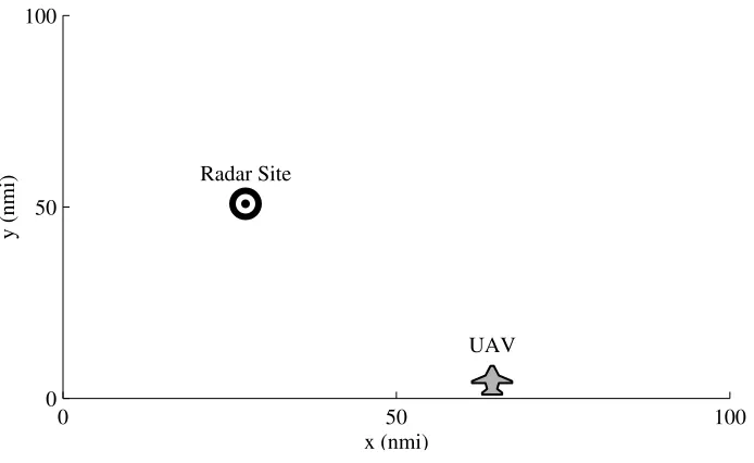
3.1 The simulation area, as shown, is 100 nmi by 100 nmi. The UAV is placed randomly along the southern edge of the simulation area, and the radar is placed randomly anywhere within the environment. . . 27
3.2 The Predator medium altitude long endurance unmanned aerial vehicle. . . 28
3.3 The Dakota unmanned aerial vehicle. . . 29
3.4 The angle of arrival (AoA) is the angle between the UAV heading and the incoming signal. . . 37
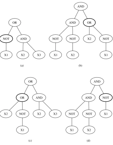
4.1 An example of the recombination process, with the crossover points high-lighted. Two parent program trees (a and b) produce two children (c and d). . . 45
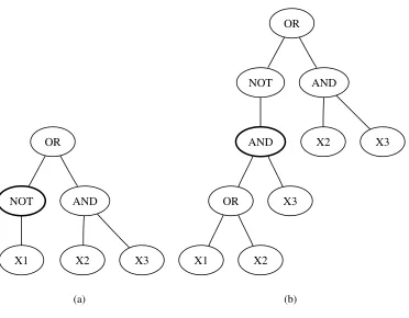
4.2 An example of the mutation process, with the mutation point highlighted. A parent tree (a) produces a mutated child tree (b). . . 46
5.1 Histogram of the number of successful controllers for each evolutionary run for continuously emitting, stationary radars. . . 67
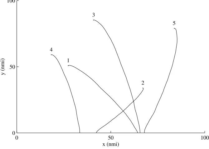
5.2 Five sample flight paths for an evolved controller flying a UAV to continuously emitting, stationary radars. . . 67
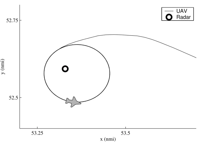
5.3 A sample flight path for a UAV guided by an evolved controller flying to a continuously emitting, stationary radar. . . 69
5.4 A closeup of the UAV flight path shown in Figure 5.3 after 43 minutes and 20 seconds. The UAV has just begun to circle around the radar. . . 69
5.5 A closeup of the UAV flight path shown in Figure 5.3 after 47 minutes and 5 seconds. The UAV is circling around the radar. . . 70
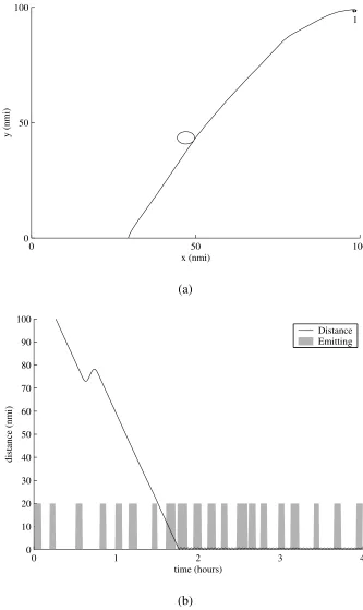
5.7 Flight path 1 for a UAV controller to an intermittently emitting, stationary radar (a), the distance between the UAV and the radar, and the emitting period and duration of the radar (b). . . 73
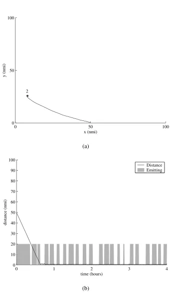
5.8 Flight path 2 for a UAV controller to an intermittently emitting, stationary radar (a), the distance between the UAV and the radar, and the emitting period and duration of the radar (b). . . 74
5.9 Flight path 3 for a UAV controller to an intermittently emitting, stationary radar (a), the distance between the UAV and the radar, and the emitting period and duration of the radar (b). . . 75
5.10 Flight path 4 for a UAV controller to an intermittently emitting, stationary radar (a), the distance between the UAV and the radar, and the emitting period and duration of the radar (b). . . 76
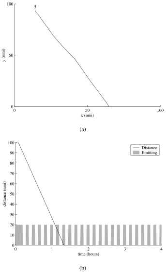
5.11 Flight path 5 for a UAV controller to an intermittently emitting, stationary radar (a), the distance between the UAV and the radar, and the emitting period and duration of the radar (b). . . 77
5.12 Histogram of the number of successful controllers for each evolutionary run for intermittently emitting, stationary radars with an irregular period. . . 80
5.13 Flight path 1 for a UAV controller to an intermittently emitting, stationary radar with an irregular period (a), the distance between the UAV and the radar, and the emitting period and duration of the radar (b). . . 81
5.14 Flight path 2 for a UAV controller to an intermittently emitting, stationary radar with an irregular period (a), the distance between the UAV and the radar, and the emitting period and duration of the radar (b). . . 82
5.15 Flight path 3 for a UAV controller to an intermittently emitting, stationary radar with an irregular period (a), the distance between the UAV and the radar, and the emitting period and duration of the radar (b). . . 83
5.16 Flight path 4 for a UAV controller to an intermittently emitting, stationary radar with an irregular period (a), the distance between the UAV and the radar, and the emitting period and duration of the radar (b). . . 84
5.17 Flight path 5 for a UAV controller to an intermittently emitting, stationary radar with an irregular period (a), the distance between the UAV and the radar, and the emitting period and duration of the radar (b). . . 85
5.19 Flight path 1 for a UAV controller to a continuously emitting, mobile radar (a), the distance between the UAV and the radar, and the emitting period and duration of the radar (b). . . 89
5.20 Flight path 2 for a UAV controller to a continuously emitting, mobile radar (a), the distance between the UAV and the radar, and the emitting period and duration of the radar (b). . . 90
5.21 Flight path 3 for a UAV controller to a continuously emitting, mobile radar (a), the distance between the UAV and the radar, and the emitting period and duration of the radar (b). . . 91
5.22 Flight path 4 for a UAV controller to a continuously emitting, mobile radar (a), the distance between the UAV and the radar, and the emitting period and duration of the radar (b). . . 92
5.23 Flight path 5 for a UAV controller to a continuously emitting, mobile radar (a), the distance between the UAV and the radar, and the emitting period and duration of the radar (b). . . 93
5.24 Histogram of the number of successful controllers for each evolutionary run for intermittently emitting, mobile radars. . . 96
5.25 Flight path 1 for a UAV controller to an intermittently emitting, mobile radar (a), the distance between the UAV and the radar, and the emitting period and duration of the radar (b). . . 97
5.26 Flight path 2 for a UAV controller to an intermittently emitting, mobile radar (a), the distance between the UAV and the radar, and the emitting period and duration of the radar (b). . . 98
5.27 Flight path 3 for a UAV controller to an intermittently emitting, mobile radar (a), the distance between the UAV and the radar, and the emitting period and duration of the radar (b). . . 99
5.28 Flight path 4 for a UAV controller to an intermittently emitting, mobile radar (a), the distance between the UAV and the radar, and the emitting period and duration of the radar (b). . . 100
5.29 Flight path 5 for a UAV controller to an intermittently emitting, mobile radar (a), the distance between the UAV and the radar, and the emitting period and duration of the radar (b). . . 101
5.31 Evolutionary process for incremental evolution of controllers for intermittently emitting, stationary radars. . . 105
5.32 Histogram of the number of successful controllers incrementally evolved on intermittently emitting, stationary radars. . . 106
5.33 Evolutionary process for incremental evolution of controllers for continuously emitting, mobile radars. . . 107
5.34 Histogram of the number of successful controllers incrementally evolved on continuously emitting, mobile radars. . . 108
5.35 Evolutionary process for the incremental evolution of controllers for intermit-tently emitting, stationary radars using multiple increments. . . 110
5.36 Histogram of the number of successful controllers incrementally evolved on intermittently emitting, stationary radars over multiple increments. . . 111
5.37 Evolutionary process for the incremental evolution of controllers for intermit-tently emitting, mobile radars using multiple increments. . . 113
5.38 Histogram of the number of successful controllers incrementally evolved on intermittently emitting, mobile radars over multiple increments. . . 114
5.39 Depth by generation in the incremental evolution of controllers for intermit-tently emitting, mobile radars. Transitions between the stages of evolution are shown. . . 115
5.40 Complexity by generation in the incremental evolution of controllers for inter-mittently emitting, mobile radars. Transitions between the stages of evolution are shown. . . 115
5.41 EvBot II, a small, wheeled mobile robot. . . 118
5.42 Flight paths for a UAV controller to a continuously emitting, stationary radar using a sensor accurate within (a)±10◦and (b)±45◦. . . 120
5.43 Flight path in simulation for Controller 1 to a continuously emitting, stationary radar using a sensor accurate within±45◦. . . 121
5.44 Path for an EvBot running Controller 1 moving to a continuously emitting, stationary speaker using a real acoustic array sensor. . . 122
5.45 Flight path in simulation for Controller 2 to a continuously emitting, stationary radar using a sensor accurate within±45◦. . . 123
List of Tables
4.1 Genetic programming parameters . . . 43
5.1 Baseline values used to measure the performance of evolution. . . 64
5.2 Results for experiments with continuously emitting, stationary radars. . . 66
5.3 Fitness values for five UAV flight paths to continuously emitting, stationary radars shown in Figure 5.2. . . 68
5.4 Fitness values for the flight path examined in Figures 5.3, 5.4, and 5.5. . . 68
5.5 Results for experiments with intermittently emitting, stationary radars with reg-ular periods. . . 71
5.6 Fitness values for five UAV flight paths to intermittently emitting, stationary radars shown in Figures 5.7, 5.8, 5.9, 5.10, and 5.11. . . 72
5.7 Results for experiments with intermittently emitting, stationary radars with ir-regular periods. . . 79
5.8 Fitness values for five UAV flight paths to intermittently emitting, stationary radars with irregular periods shown in Figures 5.13, 5.14, 5.15, 5.16, and 5.17. . 80
5.9 Results for experiments with continuously emitting, mobile radars. . . 87
5.10 Fitness values for five UAV flight paths to continuously emitting, mobile radars shown in Figures 5.19, 5.20, 5.21, 5.22, and 5.23. . . 94
5.11 Results for experiments with intermittently emitting, mobile radars. . . 95
5.12 Fitness values for five UAV flight paths to intermittently emitting, mobile radars shown in Figures 5.25, 5.26, 5.27, 5.28, and 5.29. . . 95
5.14 Results for incremental evolution experiments evolved on intermittently emit-ting, stationary radars. . . 105
5.15 Results for incremental evolution experiments evolved on continuously emit-ting, mobile radars. . . 107
5.16 Results for incremental evolution experiments evolved on intermittently emit-ting, stationary radars evolved in multiple increments. . . 109
5.17 Results for incremental evolution experiments evolved on intermittently emit-ting, mobile radars evolved in multiple increments. . . 112
List of Abbreviations
AI Artificial Intelligence
AL Artificial Life
ANN Artificial Neural Networks
AoA Angle of Arrival
EA Evolutionary Algorithm
EC Evolutionary Computation
ER Evolutionary Robotics
EW Early Warning (Radar)
GA Genetic Algorithm
GP Genetic Programming
GPS Global positioning system
nmi Nautical Miles
RC Remote Control
TA Target Acquisition (Radar)
TT Target Tracking (Radar)
Chapter 1
Introduction
1.1
Motivation and Research Goals
Unmanned aerial vehicles (UAVs) have become increasingly popular for many applications,
including search and rescue, surveillance, and electronic warfare, but almost all UAVs are
controlled remotely by humans. For UAVs to become truly useful, especially for military
ap-plications, methods of autonomous control must be developed. While the field of evolutionary
robotics (ER) has made strides in using artificial evolution to develop controllers for wheeled
mobile robots, little attention has been paid to controlling UAVs. Evolutionary computation
(EC) is an attractive method for developing UAV control because it allows the human designer
to specify a set of high level goals to be solved by artificial evolution.
This research presents an approach to designing behavioral navigation controllers for fixed
wing UAVs. Multi-objective genetic programming (GP) was used to evolve these controllers
in simulation. The goal of the research was to produce controllers that could locate an
electro-magnetic energy source – a radar in this research – navigate the UAV to the source efficiently,
UAV flight tests, were established to measure these behaviors: the average normalized
dis-tance to the radar, the circling disdis-tance, the amount of time spent flying with a roll angle of
0◦, and a measure of the cost of turning sharply. These fitness functions were combined using
multi-objective optimization. Research began by examining a very simple radar type that was
continuously emitting and stationary. Experiments progressed to more difficult radar types,
including radars that emitted intermittently and radars that moved around the simulation area.
A second set of experiments used incremental evolution to improve the chance of evolving
successful controllers.
While there has been some success in evolving controllers directly on real robots,
simula-tion is much more common. For UAVs, simulasimula-tion is the only feasible method for evolving
controllers. A UAV cannot be operated for long enough to evolve a sufficiently competent
controller, the use of an unfit controller could result in damage to the aircraft, and flight tests
are very expensive. The development of the simulation environment is extremely important to
the future success of evolved controllers. After being evolved in simulation, controllers must
be transfered to real UAVs, and ensuring that the evolved controllers are sufficiently robust
was an important consideration of the evolutionary process. Methods for effective transference
were incorporated into the simulation by abstracting navigation control from UAV flight, tuning
simulation parameters for equivalence to real aircraft, and adding noise to the simulation.
1.2
Overview of Thesis Chapters
Chapter 2 reviews literature related to the research, including the areas of evolutionary
com-putation, genetic programming, and evolutionary robotics. Methods for measuring fitness in
evolutionary robotics are also examined. Issues within the literature of particular concern to
Chapter 3 describes the problem of controlling UAVs to locate radars. Considerations and
cur-rent trends in UAV technology are examined. The simulation environment, including models
for UAVs, radar sites, and sensors, is presented. The difficulty of the problem and the issue of
transference are discussed.
Chapter 4 presents the multi-objective GP algorithm used to evolve controllers. Four fitness
measures were designed to promote the evolution of good behaviors: normalized distance,
cir-cling distance, level time, and turn cost. The fitness functions and strategies used to evolve
controllers are presented along with the parameters used by GP. Methods of incremental
evo-lution used to evolve controllers are also presented.
Chapter 5 describes the use of multi-objective GP to evolve controllers for a variety of radar
types. First, the effectiveness of the four fitness functions in producing controllers that satisfy
the mission goals is analyzed. After presenting a post-evolution metric for performance
eval-uation, experimental results for controllers evolved on a variety of radar types are presented.
Results are presented for experiments using both direct and incremental evolution. Finally, the
transference of evolved controllers to real robots is described.
Chapter 6 presents concluding remarks on the success of the research. An overview of future
Chapter 2
Literature Review
To be truly helpful to humans, robots must be intelligent and able to function autonomously. To
be considered intelligent, a robot must not perform tasks mindlessly, and to be considered truly
autonomous, a robot must be able to function in a complex and noisy environment without
human aid [55]. However, most of the robots known to the general public, including Honda’s
ASIMO humanoid robot, robots shown on television, and most industrial robots, lack both
autonomy and intelligence. Instead, they are either directly controlled by humans or
prepro-grammed, often operating in a simplified environment. Robots have the potential to improve
our lives in many ways, performing difficult, dangerous, and repetitive tasks, but to make this
truly possible, robots must be intelligent and autonomous.
Since neurophysiologist W. Grey Walter designedMachina speculatrixin the early 1950’s [77], the area of autonomous robots has been an active area of research. The Machina speculatrix, a robot which Walter also called a tortoise, was a three-wheeled robot with a brain composed
of only a few analog neurons. The tortoise displayed simple behaviors including returning to a
recharging station when its battery was low and homing on a light source. Walter showed how
environment.
As the field of artificial intelligence (AI) grew, so did research on autonomous robotics. The
dominant controller architecture used for autonomous agents was the classical [70] or
hierar-chical [55] architecture. In this architecture, the robot senses the world, plans the next action,
and then acts. An internal global world model is maintained to be used by the planner. The
planning stage might take a long time, and changes in the environment might be ignored. The
earliest example of a robot using this architecture is Shakey [61], a robot designed at the
Stan-ford Research Institute. Shakey used the STRIPS algorithm to generate plans.
In the mid-1980’s, Brooks suggested an alternative to the classical architecture [7], which he
would later call the subsumption architecture [8]. In the subsumption architecture, sensing and
action are tightly linked, and the world is used as its own model [9]. This research has expanded
into the field of behavior-based robotics [3]. Behavior-based robotics differs from the classical
architecture in the diminished importance of planning. While some behavioral architectures
still use planning, there is a much tighter reactive linking between sensing and action than in
the hierarchical architecture [55]. Behavioral architectures that are completely reactive, with
no planning at all, are called “model-free” controllers. Model-free controllers have no internal
environmental model, and effector outputs are a direct function of sensor inputs [35].
2.1
Evolutionary Robotics
The field of evolutionary robotics (ER) [62] combines research on evolutionary computation
(EC) [5,31] with behavior-based robotics and artificial life (AL) [1]. The primary goal of ER is
the automatic design of behavioral controllers with no internal environmental model. ER uses
a population-based evolutionary algorithm to evolve autonomous robot controllers for a target
Many evolved robot controllers are model-free. It is possible to include explicit environmental
models for use by evolved controllers [35], but most research does not. While it is feasible
for evolution to produce internal world models, most environments investigated in ER are not
sufficiently inaccessible to require it. The evolution of internal models is also unlikely using
current ER techniques.
2.1.1
History of Evolutionary Robotics Research
Some of the earliest experimental ER work was done by Koza [40]. He used genetic
program-ming (GP) [39] to evolve a subsumption controller for the wall-following problem approached
by Mataric in [52]. The program evolved by Koza was similar in size to the subsumption
pro-grams written by Mataric. While the program evolved by GP was intended to control a real
robot, tests were done only in simulation, making it difficult to gauge the true effectiveness of
the evolved controller.
The research group at the University of Sussex [12] applied the term “evolutionary robotics” to
this field in 1993. Much of the early ER work was done by the Sussex group [12, 28, 29, 33] or
the collaboration between Stephano Nolfi, Dario Floreano, and others [21, 50, 62, 64]. Reviews
of the field of ER at various stages can be found in [29, 51, 57, 62].
Much of the early ER research studied obstacle avoidance navigation, and the evolution of this
type of behaviors continues in current research. Nolfi, Floreano, Miglino, and Mondada [64]
evolved navigation and obstacle avoidance on a real robot that used 8 infrared (IR) sensors
and was controlled by an artificial neural network (ANN). Successful behaviors were produced
after 100 generations, which took about 60 hours, since evolution was embodied on actual
robots. Jakobi, Husbands, and Harvey [33] evolved obstacle-avoiding behaviors in a simulated
Edner [16] evolved a GP controller for obstacle avoidance, first in simulation and then on a
real robot. Filliat, Kodjabachian, and Meyer [19] evolved obstacle avoidance in a six-legged
walking robot. In their research, the ANN controller was evolved in simulation, and then the
final controller was successfully tested on a real robot.
Homing is another common behavior studied in ER research. Floreano and Mondada [21]
evolved a neural network controller that could locate and periodically return to a battery charger
when energy levels got low. Evolution took place entirely on real robots. Lund and Hallam [47]
evolved a controller for a similar task, but evolution took place in simulation. They tested the
evolved ANN on a real robot, with behavior similar to simulation.
Another problem often studied in ER research is object movement. Lee, Hallam, and Lund
[43] evolved a GP controller to solve a box-pushing problem. The controller was evolved
in simulation and then transferred to real robots. Results showed that the evolved controller
was very capable at the task and there was no loss of performance when the controller was
transferred to a real robot. Kamio, Misuhashi, and Iba [34] evolved a GP controller for a
walking robot to push a box to a goal. The controller was evolved in simulation, and then
transferred to a real robot, where the controller was refined using Q-learning. Liu and Iba [44]
evolved GP controllers for two robots, one serving as a “hand”, the other as an “eye”. The
controller was evolved in simulation to carry an object to a goal. The controllers have been
transferred to real robots, but results on the success of transference are not yet available.
Another class of problems that has been studied in ER is game playing. Evolving robots to
play games can be more difficult than evolving simple behaviors, since successful strategies for
playing games may require multiple behaviors. Hsu and Gustafson [32] evolved agents to play
keep-away soccer. Their GP controllers were not tested on real robots. Nelson et al. [57–60]
evolved ANN controllers to play capture the flag. Evolved controllers were competitive with
In many of these experiments, the problems to be solved were designed specifically for
re-search purposes. While simple problems generally require a small number of behaviors, more
complex real-world problems might require the coordination of multiple behaviors in order to
achieve the goals of the problem. Very little of the ER work to date has been intended for use
in real-life applications.
2.1.2
Evolutionary Robotics Controller Architectures
A variety of controller architectures have been used in ER. The subsumption architecture was
used by Koza [40] early in ER research, and continues to be used today by some researchers
[44]. Genetic algorithms have been used to evolve rule sets for control [49, 79]. The use of
evolvable hardware for robot control has also been studied [35]. The two most popular control
architectures, however, are artificial neural networks and genetic programming.
ANNs consist of many simple processing units, or neurons, with many interconnections [20].
ANNs are the most popular controller structure used in ER research [12, 19, 21, 28, 29, 33, 47,
50, 57–60, 62, 64]. To speed up evolution, many studies restrict the complexity of network
topologies [21]. In some studies, the network topology is allowed to evolve along with the
weights [45, 54, 57], vastly increasing the search space, but making the use of ANNs more
scalable to difficult problems.
Despite Koza’s early ER work with GP, ANNs have dominated ER research. However, GP
has also been shown to produce functional behaviors for autonomous robot control [16, 32,
34, 43, 44, 65]. While ANNs only require the designer to specify constraints on the network
topology, GP requires additional human involvement prior to evolution. The designer must
specify the functions available to evolution, a process which does introduce human bias into
GP is often not such a disadvantage; the natural constraints of the problem often make function
selection more obvious.
2.1.3
Simulation
Early in ER research, Brooks noted that the evolution of robot controllers would probably
need to occur in simulation [10]. While some controllers have been evolvedin situ on phys-ical robots, evolution requires many evaluations to produce good behaviors, which generally
takes an excessive amount of time on real robots. Evolving controllers in simulation is less
constraining, because evaluations are much faster and can be parallelized. Since simulation
environments cannot be perfectly equivalent to the conditions a real robot would face,
transfer-ence of controllers evolved in simulation to real robots has been an important issue.
Early in ER research, many studies evolved controllers directly on physical robots [21, 62, 64].
Though the availability of computational power has made simulation increasingly attractive,
some research using embodied evolution continues [16, 50]. Embodied evolution is often
preferable to evolution using simulation because a model of the world doesn’t need to be
cre-ated for simulation. Embodied evolution can directly test the performance of controllers on the
exact problems one is interested in solving, including the noise from the actual environment.
However, embodied evolution is very slow, which constrains the complexity of problems that
can be solved in a reasonable amount of time.
Simulation has been used since the beginning of ER research [40] with varying success for the
control of real robots. Some simulated controllers are never tested on actual robots, and some
fail to transfer well. However, many controllers evolved in simulation have been successfully
transferred to real robots [19, 29, 33, 34, 43, 47, 57, 59, 60]. Adding noise to the simulation is
one method that has proved successful in evolving controllers that transfer well to real robots.
2.1.4
Robot Types
A variety of robot types have been used in ER research. By far the most common are wheeled
mobile robot experiments [16, 21, 29, 33, 35, 43, 44, 47, 50, 57–60, 62, 64]. The most popular
wheeled robot in use for ER research has been the Khepera [21, 29, 33, 43, 44, 47, 62, 64]. Some
researchers using the Khepera have now begun using a larger robot by the same manufacturer
called the Koala [50]. Other research has used existing wheeled research robots [16, 35]. At
North Carolina State University, the EvBot [24] and EvBot II [53] mobile robots have been
designed specifically for ER research [57–60].
ER research has extended to other robot types as well. Some researchers have done ER
exper-iments with walking robots. Filliat et al. [19] evolved locomotion and obstacle avoidance for
a walking robot with six legs. Kamio et al. [34] evolved a controller for a Sony AIBO
four-legged walking robot. The goal of this robot was to solve a box pushing task. At the University
of Sussex, Harvey, Husbands, Cliff, Thompson, and Jakobi [28, 29] used a specialized gantry
robot to do ER research. This robot was composed of a camera assembly suspended from a
gantry. The camera was aimed at a mirror angled at 45◦ so the camera could see in a way
similar to a camera mounted on a wheeled mobile robot. The mirror could be rotated to change
the “direction” this robot was facing. The gantry enabled the camera mechanism to be moved
within a plane. This gantry robot could be used much like a wheeled mobile robot. A variety
of ER experiments including vision work were done with this robot.
A robot type that has received relatively little attention has been the unmanned aerial vehicle
(UAV). ER experiments on flying vehicles can be separated into two general classes of aircraft:
fixed wing and rotary wing. The most common type, especially for military applications, is the
fixed wing UAV [14]. Hoffmann, Koo, and Shakernia [30] evolved a rotary wing helicopter
autopilot using evolutionary strategies to evolve a fuzzy logic rule base. Shim, Koo, Hoffmann,
tracking control in simulation. They showed that the evolved controller was able to handle
un-certainties and disturbances. Marin, Radtke, Innis, Barr, and Schultz [49] evolved a controller
for a UAV of an unspecified type. They evolved a set of rules to reactively control a UAV’s
flight based on target detection. Their experiments were only in simulation, the movement of
the UAV was grid-based, and the UAV could move in any direction at every time step.
Be-cause of the unrealistic nature of the simulation, it would have be difficult to control real UAVs
with the evolved controllers. In related work, Wu, Schultz, and Agah [79] evolved a control
scheme for micro air vehicles. Their evolved control system was distributed. Each vehicle had
its own controller, though all controllers were identical. Rule sets were evolved to control the
UAVs. Like the experiments in [49], only simulation was used, simulation was unrealistic, and
no testing on real UAVs was attempted. Meyer, Doncieux, Filliat, and Guillot [54] evolved a
neural network control system for a simulated blimp. Unlike rotary wing and fixed wing UAVs,
a blimp is very stable and easy to pilot. The goal of the research was to develop controllers
capable of countering wind to maintain a constant flying speed. The evolved control system
was only tested in simulation.
2.2
Genetic Programming
Genetic programming (GP) is a subfield of evolutionary computation (EC) [5] that uses a
ge-netic algorithm (GA) to evolve computer programs. EC uses a computer model of the naturally
occurring evolutionary process to solve problems [31]. A GA, a type of EC algorithm,
oper-ates on a population of individual objects, each with its own fitness, using genetic operators
like recombination and mutation to create a new generation. As this process is repeated, the
principle of survival of the fittest improves the fitness of the population.
GP uses a GA to evolve populations of computer programs. The GP paradigm was introduced
is much more effective [39]. GP allows for individuals to vary in size, which is necessary for
computer programs of varying lengths. Like most subfields of EC, GP is domain-independent.
GP has been applied to a diverse selection of problems. Extensive information on GP is
avail-able in Koza’s books [36–38].
2.2.1
Evolutionary Process
GP represents an individual as a tree, where each node represents a programming command.
Each non-leaf node is a function, which takes at least one argument, and each leaf node is a
terminal, which takes no arguments. A GP program tree can also be seen as an S-expression
similar to those in LISP, though GP systems are written in many languages.
The most common method for evolving computer programs using GP is generational evolution.
First, an initial population of random computer programs is generated. This population can be
generated in several ways, including setting the initial depth of all individuals to be the same,
ramping the initial depth of individuals over the population, or mixing these methods. After
the initial population has been created, evolution begins. During each generation, GP evaluates
each individual in the population and assigns it a fitness value using a fitness function. Then, a
new generation is formed by probabilistically selecting one or more parent programs from the
population and applying genetic operators to them. Three genetic operators are typically used,
and the percentage of time each is applied is set as a parameter of evolution. Reproduction
directly copies a selected individual to the new population. Crossover recombines two parent
programs to create new children. Mutation creates one new individual by mutating a single
parent. Mutation is typically done by selecting a node within the tree, destroying the subtree
below that point, and creating a new random subtree in its place. The mutation rate, the
per-centage of the time that mutation is applied, is usually set to be very small for GP, as mutation
being stuck in local minima. Evolution takes place over a specified number of generations
or until a success criterion is satisfied. Koza [36–38] provides extensive information on the
specific implementation of GP in software.
2.2.2
Concerns and Strategies
While the general framework of GP is well defined, many parameters of the algorithm can be
altered. There have been large numbers of studies investigating all aspects of GP in the hope
of making the evolutionary process efficient and successful. Two important parameters for
controlling GP are the population size and the maximum number of generations. Crossover
benefits from a large population, though too large a population can make propagation of good
behaviors difficult. Another parameter for controlling evolution is the ratio between crossover
and mutation operations. Typically, GP uses the crossover operation more than 90 percent of
the time. Evolution can also be controlled by varying the crossover and selection types [38].
The evaluation method is also important to the success of GP. Panait and Luke [67] investigated
the impact of sampling method on robustness. They found that the best sampling method was
domain-dependent, demonstrating the need to take GP parameters into consideration before
beginning evolution.
An important consideration in GP research has been code growth, or bloat. Programs evolved
with GP tend to grow over time without necessarily increasing in fitness [75]. This is a problem
not only because code growth makes it difficult to tell what the program is actually doing, but
bloat also hinders the progress of evolution, creating stagnation [6]. Bloat tends to be made up
of neutral code, or introns, which are branches of the program tree which are never executed
under any circumstance or have no effect on the program’s outcome. Several studies of the
causes of bloat have been pursued [6, 75]. These works studied several possible causes of
have been devised to contain code bloat. Perhaps the most popular has been a fixed limit to
the depth of programs. Generally, this limit is constant over all generations, though Silva and
Almeida [73] have proposed a dynamic depth limit. Luke and Panait [46] have proposed a
method known as lexicographic parsimony pressure where size is taken into account during
selection. This technique can be used in combination with depth limiting.
2.3
Performance Evaluation
One of the great challenges of EC is the formulation of fitness functions for performance
eval-uation [5]. A fitness function (alternatively called a fitness measure, fitness metric, or objective
function) allows an individual within a population to be ranked based on its performance. This
ranking is used for selection in the evolutionary process. The success of evolution is heavily
dependent on the formulation of an effective measure of fitness.
For many applications, EC is used for the purpose of global optimization. In ER, the
evolution-ary process is used instead for primevolution-ary generation. For a sufficiently complex task, finding the
absolute optimal response is generally not of interest. Instead, the goal is to generate a desired
set of complex behaviors or to successfully complete a desired task.
In a reactive controller, the robot receives sensor signals and then generates actuator
com-mands over many time steps. As the robot moves, its relationship to the environment changes,
changing the sensor values. The necessary actuation values to produce successful behaviors
are rarely knowna priori; if they were, evolution would be unnecessary. Because the actuation values for a desired behavior are generally not known, the fitness of actuator outputs cannot
be directly measured. Instead, populations of robot controllers must be evolved using fitness
functions that measure the expression of behaviors, rather than a sensor-actuator input-output
In [62], Nolfi and Floreano describe afitness spaceto classify fitness functions for autonomous systems. Their fitness space has three continuous dimensions: functional-behavioral,
explicit-implicit, and external-internal. A given fitness function can be mapped to a point in this
three-dimensional space. The functional-behavioral dimension indicates what the fitness function measures, functioning modes or behavior of the controller. For evolving robot behaviors, a
functional fitness metric would measure a sensor-actuator input-output error, while a behavioral
metric would measure the expression of desired behaviors. Theexplicit-implicit dimension is defined by the number of variables and constraints in the fitness function. Implicit functions
tend to measure only very high level behaviors and have very few variables. Explicit functions
measure more subsystems and have more variables. Theexternal-internaldimension indicates whether the variables and constraints used to compute the fitness are directly available to the
evolving robot. External functions use require information not available to the robot; internal
functions require only information on-board the robot. The best location for a fitness function
in this three-dimensional space depends on the problem. For the evolution of autonomous
systems, a fitness function that leans toward the behavioral, implicit, internal corner of the
fitness space is best. If evolution is done in simulation, the external-internal dimension is mostly unimportant.
While fitness function selection is perhaps the most challenging part of applying ER to
com-plex, real-world problems, there are a number of open issues which require further resolution.
First, there is a need to select for fitness in initial populations that have little to no measurable
ability to complete the overall tasks, which might be very complex. If the fitness measures
are so difficult that initial populations are comprised entirely of individuals with no detectable
level of fitness, then the evolution cannot effectively select more fit individuals. This is
com-monly called the Bootstrap Problem, and can lead to populations that stagnate easily. Second,
there is a desire to minimize human bias in the production of fitness measures. As problems
knowledge of the domain. Third, evolution should be able to generate behaviors for multiple
objectives which might conflict. ER generally uses only a single fitness function, allowing
in-dividuals in the population to be ranked very easily. For problems with only a single objective,
this poses no difficulties. When a problem has multiple objectives, fitness function design and
evolution’s method of selection must be altered. Fourth, ER should be able to evolve controllers
that are capable of controlling real robots in realistic, real-world environments. All too often,
ER research has been done in simple, unrealistic domains, and has been completely unsuitable
for real-world applications.
Researchers have adapted a variety of strategies to address these problems. At the present time,
no single method has shown itself to be preferable for all problems. In this section, several of
the more successful fitness function strategies are presented and discussed. While some of
these methods are mutually exclusive, some are complementary.
2.3.1
Functional Fitness Functions
Functional fitness functions are a quantification of an individual’s fitness measuring some
as-pect of performance beyond a binary success measure. Functional fitness functions are often
formulated by trial and error or a human designer’s expertise (or both). Using functional fitness
functions introduces human bias into fitness function design because the human designer must
decide how important a particular behavior is to the overall fitness of the individual.
Traditional functional fitness functions, which produce a single value for each individual in
the population, are most useful for tasks that have a single, measurable objective. However,
functional fitness functions can be used to optimize over multiple objectives. To accomplish
this, a fitness function for each objective is formulated, and then a single function for all the
weighted to give precedence to one or more objectives, and this weighting may introduce a
great deal of human bias into fitness function design.
Many ER experiments have used functional fitness functions. In [28], Harvey et al. designed
fitness functions to measure the distances between a robot and a series of targets where the task
was for the robot to move toward the target. Floreano and Mondada [21] used a functional
fit-ness measure to evolve a robot to navigate and avoid objects. The fitfit-ness function was designed
to maximize speed, straight line motion, and obstacle avoidance. These three components were
combined into a single function. Lee et al. [43] designed three fitness functions, the first for
simple box-pushing, the second for box-side-circling, and the third to combine the previous
two behaviors into a high level behavior. The first two fitness functions combined multiple
objectives into single value functions, while the third fitness function measured only a single
value.
2.3.2
Aggregate Fitness Functions
In a very different manner from functional fitness functions, aggregate fitness functions
mea-sure only the high-level success of individual controllers. Aggregate fitness selection (or
“all-in-one” evaluation) measures the fitness of an evaluation trial as a single binary value. The
final fitness is the sum of values from a number of trials.
While functional fitness functions often require a great deal of human bias, aggregate fitness
functions require much less human domain knowledge, reducing the amount of human bias in
the fitness function design. This reduction of human bias is viewed by some as extremely
nec-essary for the evolution of truly complex behaviors [57]. Because aggregate fitness functions
judge a particular trial as either a success or a failure, they are particularly useful in competitive
Despite these advantages, aggregate fitness functions also have many disadvantages. This
method has never been very popular in ER research because it is extremely subject to the
Boot-strap Problem (described in Section 2.3), where initial populations have no detectable fitness.
One method for overcoming this problem, a bimodal fitness function, was examined in [57].
Aggregate fitness functions also require a task where success can be clearly defined. Since
fitness is all or nothing, individuals that come very close to fulfilling a task receive the same
score as individuals that fail completely. Likewise, there is little evolutionary pressure for an
individual to improve beyond simply satisfying the goal. Also, if the problem in question does
not have an implicit boundary between success and failure, human bias must be introduced,
negating one of the major advantages of this technique.
2.3.3
Competitive Fitness Evaluation
Many researchers have examined competitive fitness evaluation as a method for overcoming
some of the current challenges related to fitness functions design in ER. Competitive fitness
evaluation uses direct competition between members of a population to direct evolution.
Ag-gregate fitness functions are typically used to evaluate the results of competition, as mentioned
in Section 2.3.2. Because individuals compete head to head with one another, the performance
of an individual is directly affected by the fitness of other individuals in the population. The
attraction of competitive fitness evaluation is the continual evolutionary pressure co-evolving
populations exert on each other. As one population evolves more fit behaviors, the evolutionary
pressure on the other increases, creating increasingly more complex behaviors.
Co-evolution can be implemented in two ways: with a set of multiple co-evolving
popula-tions, or with competitive selection in a single population. Examples in the literature [45, 63]
demonstrate the ability of co-evolving populations to continually change the fitness landscape,
is also seen in co-evolution using only a single population. As the fitness of individuals in the
population increases, the fitness landscape is altered, and the problem becomes more difficult.
This is known as the “Red Queen Effect” [22] for Lewis Carroll’s character in Through the Looking Glasswhose running never yielded any advancement, because the landscape moved with her. There are successful examples of single population co-evolution in the literature that
demonstrate this effect [57, 67]. Competitive fitness evaluation allows the dynamics of
evolu-tion to exert pressure on populaevolu-tions to develop increasingly competent individuals. In more
traditional EC work, once the population has satisfied the objectives in the fitness function,
evolution has no incentive to continue to get better. This is a major advantage of co-evolution.
Despite the advantages of competitive fitness selection, this method is not perfect. First, for
multiple populations, the level of play possible depends highly on the opponent. If the
competi-tion is uneven, and one populacompeti-tion has a more difficult task, or if one populacompeti-tion is significantly
better than the other, evolution can stagnate. Also, co-evolution works best for problems where
there is already competition, like game playing [45, 57] or predator-prey problems [22, 63].
Without inherent competition, co-evolution usually requires changing the problem to fit the
competitive fitness model. It is possible to use co-evolution more generally by using two
pop-ulations; one population contains regular structures to be evolved, the other contains training
cases. Using co-evolution can help concentrate fitness calculations on difficult training cases.
The results in [67] suggest that co-evolution used in this manner is still very domain-dependent.
For some tasks, competitive fitness evaluation should be considered an excellent option, but it
cannot be applied equally well in all cases.
2.3.4
Multi-objective Optimization
Many problems have multiple objectives, and in order to optimize over more than one
only one parameter. It is possible to continue using a single-value functional fitness function
by combining multiple objectives into a single function, as described in Section 2.3.1.
How-ever, this generally requires weighting, which forces the human designer to scale all functions
appropriately so as to emphasize them in order of importance. While this has been
success-ful [21, 28, 43], this method becomes more difficult as the complexity of the problem increases.
The human bias in choosing weights for each component of the function plays a major role in
the success or failure of evolution.
An alternative to conventional, single-valued fitness evaluation is the use of multi-objective
op-timization, where the evolutionary algorithm optimizes over multiple fitness measures instead
of a single function. Multiple objectives may conflict with one another, so that there may not be
a single optimal solution to the problem. Instead of finding a single best point based on some
human weighting of the fitness function, multi-objective optimization finds a set of solutions
known as the Pareto front where no individual has more optimal fitness values for all functions
than any other in the front [13].
Fitness values for multiple objectives cannot be ranked as simply as those for a single objective.
Multi-objective optimization uses a technique called a non-dominated sort to rank the members
of the population based on their fitness values. Individuals are sorted into ranks based on their
level of non-domination. The individuals in the first rank are not dominated by any other
individual in the population; no individual performs worse on all fitness functions than another
individual. Once the first front is found, the individuals in that front are set aside and the
process is repeated with the remaining members of the population [15]. A variety of
multi-objective optimization algorithms have been presented in the literature [13, 41, 42]. One of
the most successful algorithms has been theNon-Dominated Sorting Genetic Algorithm II, or NSGA-II [15]. Multi-objective optimization has been applied to a variety of media, including
Multi-objective optimization produces a Pareto front of solutions, which can hinder the
selec-tion of a single best soluselec-tion. Typically, the resulting evolved populaselec-tion must be evaluated
differently than it was during the evolutionary process. The decision about which member of
the population represents the best solution must usually be made by the human designer. No
matter the amount of human bias that contributes to this final selection, using multi-objective
optimization still frees the evolutionary process from the bias that accompanies complex
func-tional fitness functions.
2.3.5
Incremental Evolution
Incremental evolution is a method that has demonstrated success both in overcoming the
boot-strap problem and in evolving complex controllers. Incremental evolution is the process of
evolving a population on a simple problem and then using the evolved population as a seed to
evolve a solution to a more complex problem. Several increments can be undertaken before
training on the final problem.
Incremental evolution is appropriate for “hard” problems where evolution finds either the
boot-strap problem or producing a successful controller difficult. In [11], Clark and Thornton
clas-sified problems into two types. Problems oftype-1are statistical; these problems can be solved using observable statistical effects. Problems that are not type-1 are type-2, problems Clark and Thornton call relational. Earlier, Elman [17] had introduced the concept of incremental
learning to the training of neural networks. He studied grammar acquisition by a neural
net-work using backpropagation, and found that training the netnet-work only on complex examples
failed. However, by introducing training data incrementally - simple examples first and then
more complex examples - a network could be evolved to learn the grammar acquisition task.
Clark and Thornton note Elman’s results as evidence of the ability of incremental learning to
There are two types of incremental evolution. In functional incremental evolution, the difficulty
of the fitness function is incremented. The purpose of this is usually to evolve a controller for
a specific set of behaviors which the human designer believes are useful for accomplishing
the final task. Functional incremental evolution has been used successfully by a number of
researchers. Harvey et al. [28] used incremental evolution to evolve neural network robot
con-trollers guided by vision. The networks were first evolved to move toward a large rectangular
target. Networks were then evolved to find a smaller target, and then a moving target. Finally,
in the portion of incremental evolution where the fitness function was significantly altered, the
networks were evolved to avoid a rectangular target while moving toward a triangle. Gomez
and Miikkulainen [26] evolved an enemy evasion behavior using incremental evolution and
found it to be superior to direct evolution on the final problem. They first evolved a neural
network to avoid a single slow enemy, then two slow enemies, and finally two fast enemies.
In [27], they used a similar technique to evolve a controller for a finless rocket. Filliat et al. [19]
used incremental evolution to evolve a controller for a legged robot. Locomotion was evolved
first, and then obstacle avoidance. While most of the incremental evolution work has used
neu-ral networks, Winkeler and Manjunath [78] used incremental evolution with genetic
program-ming to evolve a controller to keep a moving object in the center of a camera’s field of view.
Solutions evolved using incremental evolution were often superior to those evolved through
direct evolution. GP has also been used in other incremental evolution experiments [32, 43].
Functional incremental evolution has met with criticism because evolution is very guided. In
some cases, it is inappropriate to consider the evolved controllers as having evolved novel
behaviors.
In the second method of incremental evolution, the difficulty of the individual’s environment
is incremented. For this to be different than simply incrementing the difficulty of the fitness
function, the fitness measure generally must be behavioral. While less popular than functional
some researchers. Harvey et al. [28] changed the fitness function as part of their
incremen-tal evolution scheme, but the first step of incremenincremen-tal evolution was environmenincremen-tal; the only
change was the size of the rectangular target. Nakamura, Ishiguro, and Uchikawa [56] used
environmental incremental evolution throughout the evolution of a controller that would find a
peg, lift it, and remove it from the arena. The research identified a number of simple, ordered
sub-behaviors that a very fit controller would need to execute to be successful: explore→find the peg→grasp→carry toward the wall→release the peg outside the arena. While functional incremental evolution would have required a fitness function for each stage of the task,
Naka-mura et al. used environmental incremental evolution. They evolved a controller in three
stages: 1) the robot, already grasping the peg, is placed randomly, 2) the robot is positioned
with its arm down at the front of the peg but not grasping it, and 3) the robot is positioned with
its arm up at the front of the peg but not grasping it (the exploreand find the peg behaviors were not evolved). The fitness function remained the same for all stages of evolution. This
technique evolved a successful controller, while direct evolution on the final problem never
showed appreciable fitness. Nelson [57] used environmental incremental evolution to evolve
neural network robot controllers to play capture the flag. Avraham, Chechik, and Ruppin [4]
used incremental evolution to evolve a neural network solution for a generalized XOR problem
for a mobile agent. The sizes of objects to be recognized were made incrementally harder to
enable the evolution of a successful network.
While incremental evolution has worked well in many cases, it does have some problems that
must be kept in mind. First, using incremental evolution requires the human designer to play
a much larger role in the evolutionary process. The selection of training increments heavily
influences the success of evolution, and for many problems, these training increments are not
obvious. If the wrong increments are chosen, evolution may fail, especially for functional
incremental evolution, which can force the use of particular behaviors. Another consideration
over-trained on a simple task, there may not be sufficient diversity available for complex tasks. For
mutation-only systems, like [57], this is not much of a concern, but for crossover-dependent
evolution that depends on diversity, it must be kept in mind.
In this research, controllers were evolved over multiple goals using multi-objective
optimiza-tion. Both function and environmental incremental evolution were also used to improve the
ability of evolution to produce fit controllers for complex radar types. The simulation
environ-ment, described in Chapter 3, was designed to promote the evolution of controllers that could
be transferred to real UAVs. The multi-objective GP algorithm and techniques of incremental
Chapter 3
Unmanned Aerial Vehicle Control
The recent successes of the unmanned aerial vehicle (UAV) have helped prove it to be a
cost-effective platform for military operations. The many cost and flexibility advantages of UAVs
makes them attractive for many applications, including surveillance, search and rescue, and
electronic warfare. At present, UAVs are usually remotely controlled by humans, but as UAV
technology is deployed more widely, the need for autonomous control will grow.
The goal of this research was the development of a navigation controller for a fixed wing UAV.
The UAV’s mission is to autonomously locate, track, and then orbit around a radar site. There
are three main goals for an evolved controller. First, it should move to the vicinity of the radar
as quickly as possible. The sooner the UAV arrives in the vicinity of the radar, the sooner it
can begin its primary mission, which may be jamming the radar, surveillance, or another of the
many applications for this type of controller. Second, once in the vicinity of the source, the
UAV should circle as closely as possible around the radar. This goal is especially important
for radar jamming, where the distance from the source has a major effect on the necessary
jamming power. Third, the flight path should be stable and efficient; the roll angle should
frequent changes to the roll angle of the UAV could create dangerous flight dynamics and
reduce the flying time and range of the UAV.
Behavioral navigation controllers for fixed wing UAVs were evolved using multi-objective
genetic programming. While there has been success in evolving controllers directly on real
robots [64], simulation is the only feasible way to evolve controllers for UAVs. A UAV cannot
be operated continuously for long enough to evolve a sufficiently competent controller, the use
of an unfit controller could result in damage to the aircraft, and flight tests are very expensive.
For these reasons, the simulation must be capable of evolving controllers which transfer well
to real UAVs.
In this chapter, the problem of UAV control and a description of the simulation used by
evolu-tion are presented. First, an overview of the simulaevolu-tion environment is given. Next, the models
for UAVs, radars, and sensors used in the simulation are presented. Finally, the difficulty of
this problem for both human designers and evolution is described and issues of transference to
real UAVs are addressed.
3.1
Simulation Environment
The simulation environment is a square, 100 nautical miles (nmi) on each side. Two types of
agents exist in this environment: UAVs and radars. The UAV model is described in Section 3.2.
The radar models available in the simulation are presented in Section 3.3. In addition to UAV
and radar agents, the simulation models propagation of electromagnetic energy throughout the
environment. The sensor model used in the simulation is described in Section 3.4.
The fitness of a controller is calculated by running some number of simulation trials. The initial
0 50 100 0
50 100
UAV Radar Site
x (nmi)
y (nmi)
Figure 3.1: The simulation area, as shown, is 100 nmi by 100 nmi. The UAV is placed randomly along the southern edge of the simulation area, and the radar is placed randomly anywhere within the environment.
The simulator gives the UAV a random initial position in the middle half of the southern edge
of the environment with an initial heading of due north and the radar site a random position
within the environment every time a simulation is run. An example of these random placements
is shown in Figure 3.1. Each trial involves four hours of simulated time. The simulation period
is divided into time steps, each one second long. The state of the world and the state of each
agent in the world update at every time step.
3.2
Unmanned Aerial Vehicles
A UAV can be viewed as an extension of several more familiar vehicles. First, a UAV can be
seen as a sophisticated remote control (RC) plane. The primary differences between a UAV
and an RC plane are that a UAV usually has a more complex flight control system, on-board