Performance Enhancement of the OFDM-Based DSRC System Using Frequency-Domain MAP Equalization and Soft-Output Demappers

(1)

University of Windsor University of Windsor

Scholarship at UWindsor

Electronic Theses and Dissertations Theses, Dissertations, and Major Papers

2009

Performance Enhancement of the OFDM-Based DSRC System

Using Frequency-Domain MAP Equalization and Soft-Output

Demappers

Nabih Jaber

University of Windsor

Follow this and additional works at: https://scholar.uwindsor.ca/etd

Recommended Citation Recommended Citation

Jaber, Nabih, "Performance Enhancement of the OFDM-Based DSRC System Using Frequency-Domain MAP Equalization and Soft-Output Demappers" (2009). Electronic Theses and Dissertations. 355.

https://scholar.uwindsor.ca/etd/355

This online database contains the full-text of PhD dissertations and Masters’ theses of University of Windsor students from 1954 forward. These documents are made available for personal study and research purposes only, in accordance with the Canadian Copyright Act and the Creative Commons license—CC BY-NC-ND (Attribution, Non-Commercial, No Derivative Works). Under this license, works must always be attributed to the copyright holder (original author), cannot be used for any commercial purposes, and may not be altered. Any other use would require the permission of the copyright holder. Students may inquire about withdrawing their dissertation and/or thesis from this database. For additional inquiries, please contact the repository administrator via email

(2)

Performance Enhancement of the OFDM‐Based DSRC System

Using Frequency‐Domain MAP Equalization and Soft‐Output

Demappers

By

Nabih Jaber

A Thesis

Submitted to the Faculty of Graduate Studies through Electrical Engineering in Partial Fulfillment of the Requirements for the Degree of Master of Applied Science at the

University of Windsor

Windsor, Ontario, Canada

(3)

ii

© 2009 Nabih Jaber

(4)

Author’s Declaration of Originality

I hereby certify that I am the sole author of this thesis and that no part of this thesis has been published or submitted for publication.

I certify that, to the best of my knowledge, my thesis does not infringe upon anyone’s copyright nor violate any proprietary rights and that any ideas, techniques, quotations, or any other material from the work of other people included in my thesis, published or otherwise, are fully acknowledged in accordance with the standard referencing practices. Furthermore, to the extent that I have included copyrighted material that surpasses the bounds of fair dealing within the meaning of the Canada Copyright Act, I certify that I have obtained a written permission from the copyright owner(s) to include such material(s) in my thesis and have included copies of such copyright clearances to my appendix.

(5)

iv

Abstract

5.9 GHz Dedicated Short-Range Communication (DSRC) systems are based on the orthogonal frequency division multiplexing (OFDM) systems. OFDM systems are well known for their abilities to combat inter symbol interference (ISI) in time-invariant, frequency-selective channels.

We propose a receiver design to enhance the overall performance of the DSRC system to combat ICI instead of ISI caused by the time-varying channel. Most researchers focus on the time-domain channel model and MAP equalization to combat ISI. It is shown that the proposed receiver design outperforms the conventional DSRC system by up to and around 15 dB for the same bit error rate (BER). This improvement was achieved through a worst-case scenario study, i.e. time-varying Rayleigh faded channel.

(6)

Dedication

In the name of God, most gracious, most merciful.

(7)

vi

Acknowledgements

There are several people who deserve my sincere gratitude and appreciation for their invaluable contribution for this project.

I would first like to express my sincere appreciation to my supervisors, Dr. Kemal E. Tepe and Dr. Esam Abdel-Raheem for providing me with constant support, generosity and guidance throughout the entire project. They had a tremendous impact on me both academically and personally. I am honoured to have worked with them. I would also like to thank my committee members Dr. Mohammed A.S. Khalid and Dr. Nader Zamani for their support, guidance and time spent observing my project, and providing me with invaluable comments and suggestions. Also, I would like to thank my forever friend Bill Cassidy for his support throughout both my undergrad and graduate studies. He has always been there for me and my family whenever we needed a helping hand. Truly, a friend in need is a friend indeed. Also, I would like to thank Ishaq and Izhar for their beneficial suggestions.

Many thanks go to my parents Riad Ali Jaber, and Hannah Jaber, whom have sacrificed so much for our well being and protection. Although my father is no longer with us to see the conclusion of this work, he gave support as no other person could, even when he was far and ill. Thank you dad, and you will always be on our minds. God bless your soul. My mom's ongoing support and advice will never grow old. I would like to also thank my very supportive and caring siblings Fouad and Ghinwa Jaber. I am very grateful and thankful to God for giving me such wonderful parents and siblings.

(8)

vii

List of Tables

Table 2-1: State transition of convolution example ... 17

Table 3-1: Example of SOVA Decoder ... 30

Table 3-2: Simulation Values ... 42

Table 4-1: Numerical Example of LLR ... 57

Table 4-2: State Diagram for Simplified F-D Channel Model with BPSK Modulated Input ... 61

(12)

xi

List of Figures

Figure 1.1 (a) Multi-carrier Modulation and (b) Demodulation Using Correlators ... 2

Figure 1.2 Spectrum of the OFDM signal with 4 subcarriers ... 3

Figure 1.3 OFDM (a) Transmitter and (b) Receiver Systems ... 4

Figure 1.4 Jakes Fading Simulator ... 6

Figure 1.5 Channel Model with multipath scattering, specular (LOS), and Rayleigh (no-LOS) portions and AWGN[14] ... 6

Figure 1.6 Scatter plots showing QPSK constellation distortion under various frequency shifts ... 7

Figure 1.7 view of scatter plots showing QPSK constellation distortion under various frequency shifts (vertical represents data samples) ... 8

Figure 1.8 Scatter plots showing QPSK with low fade and noise of 10 0 ... 8

Figure 1.9 dispersion of amplitude and phase in the time domain for QPSK with no AWGN ... 9

Figure 1.10 side view of dispersion of amplitude and phase in the time domain for QPSK with no AWGN . 9 Figure 1.11 Samples vs. magnitude of 1 packet, 80 OFDM symbols under varying doppler frequencies .... 10

Figure 2.1 DSRC System Model ... 12

Figure 2.2 DSRC transmission sequence ... 13

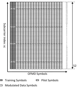
Figure 2.3 DSRC transmission packet format (time vs. frequency domain grid) ... 14

Figure 2.4 Transmitter model of the DSRC system ... 15

Figure 2.5 Convolution Encoder with Rate of 1/2 and a constraint length of K=7 and a generator matrix based on 133 171 8 ... 15

Figure 2.6 Convolution Encoder with Rate of 1/2 and a constraint length of K=3 and a generator matrix of [58 78] ... 16

Figure 2.7 FSM chart for basic convolutional code ... 16

Figure 2.8 Transitions for RSC codes[23] ... 17

Figure 2.9 Transition for NRC codes[23] ... 17

Figure 2.10 Block Interleaver / De-Interleaver ... 18

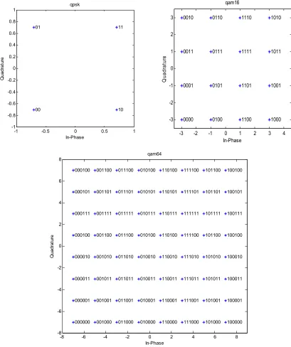
Figure 2.11 Example QPSK (QAM4) Modulated Signal Constellations ... 19

(13)

List of Figures

xii

Figure 2.13 OFDM frame with cyclic extension ... 20

Figure 2.14 DSRC Receiver ... 21

Figure 3.1 Decoding Algorithms ... 24

Figure 3.2 Viterbi Algorithm diagram labels ... 26

Figure 3.3 Viterbi Algorithm for (7, 5) Convolution Encoder ... 28

Figure 3.4 Example of Trellis Diagram for SOVA Decoder ... 30

Figure 3.5 System Diagram of the MAP decoding Algorithm ... 35

Figure 3.6 Gray-Coded of Constellation Points for QPSK, 16 QAM and 64 QAM Mappers ... 36

Figure 3.7 The demapping regions of all message bits sequence ... 38

Figure 3.8 Mapping of 16 QAM In-Phase Symbols into Binary Elements ... 39

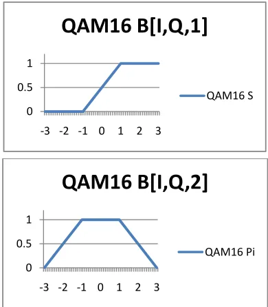
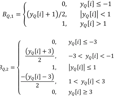
Figure 3.9 S and Π-Decision Rules for 16 QAM ... 41

Figure 3.10 16QAM: Conventional vs. Soft demappers using soft-input Viterbi under Rayleigh fading at 238 km/h ... 43

Figure 3.11 16QAM: Conventional vs. Soft demappers using BCJR under Rayleigh fading at 238 km/h under Rayleigh fading at 238 km/h ... 44

Figure 3.12 16QAM: Conventional vs. soft demappers using both soft-input Viterbi and BCJR under Rayleigh fading at 238 km/h under Rayleigh fading at 238 km/h ... 45

Figure 3.13 16QAM: Conventional vs. Soft demappers using soft-input Viterbi under Ricean fading channel K=1 ... 46

Figure 3.14 QPSK: Conventional vs. Soft demappers using soft-input Viterbi under Ricean fading channel K=1 ... 47

Figure 3.15 QPSK: Conventional vs. Soft demappers using soft-input Viterbi under Rayleigh fading at 238 km/h ... 48

Figure 3.16 16QAM velocity: Conventional vs. Soft demappers using soft-input Viterbi under Rayleigh fading varying velocities at 10dB ... 49

Figure 3.17 QPSK velocity: Conventional vs. Soft demappers using soft-input Viterbi under Rayleigh fading varying velocities at 30dB ... 50

Figure 3.18 16QAM velocity: Conventional vs. Soft demappers using BCJR under Rayleigh fading varying velocities at 30dB ... 51

Figure 3.19 QPSK velocity: Conventional vs. Soft demappers using BCJR under Rayleigh fading varying velocities at 30dB ... 52

Figure 3.20 QPSK: Conventional vs. Soft demappers using soft-input Viterbi under Rayleigh fading at varying high SNR ... 53

Figure 4.1 SISO Decoder ... 54

Figure 4.2 Proposed Receiver Design ... 58

Figure 4.3 Simplified Frequency Domain Channel Model... 59

(14)

List of Figures

Figure 4.5 Proposed vs. Conventional BPSK, QPSK modulation, with and without perfectly known

coefficients at fd=1300Hz ... 67

Figure 4.6 Proposed vs. Conventional BPSK modulation at fd=1300Hz ... 68

Figure 4.7 Proposed vs. Conventional BPSK modulation at fd=550Hz ... 69

Figure 4.8 Proposed vs. Conventional QPSK modulation at fd=1300Hz ... 70

Figure 4.9 Proposed vs. Conventional QPSK modulation at fd=550Hz ... 71

Figure 4.10 Soft Demapping BCJR vs. Proposed... 72

Figure A.1 Illustration of Information exchange between GUI and Simulator ... 81

Figure A.2 Tiered Simulation with each path resulting in dataset for output ... 82

Figure A.3 Modified Tiered Simulation to include Iteration ... 83

Figure A.4 Main GUI page ... 84

Figure A.5 GUI Layout Sections ... 84

Figure A.6 Encoder Settings ... 85

Figure A.7 Decoder Selection process ... 85

Figure A.8 Transmitter and Receiver constants for interoperability between components ... 86

Figure A.9 varying / 0 ... 86

Figure A.10 varying Doppler shift ... 87

Figure A.11 output settings ... 87

Figure A.12 configurable channel properties ... 88

Figure A.13 default action is to create a new simulation message ... 88

Figure A.14 msg load section with new message disabled, showing name of the message to load message. ... 88

Figure A.15 Choose the number of paths ... 89

Figure A.16 choose the channel noise method ... 89

Figure A.17 Different Receivers with different demodulations schemes ... 90

(15)

xiv

List of Abbreviations

The notation used in this thesis is as follows. . and . will be used interchangeably to mean the log-likelihood ratio operation on . . In general, the non-bold face upper case letters denote matrices in time-domain, while bold face upper case letters are used to denote frequency-domain matrices. Non-bold face lower case letters represent the time-domain of one data symbol (modulated symbol), while bold face lower case letters represent the frequency-domain of one data symbol. . denotes a one-dimension array or a signal vector. . represents the modular operation. . denotes the complex conjugate transpose (Hermitian). .* denote a componentwise matrix multiplication, while no operation is used when denoting a regular matrix multiplication, for example A.*B is a componentwise matrix multiplication between A and B. , indicates the row and the column of . Some commonly used

operators, abbreviations and symbols are listed below.

Abbreviation Definition

APP A Posteriori Probabilities

AWGN Additive White Gaussian Noise BCJR Bahl, Coke, Jelinek, Raviv

BCJRA Bahl, Coke, Jelinek, Raviv Algorithm

BER Bit Error Rate

BPSK Binary Phase Shift Keying CIR Channel Impulse Response dB Decibel DFT Discrete Fourier Transform DMC Discrete Memoryless Channel

DSRC Dedicated Short Range Communication FD or fd Doppler Frequency

FEC Forward Error Correction

FER Frame Error Rate

FFT Fast Fourier Transform

(16)

List of Abbreviations

Abbreviation Definition

FSM Finite State Machine

FSSM Finite State Sequential Machine GF(g) Galois or finite field

ICI Inter Carrier Interference

IDFT Inverse Discrete Fourier Transform

IEEE Institute of Electrical and Electronics Engineers IFFT Inverse Fast Fourier Transform

IIR Infinite Impulse Response ISI Inter Symbol Interference

LLR Log Likelihood Rate

MAP Maximum A Posteriori

MAPdec MAP Decoders

MAPEq MAP Equalizer

ML Maximum Likelihood

MMLSE Maximum Likelihood Sequence Estimation

NRC Non-Recursive Codes

OFDM Orthogonal Frequency Division Multiplexing

PDF Probability Distribution Function

PER Packet Error Rate

PHY Physical Layer

QPSK Quadrature Amplitude Modulation RSC Recursive systematic codes

SER Symbol Error Rate

SISO Soft Input Soft Output

SNR Signal-to-Noise Ratio

SOVA Soft-Output Veteribi Algorithm

VA Viterbi Algorithm (Hard-Decision)

WAVE Wireless Access Vehicular Environment

List of Symbols

Coherence Time Coherence Bandwidth

(17)

List of Abbreviations

xvi

Code Rate

OFDM symbol duration Velocity

Carrier Frequency Doppler frequency

. Octal representation

number of constellation points in a modulation scheme modulation waveform at subcarrier

data symbol at subcarrier data rate

time resolution

(18)

Chapter 1 Introduction

In 1999, the U.S Federal Communication Commission (FCC) allocated a 75 MHz spectrum at 5.9 GHz for Dedicated Short-Range Communication (DSRC) system for services that involve vehicle-to-vehicle and vehicle-to-roadside communications [1]. Although the DSRC band is a licensed spectrum, the FCC does not charge a fee for its usage [1]. The main purpose of its establishment is for improving road safety. The program, which is referred to as ‘Vehicular Infrastructure Integration’ (VII), is being considered by the United States Department of Transportation (USoT) [2]. The DSRC system is a short to medium range communication system, i.e. the distance range between the transmitter and the receiver should be around a 1000 meters. That is, unlike some other radio communication systems such as cellular or FM radio, where their communication range are in kilometres and hundreds of kilometres, respectively [3].

DSRC is also known as the IEEE 802.11p Wireless Access in Vehicular Environment (WAVE) [1], [2], and was based on the IEEE 802.11a standard [4]. The main difference between these two standards is the increase of the symbol duration in DSRC that resulted from the 10 MHz reduction in the channel spacing compared to the IEEE 802.11a standard, with 20 MHz channel spacing. IEEE 802.11a is one of the standards used in wireless local area network (WLAN), and was designed for time-invariant channels suitable for stationary indoor environments with low delay spread; hence it makes sense to extend the symbol duration in DSRC, which was justified in [5]. The DSRC physical layer, which is the main focus of this thesis, employs orthogonal frequency division multiplexing (OFDM) physical layer technique [6]. OFDM is popular for its ability to mitigate inter symbol interference (ISI) through the use of sufficient guard interval.

(19)

1. Introduction

2

1.1 Orthogonal Frequency Division Multiplexing

The basis for the DSRC Physical Layer is that of the 802.11a OFDM transmitter/receiver combination. Orthogonal Frequency Division Multiplexing (OFDM) uses a single serial transmission that contains multiple subcarriers. OFDM was first introduced by Chang and Gibby in [6], for the purpose of transmitting information across harsh channel environments. This technique works by joining equally spaced subcarriers into one serial transmission using IFFT transformation.

The IFFT/FFT (Inverse Fourier Transform/ Fast Fourier Transform) are not the only method for modulation/demodulation in OFDM. Actually, in [7] the IFFT/FFT methods were shown to produce similar results to a different method used to generate the OFDM system and its orthogonality. The modulation uses oscillators and the demodulation uses matched filters (correlator implementation) as shown in Figure 1.1(a) and (b), respectively.

0

1 0

1

(a)Transmitter

0

1

0

1

(b) Receiver

Figure 1.1 (a) Multi-carrier Modulation and (b) Demodulation Using Correlators

The OFDM signal can be written as follows [8],

(20)

1. Introduction

where:

is the modulated multi-carrier signal and at time t.

is the data symbol at subcarrier, where 0, 1, 2, … . , . is the modulation waveform at subcarrier and at time .

This relationship is also shown in Figure 1.1(a). For orthogonality the modulation waveform is chosen as a set of orthogonal waveforms [9][8],

1

, 0, 0,

(1-2) is the frequency of the subcarrier. We can note that the window restriction of 0, gives us the sinc functions that we see in frequency domain, as shown in Figure 1.2. The different colorings and/or symbols on the sinc function plots represent different subcarriers that are orthogonal to one another (sc1, sc2, sc3, sc4).

For the demodulation equation of Figure 1.1(b), we get [8],

(1-3) where

is the modulated multi-carrier signal and at time t.

is the demodulated data symbol of subcarrier, where 0, 1, 2, … . , . is the complex conjugate of .

Figure 1.2 Spectrum of the OFDM signal with 4 subcarriers

(21)

1. Introduction

4 using the Inverse Discrete Fourier Transform (IDFT) or the Inverse Fast Fourier Transform (IFFT) to get

the symbol ready for transmission in the time domain, and conversely in the receiver, the DFT or FFT algorithms are used during the demapping, as shown in Figure 1.3.

-Point IFFT

Insert

Guard

-Point FFT

Remove

Guard

Cha

n

el

(a) Transmitter

(b) Receiver

Figure 1.3 OFDM (a) Transmitter and (b) Receiver Systems

A cyclic prefix guard interval can be inserted before transmission and removed after reception (as seen in Figure 1.3) to reduce Inter Symbol Interference (ISI), which becomes the main benefit for OFDM systems when combating harsh channel environments. This is because the low symbol rate makes the use of a guard interval between symbols affordable, giving rise to the possibility of handling time spreading and eliminating ISI. The guard interval will be described in more details in Chapter 2 when the DSRC system model is defined.

OFDM has high spectral efficiency which permits high throughput data transmission in a small frequency band. As already expressed, the orthogonality of the subcarriers allows for overlapping subcarriers to still be separated, i.e. no interference at the carrier locations. Figure 1.2 illustrates how the subcarriers are overlapping. Although the guard interval helps combat ISI, increasing it reduces the spectral efficiently because of the extra redundancy.

(22)

1. Introduction

Additionally, 802.11a/g/n, HYPERLAN/2, Digital audio and video broadcasting, i.e. DAB and DVB, WLAN, 802.20 Mobile Broadband Wireless Access and 802.16e WiMax standards all use OFDM as physical transmission modes.

1.2 WAVE Channel Model

Multipath fading and Doppler shift are two physical phenomena that are encountered in wireless communication systems between two Omni-directional antennas with nonzero relative velocity. Multipath refers to both line-of-sight (LOS) and non-line-of-sight (non-LOS) components, due to the reflections of the transmitted signals by the surrounding objects. Multipath may cause what is known as “frequency selective” fading, which induce inter symbol interference (ISI) when the symbol duration or symbol period ( ) is less than 10 times the multipath RMS delay spread (σ_τ , ( 10σ_τ . The channel may be considered flat if the range of the channel frequencies or coherence bandwidth ( satisfies [10],

1

50σ_τ (1-4)

In time-varying channels, a nonzero relative velocity is produced, because both antennas may be moving towards each other or in the same direction but at different speeds. The resulting maximum Doppler shift ( ) is related to the relative velocity via the equation . ⁄ , where is the relative velocity in meters per second ⁄ , is the carrier frequency in Hertz (Hz), and is the speed of light in ⁄

[10]. Also, the channel may be characterized as a “fast fading” channel if . , where is the coherence time and is the number of OFDM symbols per packet,

0.423 0.423 . ⁄

0.423 .

. µ _(1-5)

In other words, the channel impulse response is changing within the duration of a symbol or packet if or . is not satisfied, respectively. Since and remain constant throughout a particular system, the rate of fading is proportional to one of the parameters , while the others remain constant. Rician fading channel could be used if a strong LOS component exists, while Rayleigh fading could be considered when time-varying channels exist with No-LOS.

(23)

1. Introduction

6

offset oscillators

Figure 1.4 Jakes Fading Simulator

Jake’s method works by simulating the physical model of 2D isotropic scattering with no-LOS. It assumes that there are N equi-spaced or uniformly distributed scatters around the vehicle,

2

, 1,2, … , _(1-6)

The phase angle associated with each scatter is chosen at random. The received complex envelope is treated as wide-sense stationary Gaussian random process with zero mean, when Rayleigh channel is concerned. The WAVE (wireless access vehicular environment) channel model can be modeled using statistical methods presented in [12] [13].

Figure 1.5 illustrates the WAVE channel model. It has both specular and scatter components. It is a model for simulating the effects of an L number of paths Rayleigh/Rician multipath scattering channel with AWGN and K factor affecting specular to scatter component fading path ratio.

1 2

1

2

1 1

1

Specular Component

S(t) _ComponentScatter

r(t)

(24)

1. Introduction

Referring back to Figure 1.4, and in order to produce a zero mean Gaussian envelope, the following relation is used [12][13],

(1-7)

√2 2 2 √2 2

2 2 √2 2

(1-8) where β . We need M number of oscillators with frequencies,

2

, 1,2, … , _(1-9)

According to [15] greater than 6 should suffice.

a) 27 Hz

b) 550 Hz

c) 1300 Hz d) 3800 Hz

(25)

1. Introduction

8

a) 27 Hz

b) 550 Hz

c) 1300 Hz _{d) 3800}_Hz

Figure 1.7 view of scatter plots showing QPSK constellation distortion under various frequency shifts (vertical represents data samples)

(26)

1. Introduction

Figure 1.9 dispersion of amplitude and phase in the time domain for QPSK with no AWGN

Figure 1.10 side view of dispersion of amplitude and phase in the time domain for QPSK with no AWGN

In order to visually demonstrate the effect of the channel on the message bits, scatter plots in Figure 1.6 are produced for 5.9 GHz DSRC system over a 1 packet of duration of 0.64 , using QPSK modulation scheme. Different Rayleigh fading envelopes are simulated using different velocities. Additive white Gaussian noise (AWGN) is also considered using different signal-to-noise ratio (SNR) values. As illustrated from the figure, as the velocity is increased there exist a greater shift in both amplitude and phase, which result in the deviation of the received symbols from their constellation points. As for AWGN, the increased velocity produces a more scattered version of the symbols, hence increases the chance of erroneously interpreting symbols. Figure 1.7 represent the 3-D version of Figure 1.6.

(27)

1. Introduction

10

a) b)

c) d)

0 500 1000 1500 2000 2500 3000 3500 4000 0 0.2 0.4 0.6 0.8 1 1.2 1.4 1.6 1.8 2

samples (time*80τ)

m

agni

tude

80 OFDM symbols, 1 packet, with Doppler Frequency =27Hz

0 500 1000 1500 2000 2500 3000 3500 4000 0 0.2 0.4 0.6 0.8 1 1.2 1.4 1.6 1.8 2

samples (time*80τ)

m

agni

tude

0 500 1000 1500 2000 2500 3000 3500 4000 0 0.2 0.4 0.6 0.8 1 1.2 1.4 1.6 1.8 2

samples (time*80τ)

m

agn

itud

e

0 500 1000 1500 2000 2500 3000 3500 4000 0 0.2 0.4 0.6 0.8 1 1.2 1.4 1.6 1.8 2

samples (time*80τ)

m

agn

itud

e

Figure 1.11 Samples vs. magnitude of 1 packet, 80 OFDM symbols under varying doppler frequencies

Figure 1.11 above, provide us with the information about the effect that the doppler frequencies have upon the data symbols. It can be seen here, that as the doppler frequencies increase the transmitted data experience the so-called deep fades, which represent the amplitude attenuation on the particular samples at the time that these deep fades occur.

1.3 Organization of the thesis

Previous sections provided a description of the OFDM system and the channel model, which are two critical components or factors that are needed to be understood in order to ensure successful state of the art design. What follows is the organization of this thesis:

Chapter 2 contains the description of the conventional DSRC system (or 802.11p) similar to that of the 802.11a standard [4], [16].

(28)

1. Introduction

Chapter 4 presents the detailed description of the proposed receiver design for enhancing the performance of the DSRC system using frequency domain MAP equalization algorithm.

Chapter 5 summarizes major accomplishments and suggestions for future research studies are given in this chapter.

(29)

12

Chapter 2 FEC coded and OFDM DSRC systems

2.1 Channel Coding Theory

Claude Shannon [17], "the father of information theory" [18], introduced the main concepts of information theory. Shannon went beyond the examinations of signals' frequencies, bandwidths and noise added to them during transmission [19]. He characterized the source that produces these messages and proved that there exists a theoretical limit at which error-free communication could take place using error-correcting codes. Several coding schemes in hopes of achieving this Shannon limit performance were developed. This family of codes are called Forward Error Correcting (FEC) codes. They are mainly composed of two parts: the convolutional and the block codes. FEC code went from a single error correcting code technique called Hamming block code, to maximum likelihood sequence algorithm Viterbi [20] for decoding convolutional code. Due to the famous Viterbi algorithm, convolution coding was more exploited and hence became more popular. The Viterbi decoder will be discussed in Chapter 3 along with maximum a-posteriori (MAP) and maximum likelihood (ML) decoders, which will be used in our DSRC receiver design. The description of the conventional DSRC system is presented in this chapter.

2.2 The DSRC System Model

Insert Pilots

64 80

64 Binary

Input

To Channel Convolution

Encoder π Mapper S/P IFFT

Add

CP P/S

a) Transmitter

Signal

Compensator 64 64

64

S/P Remove

CP P/S Demapper π'

Viterbi

Decoder

48

FFT Binary

Output

Channel

Estimator

From

Channel

Remove

Pilots

80

b) Receiver

(30)

2. FEC coded and OFDM DSRC systems

In this section we describe the DSRC system model in both the time and the frequency domain baseband model. Figure 2.1 shows the block diagram of the DSRC system model. DSRC physical layer (PHY) uses OFDM to mitigate the effect of ISI by using guard interval that exceeds the maximum excessive delay. The guard interval is added at the transmitter and later removed at the receiver. It is a copy of the symbol tail and placed in front of the symbol, known as a cyclic prefix. Its duration is usually computed as around 20% of the OFDM symbol duration. DSRC is very similar to the 802.11a standard [4] with the difference being in doubling the symbol duration in the case of the DSRC system. In DSRC, the guard interval is 1.6 with symbol duration of 8.0 and signal bandwidth of 10MHz. Figure 2.2 shows the packet format of the DSRC system.

GI2 GI SIGNAL GI GI … GI

8

8 1.6 + 6.4 = 8

16 + 16 = 32

10 + 1.6 = 16 16

Figure 2.2 DSRC transmission sequence

It consists of a short and a long preamble. The short preamble is used for frequency offset estimation and symbol timing, while the long preamble is used for channel estimation through the use of two identical training symbols [4] . The guard intervals can also be seen in Figure 2.2. The DSRC symbol length is composed of the OFDM symbol length {64} and the guard interval length {16}. The minimum time resolution 0.1 is (resulting in 10MHz channel spacing). The number of subcarriers is 48 , and the symbol period is 8 ), the data rate of a DSRC system depends on both the modulation scheme and the code rate as follows,

. . N

(2-1) The term gives the number of bits per modulated data symbol.

From Figure 2.1, the binary message goes through a series of components before transmission. First it goes through a convolution encoder with a generator of (133 , 177 ) and constraint length of 7 for forward error correction coding (FEC) reasons. The encoded message is then interleaved to avoid long burst errors due to fading and AWGN. The interleaved message is then digitally modulated using one of the Gray-Coded constellations BPSK, QPSK, 16 QAM, and 64 QAM [4] . The resulting modulated message is then divided into 64 shorter and parallel data symbols , (includes 4 pilot symbols, and 12 zero-padding), for the

OFDM symbol in size packet (0, 1, …, 1), and the sample point (subcarrier: 0, 1, …, ( 1 63)) of the OFDM symbol. The pilot symbols are inserted in the 6th_{, 20}th_{, 34}th_{, and 48}th

(31)

14

1; 16) after the addition of the guard interval, and then serially transmitted over the channel. In order to satisfy equation (1-4) and with high delay spread involved in vehicular environments, the spacing of these pilots’ tones needs to be at least 200KHz[21]. Hence, with the pilot spacing set as 1.85 MHz for the DSRC system, channel estimation using the current pilots is not feasible.

2.3 The DSRC Transmitter

As mentioned earlier, the DSRC 802.11p (WAVE) is an amendment to the IEEE 802.11a standard. Some of the revisions will be highlighted here. After the description of the DSRC transmission packet format, the blocks that make up the transmitter will be described.

` +26 +24 +25 +23 +22 +21 +20 +19 +18 +17 +16 +15 +14 +13 +12 +11 +10 +9 +8 +7 +6 +5 +4 +3 +2 +1 ‐1 ‐2 ‐3 ‐4 ‐5 ‐6 ‐7 ‐8 ‐9 ‐10 ‐11 ‐12 ‐13 ‐14 ‐15 ‐16 ‐17 ‐18 ‐19 ‐20 ‐21 ‐22 ‐23 ‐24 ‐25 ‐26

OFMD Symbols

Su bc arrie r inde x: sc

Training Symbols

Modulated Data Symbols

Pilot Symbols

52

Figure 2.3 DSRC transmission packet format (time vs. frequency domain grid)

(32)

2.3.1 Convolution Encoder

Figure 2.1(a) shows the transmitter model of the DSRC system. For convenience, it is also shown below.

Insert Pilots

64 80

64 Binary

Input

To Channel Convolution

Encoder π Mapper S/P IFFT

Add

CP P/S

Figure 2.4 Transmitter model of the DSRC system

Convolution Encoding is frequently used for Forward Error Correcting (FEC) coding in communication systems. A convolution encoder can be described as a markov finite state machine which takes input as information bits and provides outputs as coded bits. In other words, the convolution encoder takes in statistically independent values from a discrete alphabet and outputs a sequence of values that are also taken from a statistically independent discrete alphabet [22]. The convolutional encoder can be represented by a generator sequence which is a set of impulse responses, whereby each information bit must pass through the generator constraint Length number of steps before the encoding is complete.

, , … ,

(2-2) where is the constraint length, and is from 1 to the number of outputs.

The number of inputs over the number of outputs of a convolutional code defines the code rate

/ (i.e. for a 1 input, 2 output convolutional code, the code rate is said to be 1/2).

The encoding process is dependent on a trellis structure that defines the rate, and input/output relationship. A rate 1/ convolutional encoder can be represented as a finite state machine (FSM) with the state of the encoder defined by the contents of 1 shift registers. The 802.11 Standard [4] defines the OFDM PHYS for which DSRC is based, and uses the industry standard 133 ; 171 generator matrix as seen in Figure 2.5.

Z1 Z2 Z3 Z4 Z5 Z6

input

Output Data 0

Output Data 1

1338

(1011011)

2 ₁₇₁

8

(1111001)

(33)

16

The FSM describing information forms a trellis that shows the paths that the encoding take from one state to the other over time.

The output of the convolution encoder can be obtained by performing the discrete convolution,

(2-3) where * denotes the modulus-2 convolution.

Figure 2.7 shows an example of a FSM of a basic convolutional encoder example shown in

Figure 2.6 , i.e. a convolution encoder with Rate of 1/2 and a constraint length of K=3 and a generator matrix of [5 7 ], and Table 2-1 shows its state transition.

Z1 Z2

input

Output Data 0

Output Data 1

5₈ (101)

2 ₇

8

(111)

Figure 2.6 Convolution Encoder with Rate of 1/2 and a constraint length of K=3 and a generator matrix of [5 7 ]

0

2

1

3

Figure 2.7 FSM chart for basic convolutional code

(34)

Table 2-1: State transition of convolution example

In Current

State

S Next

State

S O1 O2

0 0 0

0 0 0 0 0 0

1 0 0 1 0 2 1 1 0 0 1

1 0 0 0 1 1

1 0 1 1 0 2 0 0 0 1 0

2 0 1 1 1 0

1 1 0 1 1 3 0 1 0 1 1

3 0 1 1 0 1

1 1 1 1 1 3 1 0

State 0

State 1

State 2

State 3

1‐Transition

Branches

0‐Transition

Branches

time t‐1 time t

Figure 2.8 Transitions for RSC codes[23]

State 0

State 1

State 2

State 3

1‐Transition

States

0‐Transition

States

time t‐1 time t

Figure 2.9 Transition for NRC codes[23]

(35)

18

meaning a portion of recursive decoder output depends directly on the input. While, the non-recursive codes do not.

Decoding of the convolutional code can be done by Viterbi algorithm [20] for Maximum Likelihood, or the BCJR for Maximum a posteriori [24] and are discussed in details in the next chapter.

2.3.2 Interleaving

Because of the fact that fading channels may have deep fades that can cause a long sequence of errors, a method used in combating burst errors is interleaving. Interleaving has the effect of reducing adjacent correlation in the bit stream. This can be done either pre-symbol mapping known as bit interleaving or post-symbol mapping, which is symbol interleaving.

Write‐>

Re

ad

‐

>

Read‐>

Message:

Interleaver: De‐Interleaver:

Message:

Message: 1 2 3 4

5 6 7 8

9 10 11 12 13 14 15 16

1 2 3 4

5 6 7 8

9 10 11 12 13 14 15 16

<

‐

Wr

ite

5 6 7 8

1 2 3 4

9 10 11 12 13 14 15 16

1 2 3 4 5 6 7 8 9 10 11 12 13 14 15 16

1 ₂

3 ₄

9 ₁₀

11 ₁₂

13 ₁₄

15 ₁₆

5 ₆

7 ₈

Figure 2.10 Block Interleaver / De-Interleaver

Both the interleaving and de-interleaving process can be done with different size blocks. Figure 2.10 shows the interleaver for a 4 row, 4 column block interleaver and de-interleaver showing the dispersed correlation of the interleaved ( ) message from adjacent bits. In the interleaving example, each data symbol (numbered 1 though 16 in this case) is written to the rows of the interleaver block of size r=4, c=4. The interleaving is actually just a rotated read, which reads each data symbol column wise and concatenates the result to achieve the message. The deinterleaving process is the reverse in that columns are written to first and then the reading is done row wise. Giving the final result in the receiver of data that was in the original order as it originally was in the transmitter.

(36)

2.3.3 Modulation

-1 -0.5 0 0.5 1

-1 -0.8 -0.6 -0.4 -0.2 0 0.2 0.4 0.6 0.8 1 Quadr at u re In-Phase QPSK Modulation Constellation Points

Figure 2.11 Example QPSK (QAM4) Modulated Signal Constellations

-1 -0.5 0 0.5 1

-1 -0.8 -0.6 -0.4 -0.2 0 0.2 0.4 0.6 0.8 1 Q uad rat ure In-Phase bpsk

-1 -0.5 0 0.5 1

-1 -0.8 -0.6 -0.4 -0.2 0 0.2 0.4 0.6 0.8 1 Q uad rat ure In-Phase qpsk

-1 -0.5 0 0.5 1

-1 -0.8 -0.6 -0.4 -0.2 0 0.2 0.4 0.6 0.8 1 Q uad rat ure In-Phase qam16

-1 -0.5 0 0.5 1

-1 -0.8 -0.6 -0.4 -0.2 0 0.2 0.4 0.6 0.8 1 Q uad rat ure In-Phase qam64

Figure 2.12 Normalized signal constellations

(37)

20

As mentioned earlier, the modulations chosen can be BPSK, QPSK, QAM16, or QAM64, with modulation levels of log 2, log 4, log 16, and log 64, respectively.

After modulation, the complex data symbols should be grouped into 48 complex numbers for being used in the IFFT. The complex numbers will be numbered from 0 to 47 and mapped onto spaced data coordinated

with 4 pilot symbols in between as shown in Figure 2.3.

Figure 2.12, below shows the normalized signal constellations for BPSK, QPSK, 16 QAM and 64 QAM.

2.3.4 IFFT

The Inverse Fast Fourier Transform is used to transform the modulated signal to the time domain for transmission as a serial transmission.

, , (2-4)

Where, . is the Inverse Fast Fourrier Transform (IFFT). x , and , are the time domain output

and the frequency domain input to the IFFT block at the OFDM symbol, and the subcarrier, respectively.

2.3.5 Guard Interval

The guard interval is a redundant portion of the transmission, a cyclic extension of the tail bits added to the beginning of the message to absorb inter-symbol interference in the time domain.

Figure 2.13 OFDM frame with cyclic extension

(38)

be 125000 for DSRC, making 8 , hence 80 640 . For our analysis we are

ignoring the overlap length shown in Figure 2.13, because we are not addressing synchronization in this thesis.

2.4 DSRC Receiver

This section will present a description of the DSRC receiver of Figure 2.14.

Signal

Compensator

64 64

64

S/P Remove

CP P/S Demapper π'

Viterbi

Decoder

48

FFT Binary

Output

Channel

Estimator

From

Channel

Remove

Pilots

80

Figure 2.14 DSRC Receiver

The DSRC Receiver must cope with potential fading due to the high velocities and multipath fading in urban environments. The goal of reconstructing and obtaining the original transmission message can be challenging (if not impossible) if too much of the signal has been distorted or lost.

The receiver receives the signal and will attempt to correct errors that may have occurred during transmission through a Rayleigh faded and AWGN channel. The components that assist with error correction and/or prevention are the Guard Interval, Channel Estimator and Signal Compensator, FFT, Interleaver, and Decoder.

2.4.1 The time domain

At the receiver, the reverse of the transmission process starts to unfold. The received signal vector of one OFDM symbol is,

(2-5)

Where is the channel impulse response (CIR) vector and can be expressed as

_, _, . . _{, 0} ₁

(2-6) where N is for number of OFDM subcarriers, , is the complex impulse response for the path of the

(39)

22

, . , 0 1

(2-7)

2.4.2 The frequency domain

After the removal of the guard intervals from the received data (or channelword), the parallel data symbols , can be expressed in terms of a matrix

. . (2-8)

The variables , and are 1 vectors (N is for number of OFDM subcarriers). is the discrete Fourier transform (DFT) of size ( is the number of OFDM symbols in a packet). . denotes the complex conjugate transpose (Hermitian). is the time-domain channel matrix (circulant if the channel is time-invariant).

After that, the signal is demultiplexed and fast Fourier transformed (FFT) into the frequency domain output as follows,

, , . , , _(2-9)

where , , , , , , , denote the FFT of the received OFDM symbols, the channel response, the

transmitted OFDM symbols, and the AWGN of the OFDM symbol at the subcarrier, respectively.

2.4.3 Channel Estimation

The first two OFDM symbols called the training symbols, as shown in Figure 2.3, are then used in the channel estimation process. The channel estimation block estimates channel distortion and relays that information to the signal compensator to attempt to reconstruct the signal back to its undistorted form. Assuming that , is known, then the channel frequency response can be obtained as follows,

, , ,

,

, ,

,

, , , (2-10)

Using two training symbols instead of 1 minimizes the effect of , reducing noise enhancement by the signal compensator. Therefore, the two training symbols are used in obtaining the estimated channel response over the first two received symbols as follows,

, _2., ,

, , , ,

(40)

2.4.4 Signal Compensation

As shown in Figure 2.14, 1-tap signal compensator is used in the 802.11a standard to estimate the transmission distortion based on the channel estimation derived by the channel estimator using two training symbols. At the output of the signal compensator, the received OFDM symbols are compensated as follows,

, ,

,

(2-12) The compensated symbols are then digitally demodulated, deinterleaved and finally decoded using a Viterbi decoder [20] , [4].

2.4.5 Demodulation and Deinterleaving

Demodulation, deinterleaving as inverse of their transmitter counter parts. Special care must be taken for soft demodulation if using a soft input decoder for preserving probability information. Soft demodulation is covered in the next chapter.

2.4.6 Decoding

Maximum likelihood (ML), Viterbi decoder [20] , [4] is used to decode the convolutional codes. Next chapter will have a detailed description of the Viterbi algorithm.

(41)

24

Chapter 3 Hard vs. Soft Decoding Algorithms and Proposed Soft Demapping

Scheme

Chapter 3 Hard vs. Soft Decoding Algorithms and Proposed Soft

Demapping Scheme

In the previous chapter, the DSRC system was introduced. This chapter will be dedicated for deriving the algorithms behind the Viterbi decoder used in the conventional DSRC system and the BCJR algorithm in order to use them along side with our proposed demapping scheme that is introduced in this chapter. Figure 3.1 below shows the overall trellis-based algorithms used in decoding. Our proposed system in Chapter 4 will be developed using the trellis-based MAP BCJR algorithms [24].

Figure 3.1 Decoding Algorithms

Information about the improved SOVA can be found in [25]. This chapter will present three different demapping schemes and compared with one another using both Viterbi [20] and BCJR [24] decoding schemes, under varying signal to noise ratio (SNR) and velocities. They will also be compared under different environments, i.e. Rayleigh and Rician faded channels. The next chapter (4)will present a receiver design for DSRC system that utilizes the concept behind the MAP algorithm (BCJR), which greatly outperforms the conventional system in both bit-error-rate (BER) and packet-error-rate (PER).

Trellis-Based Algorithms

Viterbi MAP/BCJR

SOVA

Improved SOVA

Log-MAP

(42)

3. Hard vs. Soft Decoding Algorithms and Proposed Soft Demapping Scheme

3.1 Optimal detection in the estimation of the states of a Markov process

The goal of an optimal receiver is to reproduce the message ( that was sent at the transmitter as accurately as possible. In other words, the receiver most be able to minimize the probability of error

for each message bit . The way to achieve that is to maximize the a posteriori probability (APP) | [26], where is the observed sequence array. Therefore, for optimal detection, we have:

|

(3-1) Where the symbol ‘ ’ is used to indicate that the value or bit is an estimated one, that is, a value or bit after it undergoes some sort of a process in the receiver of a system, like demapping, deinterleaving and decoding. The equation above turns out to be the main inspiration of the symbol by symbol (MAP) or Maximum a posteriori BCJR algorithm [24]. The Map algorithm tries to find the most likely transmitted symbol , given the received sequence . The BCJR algorithm will be explained in more details in the next few sections.

The Viterbi [20] algorithm is another well known algorithm that is used to estimate the states of a Markov process, but the difference between it and the BCJR algorithm is in the fact that the Viterbi algorithm tries to find the most probable transmitted sequence ( given the received sequence , instead of what was mentioned about the BCJR algorithm in the previous paragraph. Therefore, it follows for the Viterbi algorithm that:

|

(3-2) From this brief introduction, it can be seen that the BCJRA (BCJR algorithm) minimizes the symbol error rate (SER), while VA (Viterbi algorithm) minimizes the frame error rate (FER).

3.2 The Viterbi Algorithm (VA/SOVA)

(43)

26

3.2.1 Harddecision Viterbi (VA)

Hard-decision Viterbi [20] receives hard channel-bits that were given by the demodulator/demapper. Demodulator and demapper will be used interchangeably throughout this thesis. The demapper makes a decision on the channel-bits that it receives from the signal compensator and maps them into binary values (‘0’ or ‘1’) according to the constellation points that is used in a modulator scheme at the transmitter. These binary values are then fed to the Viterbi decoder as input and the Viterbi decoder produces its own decoded hard decision of the message.

The Viterbi algorithm (VA) is best understood with an example. If we use the NRC encoder introduced in Chapter 2 as our example, we will see that the encoder encoded data-words, by constructing specific paths through a trellis diagram. Having the trellis as a tool, the Viterbi decoder knows that there exist specific transitions from one state to another. For example and for simplicity, let us assume a data-word (original message) of [0 0 0 0]. This message is first encoded to become the code-word of [00 00 00 00]. This codeword is then corrupted when sent through a noisy channel to become the channel-word [10 00 10 00]. Now, we will attempt to decode this channel-word. Figure 3.3 below shows the process of decoding the received channel-word by determining the most likely path using the trellis information generated by the convolution encoder of Figure 2.6.

Figure 3.2 defines the important terms used in defining the VA. The branch metric or Hamming distance in our case is the number of bits which differ between two binary strings. The branch labels are the code-words corresponding to the path of one state to the next defined by the convolution encoder’s trellis. For example, the branch label or code-bits from ‘state 0’ to ‘state 0’ is always ‘00’ for the convolution encoder of Figure 2.6

.

Figure 3.2 Viterbi Algorithm diagram labels

1

1 S=0

00;11

S=1

11;00

S=2

10;01

S=3

01;10

States/Possible outputs

0 transition

1 transition

Hamming Distance

=Branch Metric

00

(44)

1

2

3

2 S=0

00;11

1 0

0 0

Channel-Words

S=1

11;00

S=2

10;01

S=3

01;10

00

11

10

01 (a)

1

2

3

2

3

4

2

3

5

2 S=0

00;11

1 0

0 0

1 0

Channel-Word

S=1

11;00

S=2

10;01

S=3

01;10

00

11

(45)

28

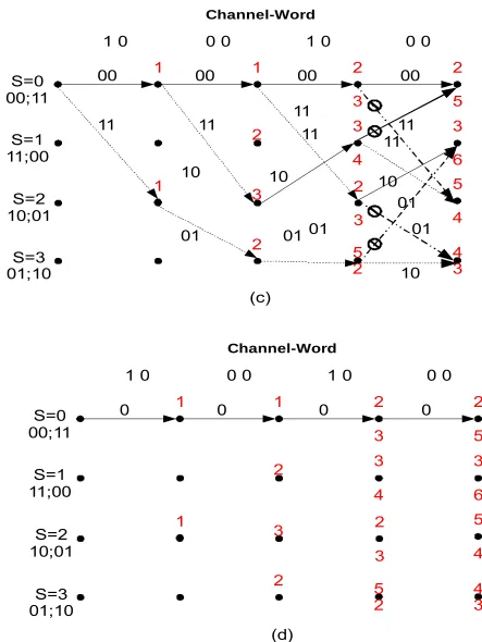
Figure 3.3 Viterbi Algorithm for (7, 5) Convolution Encoder

1

2

3

2

3

4

2

3

5

2

5

3

6

5

4

3 S=0

00;11

1 0

0 0

1 0

0 0

Channel-Word

S=1

11;00

S=2

10;01

S=3

01;10

00

11

10

01

10

01

11 ₁₁

10

01

10

01 (c)

1

2

3

2

3

4

2

3

5

2

5

3

6

5

4

3 S=0

00;11

1 0

0 0

1 0

0 0

Channel-Word

S=1

11;00

S=2

10;01

S=3

01;10

0

(46)

The encoder is composed of two memory blocks that is there are four possible states. Since the encoder is assumed to have started from state zero, then the VA starts at the initial state zero. As shown in Figure 3.3, the code-bits from state ‘0’ to state ‘0’ is expected to be ‘00’, and ‘11’ for the state ‘0’ to state ‘2’. The channel-bits at t=1 are corrupted and were received as ‘10’. At that time, that is at that beginning state ‘0’, the encoder have either gone from state ‘0’ to state ‘0’ (itself) or to state ‘2’. This means that there are two possible paths that the trellis would have taken. The branch metrics or Hamming distances between these initial received channel-bits (10) and the possible code-bits (00 and 11) for both paths (S=0 to S=0 and S=0 to S=2) respectively would be ‘1’ for both paths. Next, the channel-bits at time t=2 will be considered, that is 00. At time t=2, we now have to “active” states that will be considered in the trellis to arrive their next states. In other words, the present states at this time are S=0 and S=2. Again for S=0, the only possible next states are S=0 and S=2 and as for S=2, the only possible next states are S=1 and S=3, each with their own branch labels or possible code-bits (10 and 01 respectively). The received channel-bits here are 00, which correspond to Hamming distances of (0, 2, 1, 1) for (S=0 to S=0, S=0 to S=2, S=2 to S=1, S=2 to S=3) respectively. Note that these Hamming distances were just for that time slot t=2. Therefore, before going to time t=3, we add all the Hamming distances obtained in the prior time slot or states with paths connecting to the next states, specifically (1, 3, 2, 2) for (S=0 to S=0, S=0 to S=2, S=2 to S=1, S=2 to S=3) respectively as seen in Figure 3.3(a). S=1 and S=3 are now been added to the equation. S=1 can only go to the next states S=0 (with only possible bits of 11) and S=2 (with only possible bits of 10), while S=3 can only go to the next states S=1 (with only possible bits of 01) and S=3 (with only possible bits of 10). Using the same procedure, we obtain the total Hamming distances for t=3 Figure 3.3(b). Before proceeding to time t=4 in Figure 3.3(c), we see that the paths start to merge together (Figure 3.3(b)), which cause “conflict”, hence a decision has to been as to which paths need to “stay” and which paths need to be “eliminated”. The paths marked with the symbol “ ” are the eliminated paths. Elimination occurs on the paths with the higher accumulated metric at the “conflict” points. In Figure 3.3(b), we can see the paths from (S=1 to S=0, S=1 to S=2, S=2 to S=3, S=3 to S=1) are eliminated as they have higher accumulated metric values against (S=0 to S=0, S=0 to S=2, S=3 to S=3, S=2 to S=1) respectively. This process is continued until the end of the received channel-bits, where the path with the lowest accumulated metric is chosen as seen in Figure 3.3(d). That “winner” or “survivor” path is called the survivor path. Therefore, the final decoded message is [0 0 0 0], due to the fact that these bits correspond to the inputs that follow these survivor path created by the trellis encoder.

(47)

30

always 4 survivor paths for t 2. Therefore, for convolution encoder, we will have 2 survivor paths after t n 1 for constraint length ‘n’ (Recall 1). It can therefore be concluded that the Viterbi algorithm is not an ideal decoding scheme when a large constraint length is used, due the exponential increase of the number of survivor paths with increasing constraint length.

3.2.2 Softdecision Viterbi (SOVA)

Although the demappers of this chapter will not include Soft-input soft-output Viterbi algorithm (SOVA), but it is worth defining it here as it is an important decoding scheme when it comes to turbo decoding. In other words, when the VA is to be used in turbo decoding, then SOVA replaces the soft-input VA. As it will be seen in the next chapter, it is necessary to have the decoders be able to accept soft information as their inputs and produce soft output information when it comes to turbo decoding. However, SOVA is found to be in impractical in some scenarios where minimal delay is required, due to the fact that SOVA is found to work best when large packet length are present, hence creating more delays. This section will present the Viterbi algorithm with soft-input and soft-output capabilities.

+1 +1 +1 +1

-1 -1 -1 -1 +1 -1

+1 -1

-1 +1

-1.8 -0.2

-0.4 1.4 1.6

0 0

-1.6

-1.6 4.6 S=0

S=1

S=2

S=3

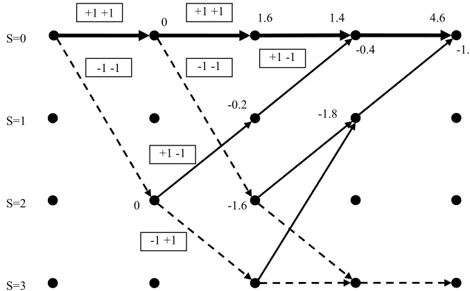
Figure 3.4 Example of Trellis Diagram for SOVA Decoder

Table 3-1: Example of SOVA Decoder

Modulated

Message:

+1 +1 +1 +1

Codeword:

+1+1

Channelword:

+0.9 -0.9

+0.7 +0.9

+0.9 +1.1

+1.7 +1.5

Decoded

Modulated

Message :

(48)

SOVA was proposed by [27] in 1989, which is similar to VA, but with slight modification. SOVA outputs a posteriori probabilities (APP). The main difference is in how the branch metric is calculated. An example of how these branch metrics are calculated is given in Figure 3.4 and Table 3-1. To obtain the APP, the SOVA decoder compares the received channelword with the modulated bits instead of the message bit as in the case of VA. For example, in the case of the channelword being +0.9 and -0.9 as in Table 3-1, and assuming that the first state of the Viterbi encoder started at 0 state, this channelword will be have two possible next states (0 and 2) and could only have produced the channel bits +1 +1 or -1 -1. Therefore, the channelword will be multiplied by these possible channel bits and added together as follows: for the case of channel bits +1 +1 Î (+0.9)(+1) + (-0.9)(+1) = 0, while for the channel bits -1 -1 Î (0.9)(-1) + (-0.9)(-(0.9)(-1) = 0. There we would see the branch metric as 0s for both transitions. The calculations will carry on in this manner until it reaches the final stage where all the channelwords were taken into account. The final decision is made, such that the path with the highest or largest accumulated probability value or branch metric value will be chosen to be the correct path.

3.3 BCJR/ MAP (Maximum A Posteriori) Algorithm

Decision rules can be classified as either maximum likelihood rule, where the databit corresponding to the received channelbit is the element with the highest likelihood. The BCJR algorithm (BCJRA) follows a rule that determines the a-posteriori probability 1| or 1| , instead of determining the largest a-priori likelihood function, where the decision is made about the databit by looking at the sign of the of the received channel bit. In the process of calculating the a-posteriori probabilities, the decision is based on the sequence of channelbits received . Therefore, the MAP algorithm, which is also known as the BCJR algorithm, was first introduced in 1974 by Bahl, Cocke, Jelinek and Raviv [24] as an optimal means for estimating the a-posteriori probabilities or APPs of the states and transitions of a finite-state Markov process observed over a discrete memoryless channel or DMC [24].

Unlike VA, the BCJRA is a forward/backwards recursive algorithm that minimizes the probability of BER. BCJR was initially not preferred for decoding convolutional codes due to its complexity in examining every possible path through the convolutional decoder trellis. The advantage of BCJR is in its abilities to not just provide the estimation bits, but also the information of how likely it has decoded these bits correctly (probabilistic information). This is why the turbo decoding scheme of [28] became very popular, now that this “probabilistic information” was reused to improve the BER performance and not just discarded as in the case of non-iterative schemes. The detailed mathematical description of the MAP algorithm will follow.

The idea of the MAP decoder is to make a decision on whether the sent databit is a +1 or a -1, where -1 replaced the bit 0 for modulation reasons. First we start by defining:

1|

1| 1

(49)

32

Equation (3-3) states that if the argument on the left side of the equality is greater than 1, then the hypothesis H1 is assumed to be true or else H2 holds true. H1 and H2 hypotheses are being used here for decision making, where H1 is the decision rule for databit +1 being true and databit -1 being true for H2 hypotheses. When using the well known Bayes rule,

∩ | |

(3-4) Then Equation (3-3) becomes,

1∩ ₁

2

1∩

(3-5) The format of Equation (3-5) is useful when it comes to log-likelihood ratio calculations, which will be described in details in the next chapter. We will next present all the equations related to defining the BCJRA as a whole. We will derive the APPs calculations through a step by step procedure. There are three important values that contribute to obtaining the APPs, and they will defined in the next 3 subsections that will follow. The equations that follow are the BCJRA proposed by [24], but the equations are taken from [23].

3.3.1 Forward Recursion

The forward recursion calculated through , and is defined as the state joint probability. It tells us the probability that the state S is at time t, when the received channelbits sequence is Y from time 1 to time

.

;

(3-6) It is necessary to add up all the probabilities of the state for the received channel bits sequence defined above. Therefore, we expand Equation (3-6) to include the summation,

′_; _;

′

′_; _; ′

′

′ ′_, _{1,2,3, …}

′

(3-7)

Normalizing by ∑ ′

′ to avoid underflow Equation (3-7) becomes

′ ′_,

′

Performance Enhancement of the OFDM-Based DSRC System Using Frequency-Domain MAP Equalization and Soft-Output Demappers

Scholarship at UWindsor

Scholarship at UWindsor

Performance Enhancement of the OFDM-Based DSRC System

Performance Enhancement of the OFDM-Based DSRC System

Using Frequency-Domain MAP Equalization and Soft-Output

Using Frequency-Domain MAP Equalization and Soft-Output

Demappers

Demappers

Performance Enhancement of the OFDM‐Based DSRC System

Using Frequency‐Domain MAP Equalization and Soft‐Output

Demappers

By

Nabih Jaber

© 2009 Nabih Jaber

Author’s Declaration of Originality

Abstract

Abstract

Dedication

Acknowledgements

Acknowledgements

Table of Contents

List of Tables

List of Tables

List of Figures

List of Figures

List of Abbreviations

List of Abbreviations

Chapter 1

Introduction

Chapter 1

Introduction

1.1

Orthogonal Frequency Division Multiplexing

-Point IFFT

-Point FFT

1.2

WAVE Channel Model

a) b)

c) d)

1.3

Organization of the thesis

Chapter 2

FEC coded and OFDM DSRC systems

Chapter 2

FEC coded and OFDM DSRC systems

2.1

Channel Coding Theory

2.2

The DSRC System Model

2.3

The DSRC Transmitter

0

2

1

3

2.4

DSRC Receiver

Chapter 3

Hard vs. Soft Decoding Algorithms and Proposed Soft Demapping

Scheme

Chapter 3

Hard vs. Soft Decoding Algorithms and Proposed Soft

Demapping Scheme

3.1

Optimal detection in the estimation of the states of a Markov process

3.2

The Viterbi Algorithm (VA/SOVA)

1

1

S=0

00;11

S=1

11;00

S=2

10;01

S=3

01;10

States/Possible outputs

0 transition