ABSTRACT
RAMSEY, AUSTIN FORD. Empirical Studies in Policy, Prices, and Risk. (Under the direction of Barry Goodwin and Sujit Ghosh.)
This dissertation is composed of essays that explore aspects of agricultural policy or farm struc-ture. At this time, the major feature of agricultural policy in the United States is the federal crop insurance program. This program provides multiple forms of subsidized crop insurance to American farmers. The first two-thirds of the dissertation deal with statistical and econometric methods for pricing insurance policies with an eye towards obtaining more accurate premium rates. The last study considers the agricultural sector in Japan and permanent exit of farmers from the agricultural enterprise. As conclusions are reached by way of observed data, the essays in this dissertation are empirical.
The first essay examines the effects of relaxed actuarial assumptions on premium rates for revenue insurance policies offered through the federal crop insurance program. An important component of revenue insurance is dependence between the crop yield observed in a year and the relative price of the crop at harvest time. Yields are measured at the county level while prices are obtained from trading of futures contracts at the Chicago Mercantile Exchange. Yield and price are combined to form a distribution of revenue that is used to generate insurance premium rates. In practice, the Risk Management Agency of the United States Department of Agriculture makes several assumptions in obtaining the distribution of revenue. Correlation between yields and prices is assumed to be fixed across all counties within a state. Furthermore, the dependence relationship is assumed to be adequately characterized by a Gaussian copula. In this application, the bivariate copula model is allowed to vary across counties and selected according to fit criteria. The effect of this increased flexibility on the price of insurance is then determined.
The second essay uses copula methods to price a crop insurance supplement with losses de-termined by more than two variables. Private insurers, not able to compete on price for policies in the federal program, recently began offering privately sold supplemental policies. These policies typically extend one or more aspects of the policies sold in the federal program. Supplemental policies that provide additional price coverage are one such category. This paper develops a rating methodology for crop insurance policies that pay out on the maximum or average price observed over an interval. Because the loss is a function of multiple stochastic prices, multivariate copula methods are utilized to construct a joint distribution for the underlying prices. Results indicate important dependencies between prices and yields and in the serial behavior of prices.
© Copyright 2017 by Austin Ford Ramsey
Empirical Studies in Policy, Prices, and Risk
by
Austin Ford Ramsey
A dissertation submitted to the Graduate Faculty of North Carolina State University
in partial fulfillment of the requirements for the Degree of
Doctor of Philosophy
Economics
Raleigh, North Carolina
2017
APPROVED BY:
Denis Pelletier Xiaoyong Zheng
Barry Goodwin
Co-chair of Advisory Committee
Sujit Ghosh
DEDICATION
BIOGRAPHY
TABLE OF CONTENTS
LIST OF TABLES . . . v
LIST OF FIGURES. . . vi
Chapter 1 How High the Hedge: Relationships between Prices and Yields in the Federal Crop Insurance Program . . . 1
1.1 Ratemaking in Federal Crop Insurance . . . 3
1.2 Measures of Association and Dependence . . . 7
1.3 Copulas . . . 11
1.4 Empirical Application . . . 18
1.5 Conclusion . . . 23
Chapter 2 Rating Exotic Price Coverage in Crop Revenue Insurance . . . 35
2.1 Federal Crop Insurance and Revenue Coverage . . . 38
2.2 Copulas for Multivariate Dependence . . . 40
2.3 Empirical Results . . . 44
2.4 Conclusion . . . 62
Chapter 3 Saying Sayonara to the Farm: Exits from Farming in Japan . . . 63
3.1 Entry/Exit, Off-Farm Work, and Government Policy . . . 66
3.2 Theory . . . 68
3.3 Data and Statistical Models . . . 70
3.4 Results . . . 78
3.5 Conclusion . . . 85
LIST OF TABLES
Table 1.1 Properties of Copulas . . . 16
Table 1.2 Frequencies of Selected Copulas . . . 21
Table 2.1 Density Fit Statistics by County . . . 49
Table 2.2 Elliptical Copula Parameter Estimates . . . 50
Table 2.3 Hierarchical Archimedean Copula Parameter Estimates . . . 51
Table 2.4 Probabilities of Loss and Insurance Rates . . . 54
Table 3.1 Town Level Variables and Summary Statistics . . . 72
Table 3.2 Prefecture Level Variables and Summary Statistics . . . 74
LIST OF FIGURES
Figure 1.1 Assumed Correlations in Federal Crop Insurance . . . 20
Figure 1.2 Pearson Correlation: Price vs. Yield . . . 25
Figure 1.3 Spearman Correlation: Price vs. Yield . . . 26
Figure 1.4 Kendall’s Tau: Price vs. Yield . . . 27
Figure 1.5 Hoeffding’s D: Price vs. Yield . . . 28
Figure 1.6 Distance Correlation: Price vs. Yield . . . 29
Figure 1.7 Best Fitting Copula by County . . . 30
Figure 1.8 Difference in Premium Rates . . . 31
Figure 1.9 Difference in Premium Rates . . . 32
Figure 1.10 Histogram and Kernel Density of Rate Differences . . . 33
Figure 1.11 Histogram and Kernel Density of Rate Differences . . . 34
Figure 2.1 Local Linear Regression of Corn and Soybean Yields . . . 45
Figure 2.2 Matrix Plots of Detrended Yields and Relative Prices . . . 47
Figure 2.3 Hierarchical Structures for Atchison County, KS Corn . . . 57
Figure 2.4 Hierarchical Structures for Adams County, IL Soybeans . . . 59
Figure 2.5 Rates for MOI Exotic Price Coverage . . . 61
Figure 3.1 Net Exit Densities . . . 77
Figure 3.2 Income Parameters . . . 79
Figure 3.3 Structure Parameters . . . 81
Figure 3.4 Age Parameters . . . 82
Figure 3.5 Prefecture Parameters . . . 83
Figure 3.6 Prefecture Intercepts . . . 84
CHAPTER
1
HOW HIGH THE HEDGE:
RELATIONSHIPS BETWEEN PRICES AND
YIELDS IN THE FEDERAL CROP
INSURANCE PROGRAM
Markets for agricultural commodities are generally thought to be competitive. Market participants, of which there are many, have nearly perfect knowledge, and the underlying products are homo-geneous and divisible. A large infrastructure consisting of grading and quality assurance systems, transportation networks, and price reporting services, has evolved to support trade in agricultural commodities. Most agricultural products are also perishing. Depending on the speed at which the good perishes, this behavior results in a vertical supply curve in the sort run. If demand conditions are perfectly stable, market prices and quantities can then be used to precisely trace the demand curve for the good in question.
study of inverse demand systems (Barten and Bettendorf, 1989; Huang, 1988). Similar results can be obtained for agricultural yields as the forcing variable, assuming that the quantity of land in production remains fixed. Yield is defined as the total quantity of the commodity produced in a unit of time divided by the amount of land used in production. As price falls when quantity rises, so should price fall when yields rise. The inverse relationship between prices and yields, implicit in simple models of agricultural markets, is often referred to as the natural hedge. The natural hedge protects farm revenues when prices or yields decline and is a direct consequence of a downward sloping market demand curve.
Studies by Timoshenko (1928) and Finger (2012) empirically established the strength of the natural hedge. The degree of inverse dependence between yields and prices is of practical importance in the federal crop insurance program. This program, which provides subsidized insurance to agricultural producers, is now the most expensive instrument of agricultural policy in the United States (Congressional Budget Office, 2014). The vast majority of the liability in the program derives from revenue insurance policies. Rating such policies requires a distribution function for farm revenue, which is constructed in the federal program as a joint distribution function across yield and price. The Risk Management Agency (RMA), which is charged with ensuring the actuarial fairness of policies offered through the federal crop insurance program, assumes that correlation between yields and prices is fixed across counties within a state. RMA also assumes that the dependence structure between yields and prices can be adequately captured by a Gaussian copula. In effect, the same copula model is used for all counties within a state. Both assumptions constitute a priori beliefs about the natural hedge.
This paper investigates the practical consequences of these assumptions on crop insurance premium rates. The natural hedge will only hold as far as the market under consideration has been adequately defined. In this case, prices are obtained from the Chicago Mercantile Exchange while yields are measured in counties across the country. Because the market is somewhat artificially constructed, there is little reason to assume that prices and yields will be strongly or inversely related. The relationship is expected to vary across areas that are of differing importance in the price formation process for the Chicago futures market. In spite of this variation, legislation has called for revenue insurance policies to be offered in as many counties as possible. With little theory on which to base actuarial assumptions, specifying the relationship between prices and yields in the federal crop insurance program demands an empirical solution without rigid presuppositions.
lies primarily in the dependence relationships between these variables. For policy purposes, it is important to know how this dependence varies over space, and whether the relationship can be adequately described by Pearson correlation or a Gaussian copula. Spatial variation in dependence may manifest itself in terms of correlation or rank correlation, but could also involve differences in other dependence concepts like radial symmetry or tail dependence.
We consider a number of different copulas to characterize the dependence structure of the data. Bozic et al. (2014) addressed similar questions in the context of dairy margin insurance. Our methods – and insurance application – are closer to Goodwin and Hungerford (2015). However, Goodwin and Hungerford (2015) only considered a subset of counties in the corn belt where correlation is expected to be strongest and one can reasonably assume negative dependence. Our application considers all corn producing counties in the United States and thus we utilize a wider variety of copulas. Prices are still taken from the Chicago Mercantile Exchange so any spatial variation comes from differences in county yields. In particular, the finding of positive dependence between prices and yields in some counties requires a number of different copula rotations. Counties tend to be clustered by the strength and direction of dependence between prices and yields. Similar clustering occurs in terms of the best fitting copula, implying spatial differences in tail symmetry and tail dependence.
Premium rates for revenue insurance are ultimately determined by both strength of dependence and the form of the copula used to construct the joint distribution. Our results allow us to determine whether insurance rates differ systematically across space as a result of clustering of dependence elements and copula properties. A standard problem with pricing crop insurance in the United States is the limited availability of historical yields. Ker, Tolhurst, and Liu (2015) designed a Bayesian procedure to pool information from yield densities in different locations. As the copulas are dis-tribution functions, our results suggest that there could be similar gains from methods that pool information from similar copulas. An easily implemented method would be to pool yield data using concentric circle smoothing. In the sense that concentric circle smoothing can be viewed as a strict form of model averaging, more delicate approaches might be designed. As shown in this study, fixing the strength and structure of dependence within states leads to large differences in premium rates for some counties. Given these differences, and a policy focus on provision of federal crop insurance in as many counties as possible, we suggest the flexible approach to ratemaking developed herein.
1.1
Ratemaking in Federal Crop Insurance
insurers approved to provide insurance coverage under the United States Department of Agriculture’s (USDA’s) Standard Reinsurance Agreement. The Risk Management Agency, which is a division of the USDA, sets the parameters of the underlying policies and also determines which policies will be offered through the federal program. The public-private aspect of federal crop insurance has been a component of the program since 1981 and is often cited as a major reason for the growth of insurance uptake since that time (Glauber, 2004).
Many types of insurance are offered through the federal program and the availability of policies differs by location. The most popular types of policies are revenue insurance policies that pay out on lost revenue. Revenue is the product of price and yield. In federal crop insurance, revenue policies are priced by constructing a joint distribution function of prices and yields. The joint distribution function maps to a distribution function of revenue. If price and yield have an inverse relationship, then revenue variance will be less than revenue variance under independence of these components (Bohenstedt and Goldberger, 1969). The loss on the most basic revenue insurance policy is given by
Loss=max(0,YPPPλ−YHPH) (1.1)
whereYP andPP are expected (planting time) yields and prices andYH andPH are realized (harvest
time) yields and prices.1λis a coverage level between 0 and 1. At the time the policy is sold, the only
stochastic variables in Equation 1.1 areYH andPH. The marginal distributions of these quantities
can be reasonably specified based on previous studies. Details of actuarial aspects of the federal crop insurance program can be found in Coble et al. (2010).
Prior to the development of revenue insurance, yield insurance was the main policy purchased through the federal program. Losses under yield insurance policies are determined only by yield shortfalls. Price variation alone cannot trigger an indemnity. These policies are offered at both farm and county levels, and insuring on area yields minimizes adverse selection and moral hazard problems (Skees, Black, and Barnett, 1997). Botts and Boles (1958) suggested that yields followed a normal distribution. Later studies focused on distributions that could accommodate skewness and other non-normal features. Gallagher (1987) suggested a gamma distribution while Nelson (1990) and Nelson and Preckel (1989) utilized the beta distribution.
The beta distribution was used to model yields for federal crop insurance until the advent of the common crop insurance policy (COMBO) rating method, though Sherrick et al. (2014) found that the Weibull distribution performs well in terms of out-of-sample bias and efficiency. Goodwin and Ker (1998) and Ker and Goodwin (2000) applied variants of nonparametric kernel density methods
to achieve greater flexibility in the modeling of yields. Tolhurst and Ker (2015) used parametric mixtures to bridge the gap between parametric and nonparametric approaches. They also exposed interesting features of the evolution of yields over time, suggesting that yields may follow two underlying distributions corresponding to normal and catastrophic situations. Earlier work by Tack, Harri, and Coble (2012), using maximum entropy approaches, reinforced the point that weather and irrigation variables have significant effects on higher moments of yield distributions. The Risk Management Agency’s COMBO rating methods are based on censored normal distributions (Coble et al., 2010).
Most density estimation methods cannot be directly applied to observed yields because agricul-tural yields are subject to both trends and heteroskedasticity. In many applications, the estimation of yield densities follows a two step process. The first step corrects for trends and heteroskedasticity. Corrected yields are used as inputs for standard density estimation procedures in the second step. Gallagher (1987) used linear regression to adjust for trends. Goodwin and Ker (1998) utilized a number of autoregressive integrated moving average (ARIMA) models to detrend observed yields. Examples of some different approaches to the detrending problem can be found in Miranda and Glauber (1997) and Zhu, Goodwin, and Ghosh (2011). More recently, Hungerford and Goodwin (2014) and Goodwin and Hungerford (2015) applied nonparametric methods to account for trend and eliminated conditional heteroskedasticity by recentering yields.
Due to the popularity of the model of Black and Scholes (1973), it is often assumed that finan-cial prices are distributed lognormally. Whether this is the appropriate distribution for prices has been debated. Research by Yang and Brorsen (1992) and Hsieh (1989) document features of price distributions that violate normality. Goodwin, Roberts, and Coble (2000) considered these issues in the context of crop revenue insurance and found mixed evidence for assumptions of lognor-mality. Modeling of prices must be balanced against the practical needs of insurers. At present, revenue insurance actuarial procedures assume lognormally distributed prices in accordance with the Black-Scholes model. Volatility is estimated from observed options prices.
using a variety of prices and quantities, can be found in Li and Vukina (1998); Hanson, Myers, and Hilker (1999); Adhikari, Belasco, and Knight (2010); and Finger (2012).
There are two assumptions made in the pricing of federal revenue insurance that relate to the natural hedge, or more generally to the structure of dependence. Dependence between prices and yields is assumed to be adequately described by a Gaussian copula, further implying that yields and prices are (asymptotically) tail independent. It is also assumed that the correlation matrix for the Gaussian copula is fixed within states. For instance, CME prices and corn yields in Erie County, Pennsylvania have the same dependence relationship as CME prices and corn yields in Bucks County, Pennsylvania. In a majority of states, these assumptions imply that the variables are independent of one another. Because the underlying relationship between prices and yields almost certainly does not respect state boundaries, but rather follows a smooth spatial process, such assumptions are likely to result in flawed pricing.
The Risk Management Agency faces several constraints when designing and implementing policies through the crop insurance program. They are mandated to design policies – within reason – that are actuarially fair: the premium is equal to the expected loss. Because there are ongoing efforts to expand crop insurance coverage to additional crops and locations, the agency also faces the practical concern of designing policies that can be implemented in the face of varying administrative costs, producer demand, and differences in geographic units. On the first point, strict assumptions in pricing, which are not borne out in the data, have the potential to seriously undermine the actuarial fairness of the program. Assessing the suitability of these assumptions is thus a basic issue of policy research.
At the county level, historical information on crop yields may only be available for a small number of years. The situation for individual farm yield and revenue histories is even more problematic. An obvious solution to the problem is to pool data from surrounding counties or units. Nearby counties are more likely to be subject to similar weather and pests. In other words, they face similar perils. Zhu, Goodwin, and Ghosh (2014) used spatial autoregressive models to investigate systemic spatial correlation in yield distributions. Several papers have considered data pooling or model averaging in the context of area yield insurance. Ker, Tolhurst, and Liu (2015) used Bayesian mixture models to pool information from estimated densities, whereas Park, Brorsen, and Harri (2016) pooled information prior to the estimation of the density. These findings raise the question of whether dependence relationships between prices and yields are clustered geographically. As dependence is almost surely subject to some spatial correlation, efficiency in pricing might be obtained through similar pooling schemes.
structure between prices and yields to be driven by the data. This requires measuring those aspects of dependence that are important from an insurance perspective and providing flexible approaches for modeling. By considering data from all corn producing counties, the second contribution is to expose the geographic nature of dependence. These spatial linkages would not be evident if our dependence models were not suitably flexible. Taken together, these contributions suggest changes in actuarial methods that could result in improved premium rates, improved loss ratios, and a greater variety of insurance offerings.
1.2
Measures of Association and Dependence
Many distribution-free measures have been developed to measure association and dependence between two or more variables. These measures vary in their ability to capture different types of dependence and in their computational simplicity. Increasingly large datasets have made it essential to be able to detect associations of all types in short time and at low computational cost. Statistics of association are useful tools for exploring the dependence structure without making assumptions on distributional form. They can also be used to parameterize copula models. In our later empirical application, the statistics described in this section are applied to fully analyze dependence between prices and yields.
Dependence between prices and yields is often measured in terms of the Pearson correlation coefficient. With random variablesX andY, and a random sample of sizen, the population and sample Pearson correlations are
ρP=
C o v(X,Y)
p
V a r(X),V a r(Y) ρP=
P
i(xi−x¯)(yi−y¯)
ÆP
i(xi−x¯)2
P
i(yi−y¯)2
(1.2)
where ¯x and ¯y are the sample means ofX andY. Colloquially, the terms correlation and depen-dence have become nearly synonymous. And when correlation is discussed, Pearson correlation is usually implied. This in spite of the fact that, from elementary statistics, it is widely known that Pear-son correlation is only appropriate for measuring linear relationships. The magnitude of PearPear-son correlation is only invariant to linear transformations ofX andY.
situations. A full description of dependence between variables requires more general measures of association.
Other nonparametric measures of association can capture nonlinear and nonmonotonic de-pendence relationships. Monotone dede-pendence occurs when, if one variable increases, the other variable tends to increase as well. Criteria for measures of monotone association, or bivariate con-cordance, were developed by Scarsini (1984). Spearman’s rank correlation and Kendall’s tau satisfy these criteria, while Pearson correlation does not. Suppose now thatX andY have a given joint distribution function and let(X1,Y1)and(X2,Y2)be independent and identically distributed random
vectors with the given joint distribution function. Then the population and sample Spearman rank correlations, due to Spearman (1904), have the form
ρS=3(P[(X1−X2)(Y1−Y2)>0]−P[(X1−X2)(Y1−Y2)<0])
ρS=
P
i(Ri−R¯)(Si−S¯)
ÆP
i(Ri−R¯)2
P
i(Si−S¯)2
(1.3)
whereRiandSi are the ranks ofxi andyirespectively. ¯Rand ¯Sare the means of the ranks. From
Equations 1.2 and 1.3 it should be clear that Spearman’s rank correlation has the same formula as Pearson correlation, but with the calculation based on ranks instead of the levels of the variables. Because Spearman rank correlation is only a function of ranks of the data, it is invariant to monotone increasing transformations ofX andY and does not rely on an assumption of linearity. The statistic, which can take any value in[−1, 1], obtains the values -1 and 1 when the variables are monotone decreasing or increasing functions of one another.
Kendall’s tau is another rank correlation statistic with population and sample versions formu-lated as
τ=P[(X1−X2)(Y1−Y2)>0]−P[(X1−X2)(Y1−Y2)<0]
τ= P
i<j(sgn(xi−xj)sgn(yi−yj))
p
(T0−T1)(T0−T2)
(1.4)
withT0=n(n−1)/2,T1= P
ktk(tk−1)/2, andT2= P
lul(ul −1)/2. In this case,tk is the count of
of tiedy values (Kendall, 1938). The sgn(·)function is defined as
sgn(x) =
1 ifx>0 0 ifx=0
−1 ifx<0
(1.5)
Kendall’s tau measures the number of concordant and discordant pairs of observations in the data. If all pairs are concordant then the statistic in Equation 1.4 will equal 1. This indicates perfect con-cordance and positive dependence. If the pairs are perfectly discordant, then the value of Kendall’s tau is -1, indicating negative dependence. Both Kendall’s tau and Spearman rank correlation are empirical estimators of the concordance function of Nelsen (1993). They differ only by a normalizing constant.
Both Spearman’s rho and Kendall’s tau can be used to test for independence. However, such tests have little power against alternative hypotheses of nonmonotonic dependence. Hoeffding’s D dependence coefficient facilitates tests of independence when the alternative is nonmonotic. It was introduced in Hoeffding (1948) and the population and sample versions are
D=
Z
(FX Y −FXFY)2d FX Y D=30
(n−2)(n−3)D1+D2−2(n−2)D3
n(n−1)(n−2)(n−3)(n−4) (1.6)
whereD1= P
i(Qi−1)(Qi−2),D2= P
i(Ri−1)(Ri−2)(Si−1)(Si−2), andD3= P
i(Ri−2)(Si−2)(Qi−1).
The termQiis the bivariate rank of pointi, which is 1 plus the number of points with bothx andy
less than the value of theith point. If the data do not include any ties among the observations, then Hoeffding’s D is bounded in[−.5, 1]and takes a value of 1 in cases of complete dependence.
Hoeffding’s D was developed from the definition of independence, which is that two variables are independent whenF(x,y) =F(x)F(y). Hoeffding (1948) considered the distance between the joint distribution and the product of the marginals, which should be zero when the variables are independent. Hoeffding’s D is an unbiased estimator of this distance and thus can be used to test for independence against a wide variety of alternatives.
The final measure we consider is the distance correlation proposed by Székely, Rizzo, and Bakirov (2007) and applied by Székely and Rizzo (2009). GeneralizeX andY by allowing them to take values in a multidimensional Euclidean space. LetX be distributed according toµandY be distributed according tov. Withaµ(x) =E[||X−x||]andav(y) =E[||Y −y||]then
The termdv(y,y0)is analogously constructed. The square of the population distance covariance is
then
d C o v2(X,Y) =E[dµ(X,X0)dv(Y,Y0)]. (1.8)
Population distance correlation is
d C o r(X,Y) =p d C o v(X,Y)
d V a r(X)d V a r(Y) (1.9)
The sample distance correlation can be obtained by using sample estimators of the terms in Equa-tion 1.9. Beginning with the Euclidean distance matricesak l = (|xk−xl|)andbk l = (|yk−yl|), let
Ak l =ak l−a¯k.−a¯.l+a¯.. (1.10)
where
¯ ak.=
1 n
n
X
i=1
ak l, a¯.l =
1 n
n
X
k=1
ak l, a¯..=
1 n2
n
X
k,l=1
ak l (1.11)
The termBk l is similarly obtained. The sample distance covariance is then defined as
V2= 1 n2
n
X
k,l=1
Ak lBk l (1.12)
with the sample distance correlation given by
ρD=
V2(x,y)
p
V2(x)V2(Y) V
2(X)V2(Y)>0
0 V2(X)V2(Y) =0
(1.13)
Distance correlation lies in the interval[0, 1]with the value zero corresponding to independence. Distance correlation can be used to test for independence against all alternatives with finite second moments. The payment for being able to detect nonmonotonic dependence, in the case of both Hoeffding’s D and distance correlation, is that the statistic loses its ability to inform on the direction of dependence. Another appealing property is that – although not particularly useful in this bivariate case – distance correlation is well defined for random variables in any dimension.
structures, there is little gain in transforming the data to ranks. As demonstrated in Székely and Rizzo (2009), distance correlation performs well in detecting nonlinear dependence even when the sample size is relatively small. Simon and Tibshirani (2014) found distance correlation to have more power compared to Pearson correlation and the maximal information coefficient. Of the measures of dependence considered here, distance correlation is the most general and widely applicable.
1.3
Copulas
Even if measures of association provide some clue as to the magnitude and direction of dependence, it is often still the case that a joint distribution must be formed and evaluated. One approach to forming the distribution and incorporating nonlinear dependence is through the use of copula functions. The theorem of Sklar (1959) is the fundamental existence theorem for copulas, although work on standardized distributions predates Sklar’s theorem. LetF be a joint distribution function with univariate marginal distribution functionsF1, . . . ,Fd. Then there exists a copula functionC :
[0, 1]d→[0, 1]such that
F(x1, . . . ,xd) =C(F1(x1), . . . ,Fd(xd)) (1.14)
where x1, . . . ,xd∈Rare random variables. Provided that the marginal distribution functions are
continuous, the copula function is unique. Additionally, if the variables forming the joint distribution are continuous, the copula is a function of univariate marginals that are distributed Uniform(0,1). Copulas provide a way of constructing joint distributions and simultaneously describing scale-free or rank dependence.
By inversion of the joint distribution in Equation 1.14, the copula function can be written as
C(u1, . . . ,ud) =F(F1−1(u1), . . . ,Fd−1(ud)) (1.15)
whereF1−1, . . . ,Fd−1are one dimensional quantile functions andu1, . . . ,ud∈[0, 1]. The copula is
pa-rameterized by a vectorθconsisting of dependence parameters. Given that the copula is itself a joint distribution function, it satisfies all of the criteria for a joint distribution function; its corresponding density function can be similarly derived. The copula densityc(u1, . . . ,ud), provided that it exists,
can be obtained by taking partial derivatives such that
c(u1, . . . ,ud) =∂ dC(u
1, . . . ,ud)
∂u1· · ·∂ud
(1.16)
margins will be independent if and only if the copula has the form
C(u1,u2) =u1u2 (1.17)
This follows naturally from the definition of independence; two variables are independent if and only if their joint distribution is equal to the product of the marginal distributions. The copula in Equation 1.17 is often referred to as the product copula .
If two variables are functionally dependent withx1=h(x2), andh(·)a generic increasing function,
then their copula takes the form
C(u1,u2) =min(u1,u2) (1.18)
Any draws from the copula will have rank correlation of 1. Two variables are comonotonic if and only if their corresponding copula is given by Equation 1.18. If the function characterizing the relationship between the variables is decreasing, then in two dimensions the copula takes the form
C(u1,u2) =max(u1+u2−1, 0) (1.19)
resulting in rank correlation of -1. Two variables are countermonotonic if and only if their copula is given by Equation 1.19. The copulas in Equations 1.18 and 1.19 are known as the Frechet-Hoeffding upper and lower bounds respectively. Any bivariate copula will satisfy the inequality
max(u1+u2−1, 0)≤C(u1,u2)≤min(u1,u2) (1.20)
Because all copulas must lie within the Frechet-Hoeffding bounds, these bounds can be viewed as characterizing the most extreme forms of dependence. Some copulas do not attain the bounds for any value of their dependence parameters, and thus are limited in their ability to realize strong positive or negative dependence.
A bivariate copula is symmetric if
C(u1,u2)−C(u2,u1) =0 (1.21)
for all(u1,u2)∈[0, 1]2. In the two dimensional case, this amounts to equal copula densities at points
reflected on either side of the diagonal bisecting the unit square. Many copulas satisfy the condition of Equation 1.21, so it is usually more informative to determine whether the copula satisfies stricter symmetry concepts. The copula is radially symmetric if
C(u1,u2)−C(1−u1, 1−u2) +1−u1−u2=0 (1.22)
for all(u1,u2)∈[0, 1]2. Moreover, the copula is jointly symmetric if
C(u1,u2) +C(u1, 1−u2)−u1=0 (1.23) C(u1,u2) +C(1−u1,u2)−u2=0 (1.24)
for all(u1,u2)∈[0, 1]2. A detailed discussion of these, and other symmetry concepts, can be found
in Nelsen (1993).
Radial symmetry is often called tail symmetry. Two points that are equidistant from the middle of the unit square, and lie on rays pointing in opposite directions from the middle of the unit square, will have the same copula density. Joint symmetry is a form of symmetry that most copulas do not satisfy; the product copula is one of the rare copulas that is jointly symmetric. One rule linking these symmetry concepts is that jointly symmetric copulas are radially symmetric. Joint symmetry does not imply symmetry and vice versa. Similarly, radial symmetry does not imply symmetry. Intuitively, the most interesting type of symmetry is radial symmetry because radially asymmetric copulas have different dependence relationships in the lower and upper tails of the distribution. These differences in dependence can often be motivated by appeals to economic theory. From a practical standpoint, insurers and financial analysts are usually interested in behavior in the lower tail as this is where worst case portfolio losses occur.
An Archimedean copula is defined as a functionC :[0, 1]d→[0, 1]where
C(u1, . . . ,ud) =Ψ(Ψ−1(u1) +· · ·+Ψ−1(ud)) (1.25)
and the functionΨ:[0,∞)→[0, 1]possesses several properties. Namely,Ψ(0) =1,Ψ(∞) =0, and
satisfy the requirements on the generator, and so there are many different copulas within this class. It should be clear that all Archimedean copulas are symmetric. They are also associative with
C(C(u1,u2),u3) =C(u1,C(u2,u3)) (1.26)
for all(u1,u2,u3)∈[0, 1]3.
Max-stable copulas arise as the limiting copulas for componentwise maxima of independent and identically distributed random variables. Copulas are extreme-value copulas if
C(u1, . . . ,ud)−Ch(u11/h, . . . ,u 1/h
d ) =0 (1.27)
for anyh>0. It is difficult to find mention of the term copula in the extreme value literature. In fact, the copula concept was independently discovered in literature on extremes, but was termed the dependence function (Deheuvels, 1978). This application does not concern extreme values, but there are many uses for extreme value copulas in insurance and finance more broadly (Coles, 2001).
Copulas can also be distinguished by their tail dependence. The upper tail dependence coeffi-cient is defined as
λU=lim
u→1P r(U1≥u|U2≥u) =ulim→1
1−2u+C(u,u)
1−u (1.28)
while the lower tail dependence coefficient is defined as
λL=lim
u→0P r(U1≤u|U2≤u) =ulim→0
C(u,u)
u (1.29)
A copula has tail dependence if and only if the respective coefficients in Equations 1.28 and 1.29 are nonzero. Tail dependence is an asymptotic concept, and when the tail dependence coefficient is close to one, large values of the variables occur together. For a given copula model, the tail dependence coefficients are functions of the underlying dependence parameters. The choice of the copula family is intrinsically a choice of theoretical tail dependence.
Li and Genton (2013) developed a nonparametric test to determine the structure of copulas from given data. The basic idea is that a parametric copula family can be selected using the structure suggested by the test. Their test is based on the asymptotic distribution of the empirical copula function; it is only appropriate for reasonably large sample sizes. The test does not address tail dependence. The list of copula properties in this section is not exhaustive and various authors have been able to exploit other interesting features of copulas such as separability and homogeneity (Hennessy and Lapan, 2002).
With various rotations, these copulas can capture a wide range of dependence behavior. None of the copulas are jointly symmetric, and only one is an extreme value copula. In the application that follows, none of the data are extreme values and we have no reason to believe that joint symmetry should be imposed. Therefore, we are confident in the ability of the selected copulas to adequately describe dependence as observed in the data.
Both the Gaussian andt copulas are extensions of multivariate elliptical distributions. The bivariate Gaussian copula has the form
CN(u,Σ) =Φ(φ−1(u1),φ−1(u2)) (1.30)
whereΦis the bivariate standard normal distribution function parameterized by the correlation matrixΣ. Theφare distribution functions for standard normal random variables. The normal copula will generate the standard normal distribution if and only if the marginal distributions are standard normal. As the correlation parameter approaches either -1 or 1, the Gaussian copula attains the lower and upper Frechet-Hoeffding bounds respectively. When the correlation parameter is 0, the Gaussian copula is equivalent to the independence copula. As a generalization of an elliptical distribution, the Gaussian copula is both symmetric and radially symmetric. Its tail dependence coefficients are always zero except in the pathological case whenΣ=1.
The Student’st copula is defined as
Ct(u,Σ,v) =t(t−1(u1),t−1(u2)) (1.31)
In this formula,tis the bivariate Student’st distribution parameterized by the correlation matrix
Σand the degrees of freedom parameterv. Asv converges to infinity thet copula converges to the Gaussian. Like the Gaussian, when the correlation parameter approaches either -1 or 1, thet approaches the Frechet-Hoeffding bounds. When the correlation parameter is 0, the independence copula is not obtained. Symmetry and radial symmetry are both properties of thet copula, which has tail dependence for all positive values ofv.
The remaining three copulas are all Archimedean copulas. The Clayton copula is
CC(u,θ) =
2
X
i=1
ui−θ−2+1
−1/θ
(1.32)
Table 1.1: Properties of Copulas
Properties of Five Popular Copulas and the Frechet-Hoeffding Bound Copulas
Copula Tail Dependence Radial Symmetry Archimedean Associative
Normal No Yes No No
t Yes Yes No No
Gumbel Yes No Yes Yes
Clayton Yes No Yes Yes
Frank No Yes Yes Yes
Fr.-H. Upper Yes Yes No No
Fr.-H. Lower No Yes Yes Yes
radial asymmetry is manifested in terms of tail dependence with dependence in the lower tail but independence in the upper tail.
The Gumbel copula has the form
CG(u,θ) =e
−P2i=1(−logui)θ 1/θ
(1.33)
withθ >1. As the dependence parameter approaches one, the copula approaches the independence copula. As the parameter approaches infinity, the copula approaches the upper Frechet-Hoeffding bound. As with the Clayton, the Gumbel is only able to capture negative dependence and thus cannot obtain the Frechet-Hoeffding lower bound. The Gumbel is symmetric but not radially symmetric, and of the copulas considered here, it is the only extreme value copula. The upper tail dependence coefficient is positive, while the lower tail dependence coefficient is always zero.
The Frank copula is given by
CF(u,θ) =
1 θlog
1+
Q2
i=1 e(−θui)−1
e(−θ)−1
(1.34)
withθ∈R/0. As the parameter approaches zero, the copula devolves to the independence copula. As
Copula parameters can be estimated from observed data by calibration or maximum likelihood approaches. With parametric marginal density functionsf(xi|θi), the density function of the joint
distributionF can then be given as
f(x1, . . . ,xd) =c(F1(x1), . . . ,Fd(xd))
d
Y
i=1
fi(xi) (1.35)
For an independent and identically distributed random sample of sizenthe log-likelihood function is then
L=
n
X
j=1
logf(x1, . . . ,xd) (1.36)
Substituting into Equation 1.36 from Equation 1.35 results in
L=
n
X
j=1
logc(F1(x1), . . . ,Fd(xd)) + d
X
i=1
n
X
j=1
logfi(xi) (1.37)
The first term on the right of Equation 1.37 is the contribution of the dependence structure to the log-likelihood and the second term is the contribution of the univariate marginal distributions. One could estimate the joint distribution by maximizing the likelihood in Equation 1.37 over the parameters of the copula and the univariate marginal distributions. Joe and Xu (1996) suggested an alternative procedure, now known as Inference for Margins (IFM), where estimates of the parameters of the marginal distributions are first obtained by maximum likelihood estimation. Then the copula contribution to the likelihood is maximized holding the univariate parameters fixed at their estimates from the first stage. Both approaches result in estimators that are consistent and asymptotically normal.
A related approach to IFM is to estimate the joint distribution using semiparametric maximum pseudo-likelihood. This method is discussed in Genest, Ghoudi, and Rivest (1995) and is applicable for continuous variables with no covariates. The copula contribution to the likelihood is maximized using nonparametric estimates for the marginal distributions. As with IFM and maximum likelihood approaches, the semiparametric estimator of the copula parameters is consistent and asymptotically normal. If the estimates of the copula parameters obtained under IFM and maximum pseudo-likelihood techniques diverge, this may suggest an inadequacy in terms of the models for the marginal distributions or the copula.
copula, 1−1/θ for the Gumbel copula, and 1−4θ−1(1−D(θ))whereD=θ−1Rθ 0 t/(e
t−1)d t when
θ >0 andD=θ−1R0θt/(et−1)d t+0.5θwhenθ <0 for the Frank copula. It is fairly simple to invert the first two formulas, and while the inversion for the Frank copula has no closed form, it can be inverted numerically. In the case of elliptical copulas,τ= π2arcsin(θ)whereθis the correlation parameter. Note that the degrees of freedom parameter of thet is independent of its theoretical value for Kendall’s tau.
Because there are many functions which meet the criteria of a copula, there are many choices for modeling dependence. A general modeling approach is to compare several parametric copulas or to utilize a fully nonparametric copula. Consideration of strictly parametric copulas is often limited to a small range of copulas that may or may not be capable of capturing important aspects of the dependence structure. While several goodness of fit tests for parametric copulas exist, these tests rarely provide any guidance as to the appropriate choice of copula if the proposed copula is rejected (Genest, Remillard, and Beaudoin, 2009; Huang and Prokhorov, 2014; Kojadinovic, Yan, and Holmes, 2011). Such tests may also require large samples when based on comparisons of the estimated copula with empirical copulas.
As noted in Joe (2015), the Akaike Information Criteria (AIC) and Bayesian Information Criteria (BIC) can be used to compare parametric copula models. Because the copula has tail dependence and radial symmetry features, in addition to its general strength of dependence, AIC and BIC provide measures of fit that take all dependence aspects into consideration. However, they only provide a ranking of proposed copulas. It could be the case that all of the models under consideration are inadequate for a given problem. A related likelihood-based test from Vuong (1989) has been applied to copulas. The Vuong test can be used to determine if one of two copula models is a better fit, but like AIC and BIC, it does not assess the adequacy of the models under consideration.
1.4
Empirical Application
Payouts and premium rates for revenue insurance policies depend on the joint distribution of yield and price. This distribution, in turn, can be classified in several ways depending on its structure. It may have differing types of dependence in the tails of the distribution, asymmetries across tails, and more broadly may vary in exchangeability. There is little economic intuition to guide choice of the joint distribution of prices and yields, and perhaps even less to guide the imposition of differing dependence structures. The only seemingly agreed upon result is that the natural hedge should lead to negative dependence between prices and yields when markets are properly defined.
zero, often to protect the identity of producers who might be indentifiable. Counties with zero or missing observations were dropped from the analysis. Raw yields in each county were detrended using robust regression and then recentered about the yield in the last year for which the county had data (Huber, 1973). Counties with less than ten years of available historical yields were also removed from the analysis. Prices were obtained from the Chicago Board of Trade and were normalized as the logarithm of the October average price (PO) for a December corn futures contract divided by
the February average price(PF)for the same December futures contract. The joint distribution is estimated over this normalized price(ln(PO/PF)), or return, and the detrended county yield in each
year.
The Risk Management Agency makes two assumptions when rating revenue insurance policies. First, the correlation between prices and yields within a state is assumed to be fixed across counties. Even though counties vary in yields, each county in a state is assumed to have the same yield-price correlation as all other counties in a state. Second, the dependence structure in all counties is specified using a Gaussian copula. We investigate the suitability of these assumptions with respect to the actuarial fairness of the federal crop insurance program and provide estimates of insurance rates under a model that allows for county variation in dependence structures.
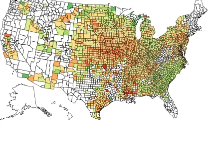
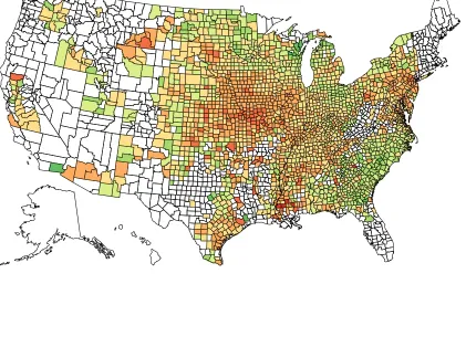
Figure 1.1 shows the assumed correlations for four different crops with revenue insurance available through the federal program. The Pearson correlations used in constructing premium rates for corn range from 0 in most states to -0.4 in Illinois and Iowa. The pattern of correlation follows, very roughly, the total quantities of corn that are produced in different states in the U.S. Figure 1.2 shows estimated Pearson correlations between yields and prices for all corn producing counties. The estimated correlations are similar to those assumed by RMA in states like Iowa and Illinois, but there are large differences in the South and along the Mississippi River. RMA assumes zero correlation in all counties in Mississippi, while counties near the Gulf of Mexico appear to have strong negative dependence.
A strange finding is positive Pearson correlation in many counties in eastern North Carolina, South Carolina, Minnesota, and Wisconsin. Similar positive relationships hold when dependence is measured using Spearman’s rho or Kendall’s tau as in Figures 1.3 and 1.4. There are several reasons why a given county could have yields that are positively dependent with respect to the Chicago Mercantile Exchange price. Instabilities in demand or supply could generate such results, and more broadly, the price formation process in Chicago is determined by many factors. The importance of any single county yield in determining the futures price is practically zero. The farther away the market implied by the revenue policy is from the ideal market underlying the theory of the natural hedge, the less likely the natural hedge is to hold.
Table 1.2: Frequencies of Selected Copulas
Number of Times Copula is Selected
Copula Frequency Percent
Normal 504 22.38
t 153 6.79
Gumbel 231 10.26
Clayton 268 11.90
Frank 641 28.46
Gumbel Rot. 455 20.20
Clayton Rot. 0 0.00
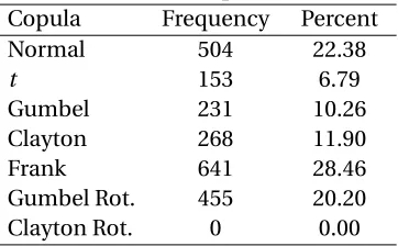
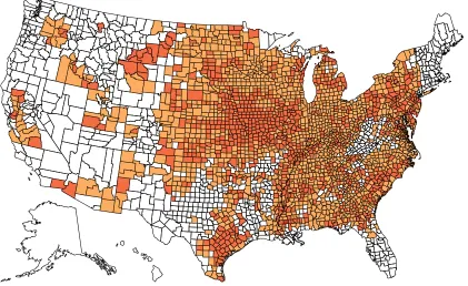
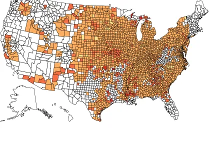
likelihood techniques. Normalized prices and yields were first converted to the uniform scale using the empirical distribution function. Then the copula portion of the likelihood was maximized over the uniform data. We estimate normal,t, Gumbel, Clayton, Frank, 90 degree rotated Gumbel, and 90 degree rotated Clayton copulas. The best fitting copula was selected according to Akaike Information Criteria (AIC). The selected copula in each county is shown in Figure 1.7, while the frequency of selection for each copula family is shown in Table 1.2.
Overall, there is a large amount of variation in the selected copula. In areas with negative dependence, the best fitting copula is usually either the Frank or normal copula. Areas with positive dependence are often best described with a Clayton ort copula. As data determining the direction of dependence also determine the strength of tail dependence and type of joint symmetry, geographic clustering is to be expected. Frank and Gaussian copulas are similar in terms of joint symmetry and tail dependence. However, an unrotated Clayton copula implies joint occurrence of low yields and low prices. Simultaneously low yields and prices result in the largest losses under a revenue insurance policy. We might expect that counties where the Clayton copula is selected will have higher premium rates as a result of this increased risk. Having shown that the copula models are grouped geographically, premium rates can be calculated under both the assumed dependence structure and the best fitting copulas.
procedure results in 1,000 simulated yields and prices for each copula model in each county. Using these sets of yields and prices, a distribution of revenue can be formed and losses under the artificial revenue policy can be obtained.
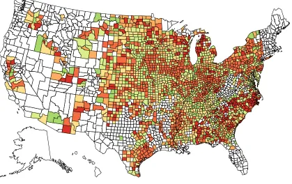
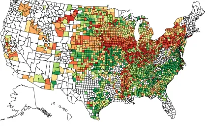
Figure 1.8 maps the difference in rates between models based on a Gaussian copula with data-driven correlation and a Gaussian copula with correlation according to Figure 1.1. The difference in rates resulting from misspecified correlation is small. A histogram and kernel density of the differences is shown in Figure 1.10. Rate differences are grouped about zero, although there are a few outliers. Even in the most extreme cases, differences in Pearson correlation only result in rate differences on the order of one or one and a half points. In spite of the small difference in rates, Figure 1.8 shows evidence of systematic variation across space. In counties where the estimated Pearson correlation is more negative than the RMA correlation, the difference is usually positive. In locations where the assumed correlation is more strongly negative, at least when compared to the estimated correlation, the difference in rates is often negative.
Figure 1.9 maps the difference in rates between the model based on the best fitting copula and the model with Gaussian copula and fixed correlation. The kernel density in Figure 1.11 shows that when the copula is allowed to vary along with strength of dependence, premium rates in many counties are higher than the rates under fixed correlation and a normal copula. This difference is largest in those counties where there is evidence of positive dependence and the Clayton copula is best fitting. The Clayton copula has lower tail dependence and a higher probability of obtaining low yields and low prices at the same time. For revenue insurance, such a scenario can be considered worst case. The clear spatial patterns exhibited in the data suggest that randomness does not drive these results.
Both county varying correlation and county varying copula models result in regular differences in the estimated price of insurance. In an absolute sense, the difference in premium rates resulting from misspecified correlation is small, while the error from a misspecified copula model is much larger. Of course, a change in the copula model naturally subsumes any change in correlation. The assumption of zero Pearson correlation between prices and yields, when combined with the Gaussian copula, is an exceptionally strong assumption. It further implies zero rank correlation and is equivalent to assuming that the relationship between prices and yields can be described with the independence copula. From Figure 1.1, independence is the underlying assumption in the majority of states for corn, soybeans, wheat, and cotton. In the case of cotton, no county is assumed to have any dependence between the county yield and the normalized price.
can lead to these types of profits. We would likely arrive at similar conclusions if we implemented a pooling scheme to combine similar copulas. The ability to accurately measure and describe depen-dence is thus relevant for public policy. Inaccurate measurement of dependepen-dence relationships can lead to large differences in premium rates and deviance from the actuarially fair premium.
1.5
Conclusion
Earlier work in crop insurance ratemaking has demonstrated that premium rates are sensitive to actuarial assumptions. It has also shown the effectiveness of adjusting for small samples by pooling information across space. These studies have generally confined themselves to crop yields so that any pooling only affects the marginal distribution of yields. Crop yields in areas that are closer to one another are more likely to be similar than yields in locations that are farther away. Spatial correlation results primarily from underlying weather, soil, and disease risks. Because perils are distributed across space, pooling data is a valid approach for pricing these types of insurance. Failure to account for spatial autocorrelation can lead to large variation in parameter estimates.
The results presented here show that dependence between yields and prices, or more generally the natural hedge, also clusters. Furthermore, this clustering is not limited to simple correlation, but extends to other aspects of the dependence structure. Counties that are close to one another tend to have similarities across several features of dependence and copula properties. After estimating a variety of copula models, the best fitting copula varies across counties. This implies variation in Archimedeanity, radial symmetry, and tail dependence.
We find that premium rates diverge from those calculated with fixed dependence structures. These differences in rates can lead to disparities in insurance demand, particularly if the underlying policy is not subsidized. If the natural hedge is not properly accounted for, premium rates will be too high or too low relative to the actuarially fair rate. Deviance in rates can result in problems of adverse selection and a lack of demand from the least risky farmers. Already faced with low elasticities of demand, the federal program would not be sustainable under such conditions. It is important to recognize that these differences in rates can only be generalized to policies with similar loss functions. Other types of insurance, such as revenue insurance with a harvest price option, will have different relationships between the joint distribution of revenue and the price of the policy.
Rho
-0.8 - -0.6
-0.6 - -0.4
-0.4 - -0.2
-0.2 - 0
0 - 0.2
0.2 - 0.4
0.4 - 0.6
0.6 - 0.8
Rho
-0.8 - -0.6
-0.6 - -0.4
-0.4 - -0.2
-0.2 - 0
0 - 0.2
0.2 - 0.4
0.4 - 0.6
0.6 - 0.8
Tau
-0.8 - -0.6
-0.6 - -0.4
-0.4 - -0.2
-0.2 - 0
0 - 0.2
0.2 - 0.4
0.4 - 0.6
0.6 - 0.8
D
-0.5 - -0.25
-0.25 - 0
0 - 0.25
0.25 - 0.5
DCorr
0 - 0.2
0.2 - 0.4
0.4 - 0.6
0.6 - 0.8
0.8 - 1
Copula
Clayton
Frank
Gumbel
Gumbel Rot.
Normal
t
Difference in Rates
-8.56069E-03 - -7.38492E-04
-7.35092E-04 - -3.05367E-04
-3.05239E-04 - -1.26174E-04
-1.25999E-04 - -2.93338E-05
-2.92502E-05 - 0.00000E+00
3.49252E-08 - 1.48992E-04
1.50918E-04 - 8.18676E-04
8.26723E-04 - 1.30348E-02
Figure 1.8: Difference in Premium Rates
Difference in Rates
-0.006208755 - -0.001047970
-0.001042801 - -0.000197383
-0.000190321 - 0.000891188
0.000897881 - 0.003109125
0.003110148 - 0.005324048
0.005335349 - 0.008474902
0.008478028 - 0.013015472
0.013058299 - 0.070348693
Figure 1.9: Difference in Premium Rates
-0.010 -0.005 0.000 0.005 0.010 0.015
Difference in Rates
0 25 50 75 100 125 150
P
e
rc
e
nt
Kernel
Figure 1.10: Histogram and Kernel Density of Rate Differences
0.00 0.02 0.04 0.06 0.08
Difference in Rates
0 10 20 30 40
P
e
rc
e
nt
Kernel
Figure 1.11: Histogram and Kernel Density of Rate Differences
CHAPTER
2
RATING EXOTIC PRICE COVERAGE IN
CROP REVENUE INSURANCE
Federal crop insurance has grown in size since the early 1990s and accounts for nearly nine percent of total five year projected spending under the Agricultural Act of 2014 (Congressional Budget Office, 2014). This is a significant portion of expected outlays as traditional agricultural programs encompass only twenty percent of total spending; remaining expenditures are marked for nutrition programs. Among the twenty-one different policies available through the federal crop insurance program, revenue insurance policies have played an increasingly important role. Revenue Protection (RP) and Revenue Protection-Harvest Price Exclusion (RP-HPE) insurance covered roughly seventy percent of the $101 billion total insured value in federal crop insurance for the 2015 crop year (Risk Management Agency, 2015).
a preference for the harvest price replacement feature and the additional coverage that this feature offers.
Because of the public-private nature of federal crop insurance, private companies that market and service insurance policies cannot compete on insurance offerings covered under the program. Proponents of government administrated crop insurance believe that overall liability in the program is too large for private markets to bear due to the spatially correlated and state dependent nature of agricultural risks (Miranda and Glauber, 1997). In spite of this perception, private insurers continue to furnish single peril agricultural insurance, as well as add-ons that provide flexibility around the policies available through the federal crop insurance program.
One dimension of the federal program that offers potential for more extensible private products is extended price coverage: the amount and type of price risk that insurance services indemnify. In the government program, price discovery for most major crops is determined using a planting time futures price (typically the February average price) of a harvest time futures contract (usually a November or December contract). However, a one-size-fits-all approach to establishing price guarantees may not align with the needs of individual producers. An insurance option that provides flexibility around this point involves establishing price coverage on the basis of an average or maximum of prices observed over a fixed interval. For example, one might envision coverage that establishes a revenue guarantee using the highest observed monthly average value of a futures contract for the months between January and May.
Additional price coverage can be offered by private insurers as an add-on to standard RP and RP-HPE policies or as a standalone policy. In the first case, farmers purchase an underlying revenue insurance policy through the federal crop insurance program. Supplemental exotic price coverage can then be purchased from a private provider at an additional premium. This type of pricing is similar to current RP policies where an additional premium is added to the RP-HPE rate to account for added price coverage.
Private insurers have an incentive to capture the business generated by federally subsidized insurance even though they cannot legally compete for this business in terms of the parameters of the underlying policies. An inclined way of attracting federal crop insurance customers to a particular insurer is for the insurer to offer private exotic price coverage in addition to the policies available through the federal program. Insurers with more desirable add-ons will be able to obtain a larger share of the federal program’s book of business.
of revenue policies offered by RMA, it is only necessary to consider a two-dimensional probability distribution. With recent advances in econometrics and statistics, it is possible to develop modeling methods that are tractable and possess the flexibility necessary to characterize the risks inherent in exotic price coverage options and policies.
There are a number of general approaches to measuring the risks associated with financial instruments based on averages or order statistics. Financial options on extrema are often termed exotic options. The pricing of such exotics is a growing area of financial research that requires the analyst to grapple with a number of dependencies. Zhang (1997) and Privault (2014) provide overviews of the pricing of exotic options under a set of basic assumptions. While Zhang (1997) approaches risk and pricing from a financial perspective, we use primarily statistical techniques to develop similar measures in the insurance context. Actuarial methods used in the federal crop insurance program are retained as much as possible, provided that they do not impose unreasonable assumptions in the course of the modeling exercise. This clarifies the connection between exotic price coverage and publicly offered policies. It also allows us to highlight the new or different strategies we employ in tackling major modeling issues.
Our basic approach is to consider average futures prices over individual months. This leads to a multivariate distribution with important dependencies among relative monthly average prices. The structure of this dependence varies by crop and is related to the evolution of the price of the underlying futures contract. Copula functions that capture tail dependence are used to model the joint distributions. Though we make some assumptions on the form of the copula for convenience, it is relatively easy to draw from a wide variety of copulas, and thus obtain a high degree of flexi-bility. Higher ordered but less flexible multivariate elliptical copulas are considered. Hierarchical Archimedean copulas (HACs) are a flexible alternative to elliptical copulas; they are capable of parsimoniously capturing asymmetric tail behavior.
2.1
Federal Crop Insurance and Revenue Coverage
Farmers have migrated toward the purchase of revenue insurance policies as federal crop insurance has become an increasingly important risk management tool. Traditional insurance against crop yield losses does not necessarily protect farmers from low prices. Though prices and yields are typically thought to have an inverse relationship, often termed the natural hedge, it is possible for simultaneous declines to occur. Revenue insurance provides the farmer with protection from falling yields and falling prices. The most recent Farm Bill expanded federal crop insurance by adding a new area-wide insurance program known as Stacked Income Protection (STAX) and a Supplementary Coverage Option (SCO).
The most widespread revenue insurance product is Revenue Protection (RP) insurance. The premium on RP policies is calculated using planting and harvest time futures prices. For example, the projected price for many corn policies is the February average price of a December futures contract. The realized harvest price is the October average price of the same December futures contract. RP has historically been offered for crops that have an active futures market. For most crops, price information is obtained from trading at the Chicago Mercantile Exchange. Daily volume on major crops, such as corn and soybeans, is typically well above 200 thousand contracts. RP offerings have occasionally been rescinded for crops with thinly traded futures markets such as rice.
RP and RP-HPE insurance are distinguished by the harvest price replacement feature. A loss occurs under RP-HPE if
YGPFλ >YHPO (2.1)
whereYG is the yield guarantee,PF is the price guarantee (planting time or February average price),
λ∈(0, 1)is the coverage level,YH is realized or harvest yield, andPO is the realized price (harvest
time or October average price).1In other words, a loss occurs when realized revenue (a function of
the harvest price) falls below guaranteed revenue (a function of the planting price).
With RP, guaranteed revenue is a function of both the harvest price and the projected price. The loss condition is
YGmax(PF,PO)λ >YHPO (2.2)
The maximum of the two prices (February and October) is used in constructing the revenue guaran-tee and thus determines losses and indemnities. Additional coverage under RP is largely intended to protect producers who contract their crop before harvest. If prices increase, but the farmer has a
yield shortfall, he will receive an indemnity payment that can be used to defray the purchases nec-essary to meet his contract obligations. While farmers who forward contract have obvious reasons for preferring the harvest price replacement feature, RP insurance purchases are not limited to this subset of farmers.
Several lines of reasoning may provide justification for the popularity of RP policies and serve to motivate our consideration of exotic price coverage. From a behavioral standpoint the purchase of insurance policies based on maxima are no regret. The farmer is paid at the best possible price over the interval. In the case of coverage that depends on an average of prices, the distributions of the averages may have favorable properties. The average of many independent and identically distributed random variables will have a smaller variance that the individual random variables themselves. Policies built around these averages could offer a cheaper way for farmers to insure against price risk. Du, Feng, and Hennessy (2017) found that crop insurance decisions are subject to behavioral anomalies. Regardless of the possibility of irrational purchase decisions, we do not characterize the farmer’s motivation any further; the preference of producers for additional coverage in the form of the harvest price replacement feature has been amply demonstrated in insurance markets.