Measuring the effect of commuting on the performance of the Bayesian Aerosol Release Detector

Open Access

Research

Measuring the effect of commuting on the performance of

the Bayesian Aerosol Release Detector

Aurel Cami*

_{, Garrick L Wallstrom}

_{and William R Hogan}

Address: 1_{Children's Hospital Boston Informatics Program, Boston, MA, USA and} 2_{Department of Biomedical Informatics, University of}

Pittsburgh, Pittsburgh, PA, USA

Email: Aurel Cami* - [email protected]; Garrick L Wallstrom - [email protected]; William R Hogan - [email protected] * Corresponding author

Abstract

Background: Early detection of outdoor aerosol releases of anthrax is an important problem. The Bayesian Aerosol Release Detector (BARD) is a system for detecting releases of aerosolized anthrax and characterizing them in terms of location, time and quantity. Modelling a population's exposure to aerosolized anthrax poses a number of challenges. A major difficulty is to accurately estimate the exposure level--the number of inhaled anthrax spores--of each individual in the exposed region. Partly, this difficulty stems from the lack of fine-grained data about the population under surveillance. To cope with this challenge, nearly all anthrax biosurveillance systems, including BARD, ignore the mobility of the population and assume that exposure to anthrax would occur at one's home administrative unit--an assumption that limits the fidelity of the model.

Methods: We employed commuting data provided by the U.S. Census Bureau to parameterize a commuting model. Then, we developed methods for integrating commuting into BARD's simulation and detection algorithms and conducted two studies to measure the effect. The first study (simulation study) was designed to assess how BARD's detection and characterization performance are impacted by incorporation of commuting in BARD's outbreak-simulation algorithm. The second study (detection study) was designed to measure the effect of incorporating commuting in BARD's outbreak-detection algorithm.

Results: We found that failing to account for commuting in detection (when commuting is present in simulation) leads to a deterioration in BARD's detection and characterization performance that is both statistically and practically significant. We found that a simplified approach to accounting for commuting in detection--simplified to maintain tractability of inference--nearly fully restored both detection and characterization performance of BARD detector.

Conclusion: We conclude that it is important to account for commuting (and mobility in general) in BARD's simulation algorithm. Further, the proposed method for incorporating commuting in BARD's detection algorithm can successfully perform the necessary correction in the detection algorithm, while preserving BARD's practicality. In our future work, we intend to further study the problem of the trade-off between running time and accuracy of the computation in BARD's version that includes commuting and ultimately find the best such trade-off.

from 2008 International Workshop on Biomedical and Health Informatics in conjunction with 2008 IEEE Conference of Bioinformatics and Biomedicine (BIBM)

Philadelphia, PA, USA. 3 November 2008

Published: 3 November 2009

BMC Medical Informatics and Decision Making 2009, 9(Suppl 1):S7 doi:10.1186/1472-6947-9-S1-S7

<supplement> <title> <p>2008 International Workshop on Biomedical and Health Informatics</p> </title> <editor>Illhoi Yoo and Min Song</editor> <note>Research</note> <url>http://www.biomedcentral.com/content/pdf/1472-6947-9-S1-info.pdf</url> </supplement>

This article is available from: http://www.biomedcentral.com/1472-6947/9/S1/S7

© 2009 Cami et al; licensee BioMed Central Ltd.

Introduction

Disease surveillance has a long history in Public Health. However, recent years have witnessed a sharp increase in the research devoted to the very early detection of disease outbreaks [1,2]. The diseases that have received special attention include those that occur naturally, especially the emerging infectious diseases, and those that may be caused by acts of bioterrorism. The detection of outbreaks is typically achieved through the analysis of various types of pre-diagnostic disease data, such as the counts of Emer-gency Department (ED) visits or the sales of over-the-counter healthcare products. To increase the utility of these data for detecting outbreaks of specific diseases, sur-veillance systems typically categorize the data according to various medical criteria. For example, the category of ED visits with influenza-like illness may be analyzed to detect influenza outbreaks. Similarly, the category of ED visits with respiratory chief complaints (RCC) may be analyzed to detect outbreaks of a respiratory disease, such as the

dis-ease caused by the inhalation of B. Anthracis spores. The

use of such pre-diagnostic and categorized data for the purpose of detecting disease outbreaks is sometimes

known as syndromic surveillance.

The early detection of outdoor aerosol releases of anthrax is an important problem because a release could infect hundreds of thousands of individuals and without early detection mortality could be as high as 30,000 to 3 mil-lion [3]. Further, the accurate characterization of an aero-sol release in terms of time, location and quantity might assist responders in mitigating the impact of an outbreak. The Bayesian Aerosol Release Detector (BARD) is a system for detecting and characterizing releases of aerosolized anthrax. BARD integrates the analysis of biosurveillance data (counts of ED visits with RCC), meteorological data and geographical data. Through this analysis BARD attempts to determine whether the current spatio-tempo-ral pattern of respiratory disease incidence in a region is more consistent with the historical patterns or with the pattern that BARD would expect with an aerosol anthrax release.

Modelling a population's exposure to aerosolized anthrax poses a number of challenges. A major difficulty is to accurately estimate the exposure level--the number of inhaled anthrax spores--of each individual in the exposed region. A key determinant of the exposure level of an indi-vidual is his/her spatial location at the time of exposure. Hence, to accurately estimate the exposure level it would be desirable to perform a fine-grained spatial modelling at the person-level. However, the data needed to parameter-ize such models are difficult to obtain. In fact, the only type of spatial information that is typically contained in biosurveillance databases is the home administrative unit--such as the home zip code--of each patient. To deal

with this challenge posed by the lack of fine-grained spa-tial data, nearly all anthrax biosurveillance systems, including BARD, make two simplifying assumptions. First, they assume that all individuals who live in the same administrative unit would have the same exposure level--typically taken to be the level at the unit's centroid. Sec-ond, they assume that exposure to anthrax would occur at one's home administrative unit. Whether it is possible to relax the first assumption remains currently an open prob-lem. On the other hand, in the last few years there has been some progress toward relaxing the second assump-tion. The key to this progress has been to integrate biosur-veillance systems with mobility models that are parameterized through data that describe the travel pat-terns of the population. For one type of travel, namely the work-related commuting, such datasets are publicly avail-able from the U.S. Census Bureau. For other types of travel, data are more difficult to obtain.

The first study that incorporated a mobility model in the simulation of anthrax outbreaks was conducted by Buck-eridge [4]. He developed methods for integrating mobility in outbreak simulation and employed commuting data provided by the U.S. Census Bureau as well as survey based, non-commuting travel data. Then, he investigated the impact that incorporation of mobility in outbreak simulation had on two outbreak detection algorithms: a cumulative-sum temporal algorithm [1,2] and the SMART spatial algorithm [5]. A few other papers have investigated incorporation of mobility in biosurveillance. Duczmal and Buckeridge [6] proposed a method for integrating a commuting model with Kulldorf's spatial scan algorithm [7]. Garman et al. [8] developed a method for probabilis-tically inferring the work zip code from the home zip code and then integrated this method with the PANDA detec-tion algorithm [9]. Cami et al. [10] developed a method for integrating commuting with BARD detection algo-rithm.

This paper describes a method for incorporating commut-ing into BARD. First, we incorporate commutcommut-ing into BARD's outbreak-simulation algorithm. Then, we present the results of an experimental study that assessed how BARD's detection and characterization performance are impacted as a result. Next, we present the results of a sec-ond study designed to measure the effect of incorporating

commuting in outbreak detection. Finally, we compare the

results of the simulation and detection studies, discuss the findings and limitations of this work and outline some directions for future research.

Background

A brief description of BARD

To simplify our exposition, we follow the terminology in Lawson and Kleinman [1] and generically refer to the basic administrative spatial units employed for aggregat-ing the disease data (e.g., block groups or zip codes) as

tracts. The main symbols used in this paper and their respective meanings are listed in Table 1.

BARD detector

BARD detector attempts to discriminate between two hypotheses. The null hypothesis states that only "back-ground" respiratory disease is present in the surveillance region. The alternative hypothesis states that both back-ground respiratory disease and a respiratory disease caused by an aerosol release of anthrax are present. Using Bayes' theorem, BARD computes the posterior probability

of the attack hypothesis H₁ given data, as follows:

In addition, BARD computes the likelihood ratio, or the Bayes' factor

In equations (1)-(2), b is the biosurveillance vector

consist-ing of the tract-level counts of ED visits with RCC durconsist-ing

the last 24 hours; G is the geographical matrix containing

the tract populations and the x, y coordinates of the tract

centroids; M is the meteorological matrix containing the

wind speed, the wind direction and the atmospheric sta-bility class--a measure of atmospheric turbulence--for var-ious observation times during the most recent week. The

posterior probability of H₁ and the Bayes' factor are both

measures of the evidence provided by the data in favour of the alternative hypothesis.

The two key quantities in equations (1)-(2) are P(b|H₀, G,

M), the likelihood of biosurveillance data under H₀, and

P(b|H₁, G, M), the likelihood of biosurveillance data

under H1. Assuming conditional independence among

the counts of different tracts given a hypothesis and the meteorological conditions, BARD computes the two

region-wide likelihoods P(b|H₀, G, M) and P(b|H₁, G, M)

by first computing the corresponding tract-level likeli-hoods and then using equations:

In eq. (3), c_i denotes the 24-hr count of tract i and r =(x, y,

h, q, t) denotes the release parameter vector, consisting of

the release location x, y, h, the release quantity q, and the

release time t. To compute the tract-level likelihoods P(c_i

|H₀, G, M) and P(c_i |H₁, G, M, r), BARD employs the

bino-mial probability model (see [3,10] for more details). Finally, BARD performs the integration over the release

scenarios r through a Monte Carlo integration technique

called likelihood weighting [3].

In addition to computing the two detection statistics

dis-cussed above--the posterior probability of H₁ and the

Bayes' factor--BARD attempts to characterize a release by computing an estimate for each element of the release

vec-tor r. The estimation of r is carried out in Bayesian

fash-P H P H P H

P _{Hi P Hi} i

( | , , ) ( | , , ) ( )

( | , , ) ( )

,

.

1 1 1

0 1

b G M b G M

b G M

= =∑

(1)

P H P H

( | , , )

( | , , ).

b G M

b G M

1 0

(2)

P H P c H

P H P c H

i i

i i

( | , , ) ( | , , ),

( | , , ) ( | , , , )

b G M G M

b G M G M r

0 0

1 1

=

= ⎡

⎣ ⎢

∏

∏

⎢⎢

⎤

⎦ ⎥ ⎥

∫

r

1

(3)

Table 1: List of symbols

Symbol Meaning

t release date and time

x, y, h, release coordinates

q release quantity

ni population of tract i

c_i number of cases who live in tract i

d_i dose of spores in the centroid of tract i

θi ED-visit probability of each individual who lives in tract i, given that a release has occurred and assuming that commuting has not taken

place

G commuting graph: nodes denote tracts, arcs denote commuting flows

n_ij for i ≠j, number of people who live in tract i and work in tract j; for i = j, number of people who live in tract i and who either don't work

or work in tract i

cij for i ≠j, number of cases who live in tract i and work in tract j; for i = j, number of cases who live in tract i and who either don't work or

work in tract i

Out (i) union of set {i} with the set of all tracts where people who live in tract i work

ED-visit probability of each individual who lives in tract i, given that a release has occurred and assuming that commuting has taken place

ion. BARD assumes that the release parameters are

conditionally independent given H₁, i.e.,

BARD employs a uniform prior for each element of r,

except h, for which a prior that favours smaller release

heights relative to the higher ones is employed (see [3], p. 5248). Finally, BARD computes the posterior expectation

of each element of r inside the likelihood-weighting

inte-gration procedure. The posterior expectation of r

consti-tutes the release characterization produced by BARD.

BARD simulator

BARD can also simulate outbreaks of the respiratory dis-ease caused by an aerosol reldis-ease of anthrax. Algorithm 1 gives a high-level description of BARD's outbreak simula-tion algorithm.

Algorithm 1: BARD outbreak simulation

input: surveillance region, release date/time, location, and quantity

output: list of simulated cases for each tract of surveillance region

foreach tract i of surveillance region do

1. compute the dose of spores di in the centroid of tract i

using the Gaussian plume model (see [3])

2. compute the probability θ_i that an individual who lives

in tract i will visit an ED, given the dose of spores d_i (see

[3])

3. generate the number of cases c_i for tract i by drawing a

random variate from Bin(ni, θi), where ni is the population

of tract i

4. foreach case of tract i do

a. draw a random time interval from a lognormal

distri-bution corresponding to the dose d_i (see [3])

b. add this interval to the release date/time to obtain the time of ED visit for this case

end

end

For brevity, in Algorithm 1 we have left out a number of details that are not necessary for understanding the flow of the computation. These details can be found in [3].

Methods

Biosurveillance data

Our disease data--counts of ED visits with RCC--corre-spond to a region surrounding the city of Pittsburgh. This region consists of seven counties: Allegheny, Armstrong, Beaver, Butler, Lawrence, Washington, and Westmore-land. The historical ED data for our experiments were pro-vided by 10 EDs operated by one health system. These data represented nearly 30% of all ED visits in the surveil-lance region. We divided the total period spanned by the available ED data into a training period (1 January 1999 to 31 December 2004), which was used to train BARD's detection algorithm, and a test period (1 January 2005 to 31 December 2005), used in our evaluation experiments. Finally, the weather data were provided from the National Weather Service, while the populations and central zip codes came from the ESRI ArcGIS Desktop product.

Data and model for commuting flows

The data that describe the commuting patterns were pro-vided by the U.S. Census Bureau. These data were col-lected during the 2000 Census, have national coverage

and are provided at the census tract level: each commuting

flow denotes the average daily number of commuters between a home census tract and a work census tract. The commuting flows can be naturally modelled by a weighted, directed graph in which nodes denote tracts, arcs represent commuting flows, and the weight of an arc denotes the number of commuters in the corresponding flow. We extracted from the nationwide commuting data-set the commuting flows for which both the residence tract and the work tract belong to our surveillance region. The total number of commuters in this intra-region subset of flows was 1,005,566.

As a pre-processing step, we needed to transform the com-muting flows from the census tract level provided by the U. S. Census Bureau to one of the two levels supported by the BARD simulator: zip code, or block group. In this paper we performed the latter transformation mainly because the block-group level is finer-grained than the zip-code level and thus has the potential to lead to a more accurate estimation of the release location by BARD. Note that block group is a sub-unit of census tract (i.e., each census tract is partitioned into two or more block groups). To perform the desired transformation, we split each

com-muting flow between a pair of census tracts T₁, T₂ into

sev-eral smaller-sized flows according to the following two intuitive rules: (i) the number of workers coming from

each constituent block group of T₁ was assumed to be

pro-portional to the block group population; (ii) the number

of workers going to T₂ was assumed to be evenly divided among its constituent block groups. The final commuting graph for our region consisted of 1991 nodes (block groups) and 324,402 arcs (commuting flows).

Integration of commuting with BARD simulator

We refer to the version of BARD simulator that takes com-muting into account as the BARD-C simulator. BARD-C simulator takes as input a representation of the

commut-ing graph G, in addition to the surveillance region and the

anthrax release parameters. The key observation employed in the incorporation of commuting in simula-tion is that if a release occurs during working hours, a worker would be exposed at the dosage level correspond-ing to his/her work tract rather than the dosage level of his/her home tract. This idea is implemented in BARD-C by modifying the Step 3 of Algorithm 1, namely the com-putation of the ED-visit count for each tract. To realize this modification BARD-C first computes the ED-visit count corresponding to each commuting flow separately and then re-aggregates the workflow-level counts according to the home tract. More precisely, the number of cases for

each tract i is computed as

where

In eqs. (5)-(6), c_i denotes the total number of cases who

live in tract i, Out(i) ={i} ∪ {j|(i, j) is an arc of G} denotes

the union of set {i} with the set of out-neighbours of tract

i in the commuting graph G (i.e., the tracts where people

living in tract i go to work), n_ij, i ≠j, denotes the weight of

the arc (i, j) in the graph G, i.e., the number of people

liv-ing in tract i and working in tract j, and n_ii denotes number

of people who either don't work, or who both live and

work in tract i. Finally, c_ij, i ≠ j, denotes the number of

cases who live in tract i and work in tract j, c_ii denotes

number of cases who either don't work, or who both live

and work in tract i and θ_j denotes the probability that a

person who is exposed in tract j will visit an ED, given that

a release has occurred.

This refined computation of the tract-level ED counts in BARD-C could alternatively be implemented by modify-ing the ED-visit probability of each individual who lives

in tract i (i.e., modifying the Step 2 of Algorithm 1) prior

to generating the number of cases for tract i as a binomial

random variate. Indeed, let us denote by the

probabil-ity that an individual who lives in tract i will visit an ED,

given that a release has occurred and assuming that

com-muting has taken place. Let the parameter θ_i denote, as

before, the probability that an individual who is exposed to

anthrax in tract i will visit an ED. By approximating the binomial distribution with a Poisson distribution and recalling that the sum of independent Poisson random variables is also a Poisson random variable, it is straight-forward to show that the method for generating the count

c_i specified by eqs. (5)-(6) is essentially the same as

gener-ating the count ci from a binomial distribution Bin(ni,

), where

The above two methods for incorporating commuting in simulation differ slightly from the method employed by Buckeridge [4]. In [4], other non-commuting types of mobility were also taken into account and therefore the exposure tract could be different from both the residential and the work tract. Hence, in [4] the incorporation of mobility was based on the computation of conditional

probabilities P(exposed in tract i|t, live in tract j) for all

pairs i, j.

After generating the number of cases for each tract, BARD-C computes the ED-visit time of each simulated case by, again, taking into account the fact that a worker would be exposed at the dosage level of his/her work tract. This idea is implemented in BARD-C by ensuring that in the Step 4(a) of Algorithm 1 the time of ED visit for a worker case is computed as a random deviate from the lognormal dis-tribution that corresponds to the dosage level at his/her work tract.

The incorporation of commuting in simulation leads to an increase in the running time of the Step 3 of BARD's simulation algorithm by a constant factor. It is straightfor-ward to see that this factor equals the average out-degree of the commuting graph. For the block group-level com-muting graph of the Pittsburgh region that we created, the average out-degree is nearly 150. However, the factor by which the total running time of BARD simulator is increased due to the incorporation of commuting is smaller. The reason for this is that Step 3 accounts for only a fraction of the running time of BARD. In a computer with a 3 GHz processor and 2 GB of main memory, a sim-ulation for the Pittsburgh region took nearly 2 minutes with BARD and nearly 20 minutes with BARD-C.

Verification of the correctness of simulation with commuting

To verify that BARD-C simulator works as intended, we generated a random release parameter vector, consisting

ci cij j Out i

=

∈

∑

,

( )

(5)

c_ij~Bin n( _ij,θ_j). (6)

θ_i∗

θ_i∗

θ_i θ_j

j Out i

nij ni

∗

∈

=

∑

( )

of the release time, location, and quantity. Then, using this fixed release parameter vector we produced 10 syn-thetic outbreaks with BARD-C simulator. Next, for each

tract i of the surveillance region, we fit a binomial model

Bin(n_i, ) to the sample of simulated counts .

As before, n_i denotes the known population of tract i, and

denotes the probability that an individual who lives in

tract i will visit an ED, given that a release has occurred and assuming that commuting has taken place. We denote

by the estimate of the binomial probability parameter

learned from the count data generated with BARD-C

simulator. Finally, we computed an analytical prediction

for each parameter . We achieved this by first using the

BARD simulator to compute the binomial probability

parameters θ_j for all j ∈ Out(i) and then computing the

analytical prediction of the parameter through eq. (7).

Integration of commuting model with BARD detector

We have also developed a method for integrating com-muting with BARD detector. A thorough discussion of this method is given [10]. We refer to the version of BARD detector that takes commuting into account as the BARD-C detector.

Measuring the impact of commuting in BARD's performance: simulation study

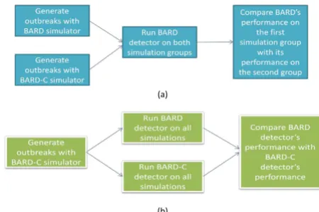
We conducted an experiment to measure whether BARD's detection and characterization performance is signifi-cantly affected by the incorporation of commuting in out-break simulation. In the remainder of the paper, we refer to this experiment as the "simulation study" because the emphasis of this study was on the integration of commut-ing with BARD simulator. In the next section we discuss a second study, where the emphasis is on the integration of commuting with BARD detector. We refer to this second study as the "detection study". Figure 1 illustrates the dif-ference between the objectives of the simulation and detection studies.

The simulation study followed a matched-pairs design.

First, a set of 185 release parameter vectors r = (t, x, y, h, q)

was generated. For all parameter vectors, the quantity q

was fixed at 0.5 kg. The release time t was chosen

uni-formly at random from the test period, i.e., the year 2005.

The parameters x and y where chosen uniformly at

ran-dom from a circular sub-region of the surveillance region centred in the city of Pittsburgh and having a radius of 40 km; this sub-region was found to have better ED-data

cov-erage than the whole region. Finally, the height h was

cho-sen from a non-uniform distribution that favours lower release heights relative to the higher ones.

We supplied each release vector r_i, i = 1,...,185, as input to

the BARD and BARD-C simulators. By doing so, we obtained one group of 185 simulations that did not take commuting into account and another group of 185 simu-lations that took commuting into account. We refer to

these two simulation groups as non-commuting and

com-muting, respectively. The synthetic cases generated in each simulation were injected into the real ED data from 2005. Next, each of the 370 semi-synthetic outbreaks was sup-plied as input to the BARD detector and its average per-formance over the non-commuting outbreak group was compared with its average performance over the commut-ing outbreak group.

BARD's detection performance was measured through the

time-to-detection--or timeliness--and its characterization

performance was measured through the t, x, y, h, and q

(absolute) errors. Each of the above six metrics is a function

of the alarm threshold, i.e., the threshold of the alarm

sta-tistic employed by BARD detector to discriminate between the non-outbreak and outbreak situations. For a given threshold, an alarm is considered to be false if the alarm statistic exceeds the threshold prior to the outbreak onset. The false alarm rate (for a given alarm threshold) is the number of false alarms that occur per unit of time. We measured it as the number of false alarms per year.

We employed two methods to compare BARD's perform-ance over the non-commuting group with its performperform-ance over the commuting group. The first method was Activity Monitoring Operating Characteristic (AMOC) analysis

θ_i∗ _{c c}

i i

1 10

,…,

θ_i∗

ˆ

θ_i∗

θ_i∗

θ_i∗

θ_i∗

Schematic representation of the simulation and detection studies

Figure 1

Schematic representation of the simulation and detection studies. Part (a): simulation study; part (b): detec-tion study

(a)

[11]. The AMOC curve of a performance metric (e.g., time-liness) plots the false alarm rate against that metric. The initial step in constructing an AMOC curve is to compute the alarm thresholds corresponding to various false alarm rates (in our case, 1 per year to 36 per year). We computed the alarm thresholds by running BARD detector on the baseline ED data for 2005. Next, these thresholds were

employed to identify the pairs of values of the form <false

alarm rate, performance metric> that constitute an AMOC curve. For each simulation group, we constructed a single AMOC curve per metric by plotting the false alarm rate

against the mean value of the given metric over the whole

simulation group.

The second method we employed to compare BARD's formance over the non-commuting group with its per-formance over the commuting group was statistical testing. Our null hypothesis asserted that for a given false alarm rate and performance metric, the mean of the given metric over the non-commuting group was equal to its mean over the commuting group. Testing was carried out

through the paired t test.

Comparing the performance of BARD and BARD-C detectors: detection study

We performed a second experiment designed to compare

the performance of BARD and BARD-C detectors over a set

of simulations generated with BARD-C simulator. As mentioned earlier, we refer to this experiment as the "detection study". Here, we briefly outline the design of this study; a full discussion is given in [10]. A total of 100 semi-synthetic outbreaks were generated using the

BARD-C simulator. For all simulations, the quantity q was fixed

at 0.5 kg. The release time t was chosen uniformly at

ran-dom from the test period, i.e., the year 2005. The

param-eters x, y, and h were drawn from their prior distributions.

Each semi-synthetic outbreak was supplied as input to the BARD and BARD-C detectors. The detectors were executed 42 times on each simulation in increments of 4 hours: the first execution began 4 hours after the release, the second execution 8 hours after the release, and so on.

The detection performance of both detectors was measured

through timeliness. AMOC analysis and statistical testing

were employed to compare the performance of the two

detectors. The characterization performance of both

detec-tors was measured through t, x, y, h, and q (absolute) errors.

Each characterization metric was plotted against the time interval from the release of anthrax to the beginning of the

detector's execution, which we call the time-to-execution.

Finally, a Wilcoxon signed ranked test was performed with respect to each characterization error.

Results

Correctness of simulation with commuting

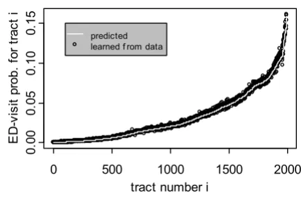
Figure 2 shows the results of our experimental verification of the correctness of simulation with commuting. This

fig-ure plots the estimated parameter values and the

ana-lytically predicted values for the 1991 tracts of our

surveillance region. The solid line corresponds to the pre-dicted values, while the points correspond to the values estimated from the simulated data. As shown, the pre-dicted values are in good agreement with the values esti-mated from the simulated data, indicating that BARD-C simulator works as specified.

Results of the simulation study

Figure 3 shows the daily mean number of cases (i.e., the epidemic curves) for the non-commuting and commuting simulation groups. In this figure, the horizontal axis shows the outbreak day, while the vertical axis shows the daily mean number of cases in the surveillance region. It can be observed that the shapes of these two curves are very similar. In particular, the two curves are seemingly identical at least up to the third outbreak day--the day when BARD typically detects a semi-synthetic outbreak. These two curves differ mainly around the peak of the out-break, where the commuting curve is slightly more ele-vated than the non-commuting curve. These observations imply that any differences between BARD detector's per-formance over one simulation group and its perper-formance over the second group could be attributed only to the change in the spatial distribution of cases caused by com-muting and not to a consistent discrepancy between the

ˆ

θ_i∗

θ_i∗

Verification of the correctness of simulation with commuting

Figure 2

Verification of the correctness of simulation with commuting. Plot of the analytically predicted values of ED-visit probability against the values estimated from data gener-ated with the BARD-C simulator

0 500 1000 1500 2000

0.

00

0.

05

0.

10

0

.15

tract number i

E

D

-v

is

it

p

ro

b

.

fo

r

tr

a

c

t i

sizes of outbreaks simulated with and without commut-ing.

With respect to q and h errors, we found that BARD's

per-formance over the non-commuting group was almost indistinguishable from its performance over the commut-ing group. Unexpectedly, the posterior mean of the release

parameters q and h did not appear to converge. We leave

the investigation of this unexpected outcome as a topic for future research and in the remainder of this section we focus only on the remaining four metrics.

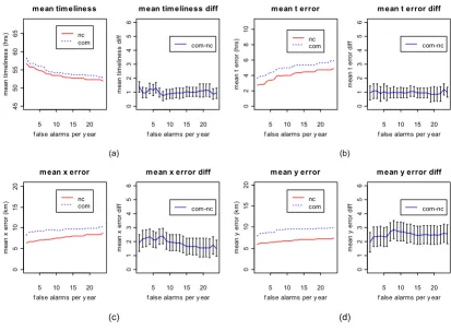
Figure 4 shows the results of the AMOC analysis for the

timeliness, t error, x error, and y error. As shown, in Figure

4(a), BARD's mean timeliness over the commuting group is nearly one hour greater than its mean timeliness over the non-commuting group, at each false alarm rate.

Like-wise, BARD's mean t error (Figure 4(b)) over the

commut-ing group is nearly one hour greater than its mean t error

over the non-commuting group, at each false alarm rate.

BARD's mean x and y errors (Figure 4(c-d)) on the

com-AMOC analysis for the simulation study

Figure 4

AMOC analysis for the simulation study. AMOC curves for (a) mean timeliness, (b) mean t error, (c) mean x error, and (d) mean y error. In each of the parts (a)-(d), the left panel shows the AMOC curves corresponding to the commuting (com) and non-commuting (nc) simulation groups, respectively, while the right panel shows the difference between commuting and non-commuting AMOC curves along with the error bars (plus/minus one standard error) for this difference

(a) (b)

(c) (d)

5 10 15 20

45

50

55

60

65

m ean tim eliness

f alse alarms per y ear

me a n ti me lin e s s (h rs ) _nc com

5 10 15 20

0

123456

m ean tim eliness diff

f alse alarms per y ear

m e an t im e lin es s dif f com-nc

5 10 15 20

0

2468

1

0

m ean t error

f alse alarms per y ear

m e a n t er ro r (h rs ) nc com

5 10 15 20

0

123456

m ean t error diff

f alse alarms per y ear

m e a n t er ro r dif f com-nc

5 10 15 20

0

5

10

15

20

m ean x error

f alse alarms per y ear

m e a n x er ro r (k m ) nc com

5 10 15 20

0123456

m ean x error diff

f alse alarms per y ear

m e an x er ro r dif f com-nc

5 10 15 20

0 5 1 0 15 20

m ean y error

f alse alarms per y ear

m e a n y er ro r (k m ) nc com

5 10 15 20

0123456

m ean y error diff

f alse alarms per y ear

m e an y er ro r dif f com-nc

ED visit counts generated with BARD and BARD-C simula-tors

Figure 3

ED visit counts generated with BARD and BARD-C simulators. Daily mean number of ED visits in the surveil-lance region for the non-commuting (nc) and commuting (com) simulation groups

0 5 10 15 20 25

muting group are each nearly 2 km greater than the respective mean errors on the non-commuting group.

Finally, Table 2 gives for all false alarm rates between 1 per year and 12 per year the p-values of the test for equal

means of BARD's timeliness, x error, y error, and h error

over the two simulation groups. From the results shown in Table 2 it can be concluded that, at each shown false

alarm rate, the mean timeliness, x error, and y error over

the non-commuting group are statistically different from the respective means over the commuting group, at the

0.05 significance level. The same holds for the t error with

the exception of three false alarm rates: 1, 4, and 6.

Results of the detection study

Some of the results appearing in this section (Figs 5 and 6) have been previously reported in [10]. We have

repro-duced these results here to contrast the simulation study with the detection study. This section also presents two new plots (Figs 7, 8) that correspond to our detection study but do not appear in [10]. Figure 5 shows the AMOC analysis for the timeliness of BARD and BARD-C detec-tors. As seen, BARD-C's timeliness is more than one hour smaller than BARD's timeliness at every false alarm rate. A

paired t test showed that, for each false alarm rate, the

mean timeliness of BARD-C was statistically different from the mean timeliness of BARD, at the 0.05 signifi-cance level.

Next, we turn to the characterization performance of BARD and BARD-C detectors. As in the simulation study, we found that the posterior means of the release

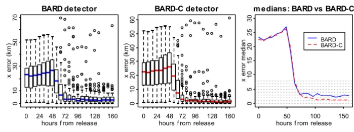
parame-Analysis of the characterization performance for the x error

Figure 6

Analysis of the characterization performance for the x error. Box plots and plot of the medians of the x error for BARD and BARD-C detectors

0 24 48 72 96 128 160

01

0

3

0

5

0

7

0 BARD detector

hours f rom release

x

err

or (k

m

)

0 24 48 72 96 128 160

0

1

02

0

3

0

4

05

0

6

0

BARD-C detector

hours f rom release

x

err

or (k

m

)

0 50 100 150

0

5

10

15

20

25

30

m edians: BARD vs BARD-C

hours f rom release

x

erro

r m

edian

BARD BARD-C Table 2: Results of the test for equality of BARD's errors over

the two simulation groups.

timeliness t error x error y error

far = 1 0.00014 0.06698 0.00139 0.0055

far = 2 0.00889 0.04066 0.00026 0.00106

far = 3 0.00991 0.03827 0.00024 0.00107

far = 4 0.00074 0.09732 0.00006 0.00061

far = 5 0.0046 0.04967 0.00017 0.00086

far = 6 0.00044 0.07566 0.0002 0.00068

far = 7 0.0041 0.01017 0.00004 0.00008

far = 8 0.03221 0.01087 0.00003 0.00003

far = 9 0.01664 0.00879 0.00059 0.00006

far = 10 0.01007 0.00689 0.00104 0.00006

far = 11 0.00819 0.00762 0.00107 0.00007

far = 12 0.00477 0.00775 0.00124 0.00013

The p-values of the test H₀: mean(metric) non-commuting equals

mean(metric) commuting--where metric can be timeliness, t error, x error, or y error.

AMOC analysis for the detection study

Figure 5

AMOC analysis for the detection study. AMOC curves for the mean timeliness of BARD and BARD-C detectors measured over a group of simulations generated with BARD-C simulator

0 5 10 15 20 25 30 35

4

5

60

75

timeliness AMOCs

false alarms per year

me

a

n

t

ime

lin

e

s

s

(

h

rs

)

ters q and h did not appear to converge as the time to exe-cution increased.

Hence, in the remainder of this section we focus on the x,

y, and t errors. Figure 6 shows box plots and plots of the

medians of the x error for BARD and BARD-C. In each plot

the horizontal axis shows the time-to-execution. The sam-ples from which the box plots were constructed corre-spond to the different simulations. Several conclusions

can be derived from Figure 6. First, the x error of both

BARD and BARD-C converges to relatively small values as

the time-to-execution increases. Second, the errors of BARD and BARD-C appear to converge around the same time and nearly 10-16 hours after the detection. Third, the

sampling distribution of the x error is right-skewed for

both detectors and in almost each execution of BARD and BARD-C there is a small number of outliers. Fourth, after

the convergence, the median of the x error for BARD-C is

nearly 2 km smaller than the median of the x error for

BARD.

Figure 7 plots the median of the y error for BARD and

BARD-C. The post-convergence median of the y error for

BARD-C was nearly 0.5 km smaller than the median for

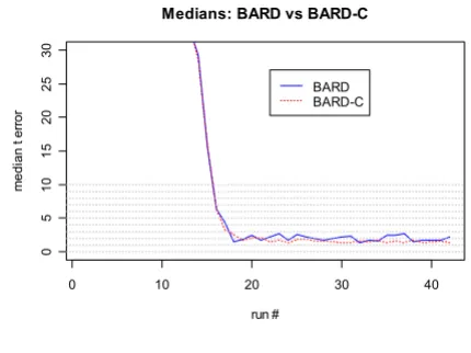
BARD. Finally, Figure 8 plots the median of the t error for

BARD and BARD-C. The post-convergence difference of

the medians for the t error was nearly 20 minutes.

Finally, we performed a Wilcoxon signed rank test whose null hypothesis asserted that BARD and BARD-C have

identical locations of the distributions of x error, y error,

and t error. The results of this test showed that after the

convergence of the x error, the p-values of the test remain

well below the 0.05 significance level (see [10]). Similar

comments can be made for the y error. For the t error the

convergence of the p values is not as clear as for the x and

y errors.

Conclusion

We incorporated commuting into BARD's simulation and detection algorithms and conducted two experimental studies to evaluate the effect. Incorporation of commuting in simulation is important to improve the fidelity of semi-synthetic outbreaks that BARD generates. Likewise, by incorporating commuting in detection we expect that the laboratory performance of the BARD detector would be closer to a real-world performance.

The results of our simulation study showed that incorpo-ration of commuting in outbreak simulation leads to a statistically significant deterioration in BARD's detection and characterization performance, when BARD's detec-tion algorithm does not account for commuting. Intui-tively, this result was expected since incorporation of commuting in simulation causes the spatio-temporal pat-tern of respiratory disease incidence to be different from the pattern BARD would expect under the alternative hypothesis. However, our precise quantification of the deterioration in BARD's performance due to commuting showed that this deterioration is practically significant. Indeed, BARD's timeliness increased by nearly one hour and based on previous estimates [12] that a delay of one hour in detection results in as much as $250 million addi-tional economic costs, this increase is quite significant.

Likewise, the t, x, y errors increased by nearly 30%, which

can also be considered a significant deterioration.

Analysis of characterization performance for the t error

Figure 8

Analysis of characterization performance for the t error. Plot of the median of the t error for BARD and BARD-C detectors

0 10 20 30 40

0

5

10

1

5

20

2

5

30

Medians: BARD vs BARD-C

run #

m

e

di

an

t er

ro

r

BARD BARD-C

Analysis of the characterization performance for the y error

Figure 7

Analysis of the characterization performance for the y error. Plot of the median of the y error for BARD and BARD-C detectors

0 10 20 30 40

0

5

10

1

5

20

2

5

30

Medians: BARD vs BARD-C

run #

m

e

d

ian y e

rr

o

r

Publish with BioMed Central and every scientist can read your work free of charge "BioMed Central will be the most significant development for disseminating the results of biomedical researc h in our lifetime."

Sir Paul Nurse, Cancer Research UK

Your research papers will be:

available free of charge to the entire biomedical community

peer reviewed and published immediately upon acceptance

cited in PubMed and archived on PubMed Central

yours — you keep the copyright

Submit your manuscript here:

http://www.biomedcentral.com/info/publishing_adv.asp

BioMedcentral

Our detection study showed that incorporation of com-muting in detection almost fully restores BARD's perform-ance in the sense that the performperform-ance of BARD-C detector on simulations produced with the BARD-C sim-ulator is close to the performance of BARD detector on simulations produced with BARD simulator.

Although others have measured the effect of population mobility on outbreak-detection performance, to our knowledge our work is the first to report the effect on out-break-characterization performance. We found that fail-ing to account for commutfail-ing in detection (when commuting is present in simulation) worsens characteri-zation performance. We found that our simplified approach to accounting for commuting in detection--sim-plified to maintain tractability of inference--significantly improved characterization performance over characteriza-tion without commuting.

Finally, we discuss the main limitations of our work. First, in creating the commuting graph of the surveillance region, we employed intuitive but arbitrary rules to trans-form the commuting flows into a spatial resolution sup-ported by BARD. The need for transforming the commuting flows could be avoided in the future by extending BARD so that it supports the census tract mode, but at the expense of coarser spatial granularity. Second, although we did not use the same commuting graph in both simulation and detection (see [10] for the details of how we truncated and sorted the commuting graph in detection mode) our studies did not perform a full sensi-tivity analysis with respect to the commuting graph. In our future work we plan to create a number of commuting graphs, each obtained by introducing random noise to the commuting data provided by the Census Bureau. Then, we will simulate several synthetic outbreaks with each of these noisy graphs and will compare BARD and BARD-C detectors over the whole range of simulations. Finally, as elaborated in [10], to bound the running time of the BARD-C detector, we made a number of simplifications at the expense of the accuracy of the computation. In our future work, we intend to further study the problem of the trade-off between running time and the accuracy of the computation in BARD-C detector and ultimately find the best such trade-off.

Competing interests

The authors declare that they have no competing interests.

Authors' contributions

AC, GLW and WRH developed the proposed methods, designed the experimental studies and prepared the man-uscript. AC implemented the proposed methods and per-formed the experiments.

Acknowledgements

This work was supported by the Centers for Disease Control and Preven-tion (CDC) under grant R01PH000026-01.

This article has been published as part of BMC Medical Informatics and Deci-sion Making Volume 9, Supplement 1, 2009: 2008 International Workshop on Biomedical and Health Informatics. The full contents of the supplement are available online at http://www.biomedcentral.com/1472-6947/ 9?issue=S1.

References

1. Lawson AB, Kleinman K: Spatial and Syndromic Surveillance for Public Health. Chichester, West Sussex, England; Hoboken, NJ: Wiley; 2005.

2. Wagner MM, Moore AW, Aryel RM: Handbook of biosurveil-lance. Amsterdam; Boston: Academic Press; 2006.

3. Hogan WR, Cooper GF, Wallstrom GL, Wagner MM, Depinay J-M: The Bayesian aerosol release detector: An algorithm for detecting and characterizing outbreaks caused by an atmos-pheric release of Bacillus anthracis. Statistics in Medicine 2007, 26:5225-5252.

4. Buckeridge DL: A method for evaluating outbreak detection in public health surveillance systems that use administrative data. PhD Thesis. Stanford 2005.

5. Kleinman K: Generalized linear models and generalized linear mixed models for small-area surveillance. In Spatial and Syndro-mic Surveillance for Public Health Edited by: Lawson AB, Kleinman K. John Wiley & Sons; 2005:73-90.

6. Duczmal L, Buckeridge DL: A workflow spatial scan statistic. Sta-tistics in Medicine 2006, 25(5):743-754.

7. Kulldorff M: A spatial scan statistic. Communications in Statistics-Theory and Methods 1997, 26(6):1481-1496.

8. Garman C, Wong WK, Cooper GF: The effect of inferring work location from home location in performing Bayesian biosur-veillance. Syndromic Surveillance Conference. Seattle, Washington 2005.

9. Cooper GF, Dash DH, Levander JD, Wong WK, Hogan WR, Wagner MM: Bayesian biosurveillance of disease outbreaks. Conference on Uncertainty in Artificial Intelligence 2004:94-103.

10. Cami A, Wallstrom G, Hogan W: Integrating a Commuting Model with the Bayesian Aerosol Release Detector. Biosurveil-lance and Biosecurity 2008:85-96.

11. Fawcett T, Provost F: Activity monitoring: noticing interesting changes in behavior. In Proceedings of the 5th ACM SIGKDD Interna-tional Conference on Knowledge Discovery and Data Mining (KDD'99) San Diego, California, United States: ACM Press; 1999:53-62.