An Electromagnetism-like Method for Solving Linearly and Quadratically Constrained Optimization Problems.

(1)

ABSTRACT

YU, LU. An Electromagnetism-like Method for Solving Linearly and Quadratically Constrained Optimization Problems. (Under the direction of Dr. Shu-Cherng Fang.)

In this dissertation, a novel population-based global optimization method is studied. Our goal is to redesign the so-called Electromagnetism-like Mechanism (EM) method for solving optimization problems with linear and convex quadratic constraints. The proposed method mimics the behavior of electrically charged particles that are restricted in a feasible region formed by the constraints. The underlying idea of the method is to direct the sample points to some attractive regions of the feasible space for optimization. Two EM methods (EM-Lin and EM-CQ) have been developed for solving the linearly constrained problems and convex quadratically constrained problems, respectively. In each algorithm, the major steps are designed based on the original EM method to handle different constraints in an efficient manner to find global optimal solutions. The proposed methods have been evaluated using different test problems in the literature and compared with some existing methods. Moreover, the EM-Lin method is used to solve a practical financial planning problem and compared the results with some known methods proposed in the literature.

(2)

c

(3)

An Electromagnetism-like Method for Solving Linearly and Quadratically Constrained Optimization Problems

by Lu Yu

A dissertation submitted to the Graduate Faculty of North Carolina State University

in partial fulfillment of the requirements for the Degree of

Doctor of Philosophy

Operations Research

Raleigh, North Carolina

2011

APPROVED BY:

Dr. James R. Wilson Dr. Negash G. Medhin

Dr. Yahya Fathi Dr. Shu-Cherng Fang

(4)

DEDICATION

(5)

BIOGRAPHY

(6)

ACKNOWLEDGEMENTS

I would like to express my deepest gratitude and appreciation to my advisor, Dr. Shu-Cherng Fang, for his guidance, encouragement and support in my dissertation research. I would also like to thank other committee members, Dr. Yahya Fathi, Dr. Negash G. Medhin and Dr. James R. Wilson, for their valuable comments and suggestions.

My appreciations also go to Qingwei Jin and Pingke Li for their helpful suggestions. I would like to convey my gratitude to all my fellow graduate students in the Fuzzy and Neural Group (FANGroup) and Operations Research program. Especially, Yu-Min Lin, Pingke Li, Lan Li, Kun Huang, Qingwei Jin, Ye Tian, Yuan Tian, Pu Wang, Chia-Chun Hsu, Zhibin Deng, Ziteng Wang, Cheng Lu, Lihui Zhang, Ling Gai and Tao Hong.

(7)

LIST OF TABLES

Table 4.1 Problems of various dimensions and number of constraints solved by EM-Lin . . . 61 Table 4.2 Comparison of different methods using 10,000 function evaluations 74 Table 4.3 Comparison of errors under the budget of 10,000 objective function

evaluations . . . 75

Table 5.1 Computational results: EM-Lin vs. BnB . . . 89 Table 5.2 Errors of EM-Lin . . . 90 Table 5.3 Objective function values: EM-Lin vs. other existing optimizers . . 92 Table 5.4 Computational results of EM-Lin, GA, PSO and BnB . . . 93 Table 5.5 Average errors of the three tested solvers . . . 94 Table 5.6 Errors of the average values: EM-Lin vs. other existing optimizers 95 Table 5.7 Computational time (in seconds) of EM-Lin and branch and bound

method . . . 96 Table 5.8 Computational time (in seconds) of GA, PSO and branch and bound

method . . . 97 Table 5.9 Computational times (in seconds): EM-Lin vs. other existing

opti-mizers . . . 98

Table 7.1 Problems with infeasible solutions obtained by penalty methods . . 121 Table 7.2 Numbers of the best and worst solutions obtained by different EM

methods . . . 122 Table 7.3 Standard deviations for different EM methods . . . 124 Table 7.4 Computational results of using EM-CQ on solving problems from

literature . . . 131 Table 7.5 Computational results of using GA on solving problems from literature132 Table 7.6 Computational results of using PSO on solving problems from

(10)

LIST OF FIGURES

Figure 1.1 Illustration of difficulties in optimizing a multimodal nonlinear func-tion . . . 8

Figure 2.1 Taxonomy of global optimization methods. . . 14 Figure 4.1 Number of function evaluations used by EM-Lin for solving the test

problems . . . 59 Figure 4.2 Number of problems solved by EM-Lin under different function

evaluations . . . 60 Figure 4.3 Number of function evaluations vs. problem dimensions . . . 62 Figure 4.4 Performance profile of the average number of function evaluations

on [1, 15] . . . 65 Figure 4.5 Performance profile of the average number of function evaluations

on [1, 210] in log₂ scale . . . 66 Figure 4.6 Performance profile of the minimum number of function evaluations

on [1, 15] . . . 67 Figure 4.7 Performance profile of the maximum number of function

evalua-tions on [1, 15] . . . 68 Figure 4.8 Bands of 95% confidence intervals for the performance profile of

the number of function evaluations on [1, 15] . . . 69 Figure 4.9 Performance profile of the average objective function values . . . . 70 Figure 4.10 Performance profile of the minimum objective function values . . 71 Figure 4.11 Performance profile of the maximum objective function values . . 72 Figure 4.12 Bands of 95% confidence intervals for the performance profile of

the objective function values . . . 73 Figure 4.13 Errors of EM-Lin, PSO and GA for hard problems . . . 76 Figure 5.1 Errors of EM-Lin . . . 91 Figure 5.2 Errors of the average values:

EM-Lin vs. GA . . . 95 Figure 5.3 Errors of the average values:

EM-Lin vs. PSO . . . 95 Figure 5.4 Time ratios:

EM-Lin vs. GA . . . 97 Figure 5.5 Time ratios:

(11)

Figure 7.2 Performance profile of the average objective function values: EM-CQ vs. penalty EM methods . . . 126 Figure 7.3 Performance profile of the minimum objective function values:

EM-CQ vs. penalty EM methods . . . 127 Figure 7.4 Performance profile of the maximum objective function values:

EM-CQ vs. penalty EM methods . . . 128 Figure 7.5 Bands of 95% confidence intervals for performance profile of the

maximum objective function values: EM-CQ vs. penalty EM meth-ods . . . 129 Figure 7.6 Performance profile of the average objective function values:

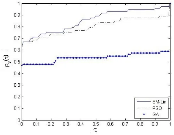
EM-CQ vs. other methods . . . 135 Figure 7.7 Performance profile of the minimum objective function values:

EM-CQ vs. other methods . . . 136 Figure 7.8 Performance profile of the maximum objective function values:

EM-CQ vs. other methods . . . 137 Figure 7.9 Bands of 95% confidence intervals for Performance profile of the

(12)

Chapter 1 Introduction

In engineering, economic and scientific studies, quantitative decisions are frequently mod-eled by optimization concepts and tools. A decision maker may want to find the best decision which corresponds to the minimum (or maximum) of an objective function, while it satisfies a given collection of feasibility constraints.

A large number of such models fall in the category of the conventional continuous optimization problems, notably, the linear and convex optimization. However, there exist cases that the objective function and/or the feasible domain are nonconvex. Then the associated decision model may have many local optimal solutions. The number of such local solutions is not known before solving the problem, and the quality of local and global solutions may vary substantially. These decision models can be very difficult for the conventional optimization methods to become directly applicable. Therefore, innovative global optimization concepts and techniques are needed.

(13)

[44].

1.1 Problem Description

Consider the following global optimization problem with a single objective function:

min f(x) (1.1)

s.t. x∈ S,

where S ={x∈_Rn_|_l_≤_x_≤_{u, g}

j(x)≤0, j = 1, . . . , J}is a nonempty compact subset

of _Rn_{, with the following notations adopted:}

x∈_Rn_{: an} _n _{dimensional real vector of decision variables,}

f ∈_Rn _→_R_{: a real valued continuous objective function,}

l,u∈_Rn_{: explicit lower and upper bounds on} _x,

gj ∈Rn→R, j = 1, . . . , J: a continuous function.

The analytical properties of f being continuous and S being compact guarantee, by the Weierstrass theorem of the classical analysis [101, 44], that the optimal solution set of the global optimization problem is non-empty.

WhenS ={x∈_Rn_{| −∞}_<_x_<_{∞}, the global optimization problem is usually called}

an unconstrained problem. WhenS ={x∈_Rn_|_l_≤_x_≤_{u}, it is called a box constrained}

problem. If S = {x ∈ _Rn_| _Ax _≤ _{b, A} _∈ _Rm×n_, _b _∈ _Rm_{}, it is a linearly constrained}

problem. If S ={x ∈_Rn_| _g

j(x) ≤ 0, gj may be nonlinear function, j = 1, . . . , J}, it is

(14)

In the case of optimizing a single function f, an optimum is either its maximum or minimum, depending on what we are looking for. In global optimization, it is a convention that optimization problems seek their minimizers. Throughout this research we use the minimum objective function value as the optimal value, and the definitions of local and global minima (optima) are listed below.

Global Minimum A global minimum solution of an objective function f : S → _R is an element x∗ ∈ S such that

f(x∗)≤f(x), ∀x∈ S. (1.2)

Neighborhood Let k · k denote the Euclidean norm in _Rn and ε > 0 be a real number, then an ε-neighborhood of a given point y∈_Rn _{is defined as}

N(y, ε)_,{x∈_Rn_{| kx}₋_yk_{< ε}.} _(1.3)

Local Minimum A local minimum solution of an objective function f : S → _R is an element xloc ∈ S with f(xloc)≤f(x) for all xin a neighborhood of xloc, i.e.

∃ ε >0 such that f(xloc)≤f(x), ∀x∈ S ∩N(xloc, ε). (1.4)

Optimal Solution Set The optimal solution set S∗ _{is a subset of} _S _{that contains}

(15)

1.2 Importance of Global Optimization

One of the fundamental principles of our world is the search for an optimal state. Hence global optimization models can be found for numerous real world applications.

It begins in the microworld where atoms in Physics try to form bonds in order to minimize the energy of their electrons [82]. Moreover, when molecules form solid bod-ies during the process of freezing, they try to assume energy-optimal crystal structures. There exist many other processes driven by the laws of Physics that are of global opti-mization nature.

As long as life goes on, we strive for perfection in many areas. We may want to reach a maximum degree of satisfaction with the least amount of effort. In our economy, profits and sales are often maximized and costs are often minimized. Therefore, optimization is one of the oldest sciences governing our daily lives [77].

Another example is the long term financial planning problem described in [63], which is posed as a stochastic program with decision rule. The decision rule requires the pur-chase or sale of assets in each time stage so as to keep constant asset proportions in the portfolio composition. We seek the maximum profit while the decision rule is satisfied, such requirement leads us to a constrained nonconvex optimization problem.

(16)

In Chemical Engineering, the study of molecular conformations is a fascinating sub-ject and molecular mechanics is a widely used method that provides a priori accurate representations of structures and energies for molecules. The small molecules are built with the lowest potential energy. Global minimum potential energy conformations of small molecules are found by utilizing a branch and bound method in [64].

Global optimization works in scheduling problems, too. The problem is to match tasks (or people) and slots (time intervals, machines, rooms, etc.) such that every task is handled in exactly one slot with additional constraints being satisfied. If there are several feasible matchings, one that minimizes some cost or dissatisfaction measure is sought out. Simple scheduling problems such as the linear assignment problem can be formulated as linear programs and solved very efficiently, but the related quadratic assignment problem is one of the hard global optimization problems, where instances with about 30 variables are at the present limit of tractability [3].

There are many other useful applications of global optimization such as the safety verification problem, where a suboptimal local solution could falsely indicate that all safety specifications are met, leading to disastrous consequences if, in actuality, a global solution exists which provides a counterexample that violates some safety specification [57]. For many problems in Chemistry, usually only the global minimizers (of the total energy) correspond to the situations that match reality. The maximum clique problem asks for the maximal number of mutually adjacent vertices in a given graph. (For imple-mentations in robotics, see [78].) More applications can be found in the books of Pint´er [84], and Floudas and Pardalos [29].

(17)

• Linear programming: f is a linear function, and S is a convex set defined by a system of linear equations and inequalities.

• Quadratic programming: f is a quadratic function andS consists of functions that are linear or quadratic.

• D.C. programming: f can be represented as the difference of two convex functions and S consists of equations and inequalities that can be represented as difference of two convex functions.

• Multiplicative programming: f is the product of several convex functions and S consists of equations or inequalities that are represented by convex functions or functions that are product of convex functions.

• Fractional programming: f is the ratio of two real functions and S is convex.

• Concave minimization: f is a concave function and S is a convex set.

• Lipschitz optimization: f is a Lipschitz-continuous function and S consists of in-equalities that are represented by Lipschitz continuous functions.

• Nonlinear programming: Usually f belongs to the class of twice continuously dif-ferentiable functions and S is a nonconvex set.

• Combinatorial optimization: Problems (partially) contain discrete decision vari-ables inf and inS.

(18)

Note that the problem classes listed above are not necessarily distinct. In fact, several of them are contained by more general problem types. For detailed descriptions of most of these model types and their connections, consult the book by Pardalos and Romeijn [81] and the references therein.

1.3 Difficulties in Solving Global Optimization

Prob-lems

Global optimization problems are difficult to solve for two main reasons: the difficulty of finding solutions that satisfy the constraints, and the difficulty of locating real global optimal solutions among local optima.

For the unconstrained problems and box constrained problems, finding a feasible solution does not need too much work. However, when S becomes more complicated — for example, disconnected or highly nonconvex, it becomes quite challenging to obtain a feasible solution. Actually, in many problems such as linear programming problems, determining a feasible solution needs the same amount of effort as getting an optimal solution. Furthermore, the existence of constraints affects the way of searching for an optimal solution. If a method is to keep feasibility throughout the search, it has to follow certain rules restricted by the constraints. If the method violates feasibility in the searching procedure, it has to force the solutions back to the feasible region before it stops in order to produce at least a meaningful solution.

(19)

solved. It is highly possible that a conventional gradient-based method, e.g., Newton’s method, Quasi-Newton method [32, 27], modified steepest descent method [4] or con-jugate gradient method [27] may be trapped by local optima when the feasible region around the global optimum is not well-conditioned [10]. This is because all standard tools of nonlinear optimization such as the derivatives, gradients and subgradients, can at most determine local minima. They cannot tell the differences between local and global solutions.

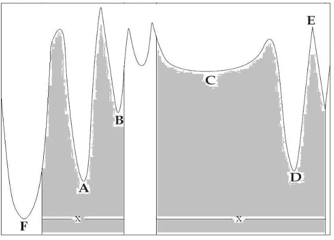
To further illustrate some of the difficulties for a multimodal nonlinear function, we took the example from Birbil [11] and modified it to illustrate our points. Note that the shaded area in Figure 1.1 is the feasible region of the variable x.

(20)

• The global minimizer A is in a deep valley and it is surrounded by tall hills that are difficult to overcome by the gradient-based methods.

• Point B is a promising local minimizer that is in the neighborhood of the global minimizer. A search method may be trapped in B before reaching A.

• The feasible region is disconnected, which means a solution may not be able to improve by going directly fromC toB.

• A search method may spend excessive iterations before passing the shallow basin aroundC.

• The promising local minimizer D may mislead the search method to the regions that are far from the global minimizerA.

• The function is non-differentiable atE, hence the classical gradient-based methods can not be applied.

• The value at point F is smaller than that at A, but the constraints of x indicate that F is an infeasible solution so that it should be eliminated.

(21)

1.4 Contribution of this Research

Birbil and Fang [11, 12] have developed a novel stochastic global optimization method called Electromagnetism-like method (EM) for solving the global optimization problems with bounded (box) constraints. The details of the original method will be shown in the next chapter. In this dissertation, we have further enhanced the EM method for solving linearly and convex quadratically constrained optimization problems (Lin and EM-CQ). We have also tested the methods on some selected problems and implemented EM-Lin for solving a financial planning problem in the real world.

To be more specific, EM-Lin and EM-CQ have been developed with the following properties:

• The proposed methods do not require the derivative information of the objective function, they require function evaluations only.

• To start the algorithms, a number of feasible starting points are needed. EM-Lin and EM-CQ utilize some modified initialization processes to generate starting feasible points.

• We have modified the whole procedure of the original EM method while keeping its essential structure to make the new approaches more competitive in performance.

• The algorithms are designed in the way that, throughout the searching procedures, all the points visited in the search are feasible. Therefore, when the algorithms stop, they can at least provide some meaningful solutions. This also allows us to restart the algorithms directly.

(22)

methods. The result shows that EM-Lin is highly competitive and easy to imple-ment.

• We have compared the proposed methods with other known global optimization methods in a relatively large set of test problems. Our results are more promising than those reported before.

• The general structures of the proposed methods are suitable for the development of parallel computation.

1.5 Outline of the Dissertation

This dissertation is organized as follows: Chapter 2 includes two parts. The first part is a literature review of different global optimization methods, with their advantages and disadvantages. Followed by is a review of the original EM method. The second part is a survey of constrained optimization, which also provides the optimality conditions for solving constrained optimization problems.

(23)

Chapter 2 Literature Review

In this chapter we intend to provide a survey of various global optimization techniques and a review of constrained optimization methods. We will also give an introduction to the EM method for solving problems with bounded constraints.

2.1 Global Optimization Methods

This section provides a classification of global optimization methods.

2.1.1 Taxonomy of Global Optimization Methods

(24)

However, if the dimensionality of the search space becomes higher and/or the objective function of the model becomes more complicated, it is harder to solve the problem in a deterministic manner. It would possibly result in an exhaustive enumeration of the search space, which makes it inapplicable. Thus, for a higher dimensional problem without any special structure, it is perhaps more practical to apply stochastic methods and intelligent heuristic approaches. In general, such methods do not have a complete convergence proof. However, in many cases, they may offer practical tools to handle problems that are out of the reach of theoretically correct, rigorous methodologies.

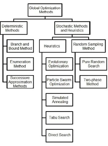
Figure 2.1 gives a taxonomy for global optimization methods which we will present in our review. The review consists of two parts: the first part presents the deterministic global optimization methods. The second part gives a study of stochastic methods and heuristics. In our discussion, some specific approaches are explained in details in the cited literature.

Deterministic Algorithms

This section surveys some deterministic global optimization algorithms. An algorithm is deterministic if it always yields the same results (outputs) when given the same inputs. The focus of this survey is on the general techniques that are applicable to a wide variety of combinatorial and continuous optimization problems that could arise in the real world.

(25)

(26)

the value of a known feasible solution are excluded for further consideration. The parti-tioning continues until a feasible solution is found such that its objective function value is no greater than the lower bound for any subset. Note that as the partitioning goes fur-ther, the number of subproblems may grow exponentially. Therefore it becomes crucial to eliminate the subsets that contain fruitless candidates to reduce the computational burden.

The method was proposed by Land and Doig in 1960 for solving mixed integer pro-gramming problems [56]. The global convergence result of this method is given in [110]. Recently it has been modified and successfully implemented for continuous global opti-mizations. For example, Maranas and Floudas utilized it to find the global minimum potential energy conformations in [64], Maranas et al. applied the method to solve long-term financial planning problems in [63]. For other applications of the branch and bound method, consult, e.g., [85, 76, 39, 44, 51, 84, 28, 100].

Enumeration Method This method is based upon a complete enumeration of all possible solutions. It is applicable for combinatorial optimization problems and some well-structured global optimization models involving concave programming. The disadvantage is that most of such algorithms are computationally intractable for large size problems. For more applications, refer to [44].

Successive Approximation (Relaxation) Method In this approach, the initial optimization problem is replaced by a sequence of relaxed subproblems that are easier to solve. Successive refinement of the subproblems is done by, for example, cutting planes. This approach is applicable for many global optimization problems [44].

(27)

by generally cutting off the feasible regions that do not contain the optimal solutions for sure. Such procedures are popularly used to find integer solutions to mixed integer programming problems, as well as to solving general convex optimization problems. The usage of cutting planes for solving mixed integer programming problems was introduced by Ralph E. Gomory. For continuous optimization problems, it has also been shown that the cutting plane method is useful for concave minimization [9] and convex programming problems [104, 102].

Stochastic Methods

Stochastic methods usually are based on some random sampling of the feasible region. The pure random search method is introduced first. Then, the sample clustering, deter-ministic refinement, and statistical stopping rules can be added as enhancements to the basic scheme of pure random search. Such methods are applicable to both discrete and continuous global optimization problems under very general assumptions.

(28)

convergence speed is slow in this case.

Two-phase Method Many stochastic methods for global optimization consist of two phases: the global phase and local phase. In the global phase, just like the pure ran-dom search method, sample points are drawn from the ran-domain S according to certain distributions with their objective function values calculated. In the local phase, a local optimization method is applied to the set of drawn sample points. The goal of the global phase is to obtain an approximate global extreme while the local phase is to find more precise local extrema. For more details, refer [87]. A number of known methods, such as the Newton’s method and steepest descent method, can be utilized in the local phase.

The pure random search method can be viewed as a simplified two phase method. There are other methods such as the single-start method, multi-start method and clus-tering method [88, 94]. A modification of the pure random search that involves a local method starting from the best point is called a single-start method. A modification that consists of starting local methods from multiple sample points is called a multi-start method.

(29)

Heuristics

Heuristic methods are experience-based techniques that are helpful for problem solving, learning and discovery, especially when the problem is complicated and solving it optimal-ly requires too much effort. Some of these methods are inspired by careful observations of natural phenomena while some are developed merely by intuitive and practical ideas. Usually, a heuristic method produces a good solution (not necessarily optimal) or solves a simpler problem that are closely related to the given complex problem. Heuristics are used to solve some particular problems without validating its true optimality to save computational efforts.

To make heuristics work efficiently, some clever enhancements exploiting expert knowl-edge about the problems at hand are essential. Theoretical work on analyzing the effec-tiveness of useful enhancements is often lacking.

Evolutionary Algorithms Schools of Evolutionary Algorithms have evolved in the past 40 years including the genetic algorithms, developed by Holland [41], evolutionary strategies, developed by Rechenberg [86] and Schwefel [95], and evolutionary program-ming [30]. Each of them constitutes a different approach, however, they are inspired by the same principles of natural evolution.

(30)

Therefore, the efficiency of a genetic algorithm depends on the proper selection of these rules. The tuning of a genetic algorithm requires a considerable amount of insights into the nature of the problem.

Although they are powerful for solving difficult optimization problems [93], a serious handicap of evolutionary algorithms is the heavy computational effort required by large scale problems. In addition, the structure of the encoding used in these algorithms has to be adequately designed for solving the continuous global optimization problems. For more details, please refer [68].

Particle Swarm Optimization Particle Swarm Optimization (PSO) is a population-based stochastic optimization technique developed by Eberhart and Kennedy in 1995 [26], inspired by the social behavior of bird flocking and fish schooling. In PSO, the po-tential solutions, called particles, fly through the problem space by following the current optimum particles. Each particle keeps track of its coordinates corresponding to the best solution it has achieved so far. Its objective function value is also stored aspbest. Another best value that is tracked by the particle swarm optimizer is the best value obtained so far by any particle in the neighborhood. This location is called lbest. When a particle takes all the population as its neighbors, the best value is a global best and is denoted bygbest_{. At each step, a particle in the population changes its velocity toward the} _pbest

and lbest _(or _gbest_{). The velocity is weighted by a random term.}

(31)

Simulated Annealing Simulated Annealing (SA) is a technique based upon the phys-ical analogy of cooling crystal structures that naturally arrive at a stable configuration [52]. The goal of the procedure is to minimize the objective function which represents the potential energy E. In this method, a given state with energy E1 is compared to a

state (with energy E2) that is obtained by moving the particle to another location by

a small displacement. If E1 ≥ E2, the new state is accepted; while if E1 < E2, the

new state is still accepted with a probability of exp(−(E2 −E1)/(kT)), where k is the

Boltzmann constant and T is the temperature of the heat bath. In this way SA can escape the entrapment at local optima. Repeating the process for a large enough number of iterations, the method is proved to be convergent with probability one [20].

The method is originally designed to solve combinatorial minimization problems in [52] and used for continuous problems in [107, 20]. Like evolutionary algorithms, the simulated annealing method is easy to understand and implement. However, in its orig-inal form, the simulated annealing method is convergent but exceedingly slow. Various enhancements of SA make it much faster. Except for simple problems, successful imple-mentation of SA depends very much on the details of adjustments.

Tabu Search The essential idea of this heuristic is to forbid moving to points already visited in the search space, at least within the next few steps. The tabu search method-ology has been primarily used for solving combinatorial optimization problems, but it can be extended to handle continuous global optimizations.

(32)

Direct Search Direct Search methods have been known since at least the 1950s. Clas-sical direct search methods include the Hooke and Jeeves method [43], Nelder-Mead simplex algorithm [75] and Dennis and Torczon’s parallel pattern search algorithm [21]. In a direct search method, if a direction that leads us to a new solution with smaller objective function value, we enlarge the step length in hope of extending the improve-ment. On the other hand, if a new direction leads to a worse position (in terms of the function value), either that direction is not used, or the step length is shrunk. Based on the above concept, each method utilizes different strategy. For example, in Nelder-Mead simplex algorithm, under different conditions, there are procedures of reflection, expan-sion, contraction and reduction [75]. The method finds a minimal solution of a problem by repeatedly performing the above procedures.

2.1.2 General Scheme of the EM Method

Since this research proposes a solution method based on the EM method, it is important to examine carefully the original approach. The approach was proposed by Birbil and Fang [12, 13] and modified by Debels et al [19]. The original EM method works for the nonlinear optimization problems with bounded variables in the following form:

min f(x) s.t. x∈ S,

(2.1)

where f :_Rn→_R is the objective function and

S ={x∈_Rn_{| − ∞}_{< l}

k ≤xk ≤uk <∞, k = 1,2, . . . , n}. (2.2)

(33)

For the above problem, the following parameters are given: the dimension of the problem (n), the real valued function (f(x)) and the lower and upper bounds (lk, uk

for k = 1,2, . . . , n). Since EM works on a set of sample points (population), there is an additional predetermined parameter, r, which denotes the number of points in the population.

The general scheme of the method is given in Algorithm 1. In this scheme an iteration of the algorithm corresponds to one pass of the while loop. There are four procedures: Initialize, Local, CalcF, and Move. The first procedure, Initialize, is used to generate

a population in the feasible region and calculate their initial objective function values. Local is a neighborhood search procedure, which can be applied to one or many points for local refinement at each iteration. CalcF is a procedure to find the moving direction for each solution in the population. Move is a procedure to actually place each solution to a new point in the feasible region.

We use the notation, xi ∈ _Rn_{, to specify the} _ith _{point (solution) of the population.}

Among these points at the current iteration, there is a particular one that has the best objective function value. This point is called the current best point and denoted byxbest_.

Initialization

(34)

Algorithm 1EM for Box-constrained Problems r: number of sample points.

M axiter: maximum number of iterations.

Lsiter: maximum number of local search iterations. δ: local search parameter, δ∈[0,1].

1: Initialize(r)

2: iteration = 1.

3: while iteration < M axiter do

4: Local(δ, Lsiter)

5: CalcF()

6: Move()

7: iteration = iteration + 1.

8: end while

9: Outputxbest and f(xbest).

Algorithm 2Initialize(r)

1: for i= 1 to r do 2: for k= 1 to n do

3: λk ∼U(0,1).

4: xi_k =ll+λk(uk−lk).

5: end for

6: Evaluate f(xi).

7: end for

8: xbest _{= argmin{f(x}i_{), i} _{= 1,}_{2, . . . , r}. (Break the tie with the smallest indexed}

(35)

Local Search

The procedure Local is used to gather the local information at a point xi_{. There are}

many methods that can be used to accomplish this task. In the original method, a very simple one is applied so that we can focus on the EM algorithm itself.

The procedure iterates as follows: firstly, calculate the maximum feasible step length at xi_{. Secondly, locate some feasible neighbors of} _xi _{in different directions. Calculate}

the objective function values of these neighbors and replace xi _{by the one with the}

lowest function value as an improved solution. This procedure repeats until the iteration counter has reached a limit. The parameters, Lsiter and δ which are passed to this procedure, represent the number of iterations and the multiplier for the neighborhood search, respectively.

This algorithm can be applied at every point in the population or only on the current best point xbest_{. In this research we limit the usage of} _Local _{only at} _xbest_.

Calculation of Total Force Vector

The computation of the total force vector is inspired by the superposition principle of electromagnetism theory [18]. In each iteration, a chargeqi of each point xi is calculated

according to f(xi) in (2.3). The charge reflects the efficiency of the objective function value of the corresponding point in the population. The point with a higher charge has a lower function value and tends to attract other points to come closer to it, while the one with lower charge repulses other particles. The charge of particles are defined as

qi = exp

−n× f(x

i₎₋_f(xbest₎

Pr

k=1[f(xk)−f(xbest)]

. (2.3)

(36)

Algorithm 3Local(Lsiter, δ)

Lsiter: the number of maximum iterations in the local search. δ: the multiplier of the step length.

1: iteration = 1.

2: Step lengthα=δmaxk{uk−lk}, k= 1,2, . . . , n.

3: for i= 1 to r do

4: for k= 1 to n do

5: λ1 ∼U(0,1).

6: while iteration < Lsiter do

7: y=xi_.

8: λ2 =U(0,1). 9: if λ1 >0.5then

10: yk= min{yk+λ2α, uk}.

11: else

12: yk= max{yk−λ2α, lk}

13: end if

14: if f(y)< f(xi₎ _then

15: xi =y.

16: iteration = Lsiter - 1.

17: end if

18: iteration = iteration + 1.

19: end while

20: end for

21: end for

(37)

individual component forces,fij_{, between pairs of points}_xi _and_xj_,_j _{= 1,}_{2, . . . , r, j}₆₌_i.

The magnitude of this component force is inversely proportional to the Euclidean distance between the points and directly proportional to the product of their charges.

fi =

r

X

j6=i

fij, i= 1,2, . . . , r, (2.4)

where

fij =   

 

(xj₋_xi₎ qiqj

kxj₋_xi_k2, if f(xj)< f(xi)

(xi₋_xj₎ qiqj

kxj₋_xi_k2, if f(xj)≥f(xi)

, i= 1,2, . . . , r. (2.5)

Closely examining the algorithm, we see that the determination of a direction via the total force vector is similar to the statistical estimation of the gradient vector of f. But the Euclidean distance between two points also affects the magnitude of the force. Therefore, the points that become close enough may lead each other to a direction other than the statistically estimated gradient off.

To avoid being trapped, a modification is performed by adding a perturbed point xp which is the farthest point from the current best point xbest defined by,

xp = argmax{kxbest₋_xi_{k, i}_{= 1,}_{2, . . . , r}.} _(2.6)

At xp, the component forces are perturbed by a random number λ∼U(0,1),

fpj =   

 

(xj₋_xp₎ λqpqj

kxj₋_xp_k2, if f(xj)< f(xp),

(xp₋_xj₎ λqpqj

kxj₋_xp_k2, if f(xj)≥f(xp).

(2.7)

(38)

there exists one point in the population for which the direction of movement may be reversed. The purpose of introducing the perturbed point is to allow the algorithm explore more areas in the feasible region for global convergence.

Algorithm 4CalcF(ν) (ν ∼U(0,1)) ν: the parameter for the perturbed point.

1: xp _{= argmax{kx}best₋_xi_{k, i}_{= 1,}_{2, . . . , r}.}

2: for i= 1 to r do

3: qi = exp

−n× Prf(xi)−f(xbest) k=1[f(xk)−f(xbest)]

.

4: fi ₌_0.

5: end for

6: for i= 1 to r do

7: for j = 1 to r do

8: if i6=j then

9: if i6=pthen

10: fij _{= (x}j ₋_xi₎ qiqj

kxj₋_xi_k2.

11: else

12: λ∼U(0,1).

13: fij _{= (x}j ₋_xi₎ λqiqj

kxj₋_xi_k2. 14: if λ < ν then

15: fij ₌_−fij _{(reverse direction).}

16: end if

17: end if

18: if f(xj₎_{< f}_(xi₎ _then

19: fi ₌_fi₊_fij _{(attraction).}

20: else

21: fi ₌_fi₋_fij _(repulsion).

22: end if

23: end if

24: end for

25: end for

(39)

Movement According to Total Force Vector

After evaluating the total force vector fi_{, the point} _xi _{moves along the direction of the}

force by a random step length λ that is uniformly distributed between 0 and 1, i.e.,

xi_new=xi+λ f

i

kfi_k◦RNG, i= 1,2, . . . , r, i6=best, (2.8)

where xi

new is the updated point and RNG ∈ Rn. In (2.8), f

i

kfi_k ◦RNG is the

one-to-one matching multiplication between _kf_fii_k and RNG. If f

i

j, the jth component of fi, is

nonnegative,RN Gj represents the distance between thejth component ofxi and thejth

component of the upper bound. If fi

j < 0, RN Gj represents the distance between the

jth _{component of} _xi _{and the} _jth _{component of the lower bound. The details are shown}

in the algorithm 5. Note that the best pointxbest _{is not moved.}

Algorithm 5Move(f)

F ={f1_,_f2_{, . . . ,}_fr_{}: the set of total force vectors exerted on} _xi_{, i}_{= 1,}_{2, . . . , r.}

1: for i= 1 to r do

2: if i6=best then

3: λ∼U(0,1).

4: fi ₌ fi

kfi_k.

5: for k = 1 to n do

6: if f_ki >0 then

7: xi

k =xik+λfki(uk−xik).

8: else

9: xi_k =xi_k+λf_ki(xi_k−lk).

10: end if

11: end for

12: end if

13: end for

(40)

Termination Criteria

In the original EM method the procedure is terminated by using a predetermined max-imum number of iterations. According to the test results, in general, 25 iterations per dimension (i.e., M axiter = 25n where n is the dimension of the problem) is satisfactory for converging to the optimum point for those moderate difficulty functions.

Another termination criterion that might be used is the successive number of itera-tions spent without changing the current best point. In other words, if the current best point remains for a certain number of iterations, the algorithm may be stopped. In our new algorithm (EM-Lin), this criterion will be applied. Several other stopping conditions are studied in [103]. One of the frequently used criteria for testing algorithms is to termi-nate the algorithm when the observed objective function value is ε-close to the optimal value [45]. However, this criterion is not appropriate if the global optimum is not known in advance.

2.2 Constrained Optimization Methods

Constrained optimization has an objective function with some explicit constraints to be satisfied. Constraints can be either in the form of equations or inequalities.

A general nonlinear programming problem is in the following form:

min f(x)

s.t. hi(x) = 0, i= 1,2, . . . , m (2.9)

gj(x)≤0, j = 1,2, . . . , p

(41)

where m ≤n and the function f, hi and gi are of real values. We introduce the

vector-valued function h = (h1, h2, . . . , hm) and g = (g1, g2, . . . , gp) and rewrite the problem

as

min f(x)

s.t. h(x) =0 (2.10)

g(x)≤0 x∈_Rn_.

Strict convexity of the objective function f is not sufficient to guarantee a unique minimum. In addition, the feasible domain should be convex to guarantee that the problem has a unique solution.

Because of the constraints, the stationary points of f(x) alone may not be feasible. In fact, the optimal solutions to the constrained problems are often not stationary points of the objective functions. Consequently, the technique of searching for all stationary points of the objective function that also satisfy the constraints does not work. Thus, the necessary conditions for local minimizers are developed in order to reduce the set of possible solutions, and some methods based on the necessary conditions are proposed.

(42)

2.2.1 Constrained Minimization Conditions

Consider the problem with equality constraints

min f(x)

s.t. h(x) =0 (2.11)

x∈_Rn_.

The Lagrangian of a constrained optimization problem is defined to be

l(x,λ) = f(x) +λTh(x), (2.12)

where x∈_Rn _and _λ_∈

Rm.

We now define the regular points of equality constraints.

Regular point for equality constraintsLetx∗be a point satisfying the constraints

h(x∗) =0. (2.13)

Then x∗ is said to be a regular point of the constraints (2.13) if the gradient vectors ∇hi(x∗), i= 1, . . . , m, are linearly independent.

The following theorems give the first order and second order necessary conditions for a point to be a local minimal point subject to equality constraints.

(43)

point. Then there is a λ∈_Rm _{such that,}

∇f(x∗) +λT∇h(x∗) = 0, (2.14) or equivalently,

∇xl(x,λ) = 0, (2.15)

∇λl(x,λ) = 0. (2.16)

Furthermore, the matrix

L(x∗) = F(x∗) +λTH(x∗) (2.17) is positive semi-definite on the tangent plane

M1 ={ y∈Rn | ∇h(x∗)y= 0}, (2.18)

where F and H are the Hessians of f and h, respectively. Now consider the problem with inequality constraints

min f(x)

s.t. h(x) =0 (2.19)

g(x)≤0 x∈_Rn_,

(44)

Here we define a regular point for inequality constraints.

Regular point for inequality constraints Let x∗ be a point satisfying the con-straints

h(x∗) =0, g(x∗)≤0. (2.20)

Let J be the set of indices j for which gj(x∗) = 0, j = 1, . . . , p. Then x∗ is said to be

a regular point of the constraints (2.20) if the gradient vectors ∇hi(x∗), 1≤i≤m and

∇gj(x∗), j ∈ J are linearly independent.

Lemma 2 (Karush-Kuhn-Tucker (KKT) conditions) [62] Let x∗ be a relative minimum point for problem (2.19). Suppose x∗ is a regular point. Then there exist vectors λ∈_Rm _and _µ_∈_Rp _with _µ_≥_{0, such that}

∇f(x∗) +λT∇h(x∗) +µT∇g(x∗) = 0, (2.21)

µT∇g(x∗) =0. (2.22)

Lemma 3 (Second order necessary conditions) [62] Suppose that f, h, g ∈C2 and x∗ is a regular point. If x∗ is a relative minimum point of the problem (2.19), then there exist λ ∈ _Rm _and _µ _∈ _Rp _with _µ _≥ _{0, such that (2.21) and (2.22) hold and the}

Hessian matrix

L(x∗) = F(x∗) +λTH(x∗) +µTG(x∗), (2.23) is positive semi-definite on the subspace

(45)

where F,H and G are the Hessians off, h and g, respectively, and

J ={ j | gj(x∗) = 0, µj >0, j = 1, . . . , p}. (2.25)

After introducing the necessary conditions for local minimum solutions, we are going to bring in some practical methods for solving the constrained optimization problems. Some of these methods are designed based on the necessary conditions.

2.2.2 Primal Methods

A primal method directly works on the original problem by searching through the fea-sible region for an optimal solution. Each candidate in the process is feafea-sible and the value of the objective function usually decreases iteration by iteration. There are several advantages of the primal methods. First, if the process terminates before reaching the solution, the terminating point is still feasible. The other advantage is that most primal methods are more applicable for general nonlinear programming problems. However, the primal methods can lead to some difficulties caused by the feasible domain, and they may lack the global convergence proof.

Some commonly seen primal methods include the feasible direction method, active set method and gradient projection method.

Feasible Direction Method

The idea of feasible direction method is to take steps through the feasible region of the form

(46)

wheredi _∈_Rn_{is a direction vector and}_α

i is a nonnegative scalar used as the step length.

A feasible direction method can be considered as a natural extension of the unconstrained descent method. Each step is the composition of selecting a feasible direction di _{and a}

constrained line search for an appropriate step lengthαi >0. The algorithm is originally

proposed by Zoutendijk [115] and has been modified over the last few decades. For more information, please refer [62, 54].

Active Set Method

Problems with inequality constraints can be approached with an active set method. The idea of the active set method is to partition the inequality constraints into two groups: those are active and those are inactive. The inactive constraints are ignored since the points can move in its neighborhood without violating the inactive constraints. A working set is defined as the index set of active constraints. By dynamically adding and dropping constraints from the working set, the correct set of active constraints is determined in the search process. Convergence cannot be guaranteed for many of this approach because the working set may change all the time. But in practice the active set method with various refinements are often very effective. Details the of active set method are described in [62, 79, 73].

Gradient Projection Method

(47)

implementation-s, and found to be effective in solving general nonlinear programming problems. The method is proposed by Rosen in [90] to solve nonlinear programming problems with lin-ear constraints. Later it is generalized to solve nonlinlin-ear programming problems with nonlinear constraints in [91].

2.2.3 Dual Methods

Dual methods are based on the fact that the solution point of a constrained problem is determined by the Lagrangian multipliers which are the unknowns associated with the problem. Therefore, instead of solving the primal problem, a dual method tries to find the Lagrangian multipliers for the dual problem.

Lemma 4 (Local duality theorem for equality constraints) [62] Suppose that the problem

min f(x) (2.27)

s.t. h(x) =0

x∈_Rn, h(x)∈_Rm,

has a local minimum x∗ with the corresponding Lagrangian vector λ∗ ∈ _Rm_{. Suppose}

thatx∗ is a regular point and the corresponding Hessian matrixL(x∗) in (2.17) is positive definite. Define the dual function

φ(λ) = min

x {f(x) +λ

T_h(x)}, _λ_∈

(48)

where the minimum is taken locally in the neighborhood of x∗. Then the dual problem

max φ(λ) (2.29)

has a local solution at λ∗ with x∗ being the solution of (2.28) forφ(λ∗).

Lemma 5 (Local duality theorem for inequality constraints) [62] Suppose that the problem

min f(x)

s.t. h(x) = 0 (2.30)

g(x)≤0

x∈_Rn_, _h(x)_∈

Rm, g(x)∈_Rp_,

has a local minimum x∗ with the corresponding Lagrangian vectors λ∗ ∈ _Rm _and _µ∗ _∈

Rp_, _µ∗ _≥ _{0. Suppose that} _x∗ _{is a regular point and the corresponding Hessian matrix}

L(x∗) in (2.23) is positive definite. Define the dual function φ(λ,µ) = min

x {f(x) +λ

T

h(x) +µTg(x)}, λ∈_Rm, µ∈_Rp, (2.31)

where the minimum is taken locally in the neighborhood of x∗. Then the dual problem

max φ(λ,µ) (2.32)

achieves a local solution at λ∗ and µ∗ ≥ 0 with x∗ being the solution of (2.31) for φ(λ∗,µ∗).

(49)

mul-tipliers λ and µ. Therefore, when we find the local maximizer of the dual problem, the solution to the original problemx∗ can be obtained. Details of the dual methods are pre-sented in [62]. In [36, 58, 105], the dual methods have been proposed to solve quadratic programming problems.

2.2.4 Penalty and Barrier Function Methods

Penalty and barrier function methods are similar methods that utilize different forms of cost functions which are added to the original objective functions.

Penalty Method Penalty method approximates a constrained problem by an uncon-strained one by assigning a high cost to points that are not feasible. As the approx-imation is made more exact (by adjusting the penalty parameter), the solution of the unconstrained penalty problem approaches the solution of the original problem. In other words, a penalty method may use a sequence of exterior methods and the feasibility is obtained only at the optimum.

The advantage of the penalty method is that it is less likely to be stuck in a feasible pocket with a local minimum. Furthermore, the penalty method is more robust because in practice one may often have an infeasible starting point. However, penalty functions typically require more function evaluations. Details of the penalty method are described in [62, 98].

(50)

approaches the solution of the original constrained problem from the interior of the fea-sible region. So the barrier method is characterized by its ability of preserving feasibility at all times. This is the advantage of the barrier method because even if it does not converge, one will still have a feasible solution. Details of the barrier method can be found in [14, 62].

(51)

Chapter 3 Electromagnetism-like Method for

Linearly Constrained Problems

(EM-Lin)

A novel algorithm called Electromagnetism-like Mechanism (EM) was introduced in [13]. Its general scheme has been introduced in the previous chapter for solving optimization problems with bounded variables. The objective of this research is to adapt the concept of the EM method to develop an algorithm for solving global optimization problems with more general constraints.

(52)

3.1 Outline of EM-Lin

We address the linearly constrained optimization problem in the following form:

min f(x) s.t. Ax≤b

x∈Ω,

(3.1)

where Ω ={x∈ _Rn_| _l_≤ _x_≤_u}, _l,_u _∈

Rn, A ∈_Rm0×n _and _b_∈ _Rm0_{. In this case, the}

feasible region S becomes

S ={x∈_Rn_| _Ax_≤_b, _l_≤_x_≤_u}. _(3.2)

To simplify the formulation, we may combine the box constraints and linear con-straints together. Let

A=                 A .. . −ei .. . ei .. .                

and b=                 b .. . −li .. . ui .. .                

, i= 1,2, . . . , n. (3.3)

where ei _{is a row vector with 1 being its} _ith _{element and 0 otherwise. Then,}

S = {x∈_Rn| Ax≤b} ∩ {x∈_Rn| −eix≤ −li, i= 1,2, . . . , n} (3.4)

∩{x∈_Rn_| _ei_x_≤_u

(53)

Therefore, by comparing the formulas of (3.3) and (3.4), we have

S ={x∈_Rn _| _Ax_≤_b}. _(3.5)

The equivalent form of (3.1) then becomes

min f(x) s.t. Ax≤b.

(3.6)

We assume that A∈_Rm×n _and _b _∈

Rm.

Our goal is to design an algorithm seeking for the global solutions while maintaining the feasibility of the solution in each iteration. In this way, the algorithm always provides a meaningful solution even when it stops prematurely.

EM-Lin contains four major steps: Initialize, Local, CalcF and Move. Comparing with the original EM method, the first step, Initialize, needs to be replaced by a new procedure, since the known one is no longer applicable for the linearly constrained case. A direct search is implemented in theLocal step to achieve a better performance. TheCalcF procedure works well for the new case and we retain it. The original Move procedure may produce points which violate the linear constraints. Therefore, some adjustments are needed. New terminating criteria are also added to make the algorithm more efficient. We describe below in Algorithm 6 the main structure of the revised EM algorithm for solving linearly constrained problems of (3.6).

(54)

Algorithm 6EM for linearly constrained Problem

1: Define Parameters. Set up the initial parameters.

2: ∆tol, ∆: the stopping tolerance and the initial stopping parameter, respectively. 3: φ >1, 0< θ <1: the increasing and the decreasing factor, respectively.

4: r: the initial population size.

5: Initialize. Randomly generate the initial feasible population {x1_,_x2_{, . . . ,}_xr_}.

6: Evaluate the initial active pointf(xi_{), i}_{= 1,}_{2, . . . , r.}

7: xbest ₌_x1_{, f}best ₌_f_(xbest_).

8: Set Successf ul improvement=true.

9: while the stopping criteria are not satisfied do

10: Set xbest _{= argmin{f}_(xi_{), i}_{= 1,}_{2, . . . , r}.}

11: if f(xbest)< fbest then

12: Set fbest ₌_f_(xbest_{), set} _{Successf ul improvement}₌_true. 13: ∆ =φ×∆ (increase the stopping parameter).

14: Skip the Local Search step and go to CalcF(ν).

15: else

16: Apply Local Search at xbest_{, which provides the updated} _xbest _{and updated}

Successf ul improvement.

17: if Successf ul improvement =f alse then

18: ∆ =θ×∆ (decrease the stopping parameter).

19: end if

20: end if

21: CalcF(ν).

22: Move.

23: Check Stopping Criterion. (Check Section 3.6 for details.)

24: end while

(55)

3.2 Initialization

Before starting the main loop of the algorithm, a set of initial points that lie inside the polyhedron

S ={x∈_Rn_| _Ax_≤_b} _(3.7)

need to be generated.

When only simple bounds (that is, l ≤ x ≤ u with l and u being the lower and upper bounds) are present in the problem, an initial feasible population can be randomly generated by using a uniform distribution. However, generating an initial feasible pop-ulation for a linearly constrained problem is not that simple. There are several ways to accomplish the task, and our algorithm considers all of them.

For generating a feasible population satisfying the linear constraints, one strategy would be firstly to ignore the linear constraints and randomly generate points. Then a newly generated point is accepted if it satisfies the constraints. This strategy is

straightforward and easy to implement. However, such a strategy may not be efficient for generating a diverse feasible population. When the polyhedron formed by the linear constraints is relatively small compared to the region formed by the simple bounds, the probability that a randomly generated point falls in the polyhedron would be low. We keep this method of generating the initial feasible population in our algorithm and use it when other methods fail to provide the initial feasible population.

(56)

it-eration, we are able to obtain some feasible solutions to the problem. Finally, the convex combinations of these solutions can be used as the initial feasible points. Since the linear programming problem can be solved in polynomial time by the interior point method, this method may finish generating the initial feasible population in polynomial time.

The third way of providing an initial feasible population is explained below. First, find an interior point x0 that lies inside the feasible domain S. This can be done in several ways, one of which is solving a linear programming problem,

max t

s.t. Ax+te≤b

(3.8)

with the optimal solution (x∗, t∗), where e = (1,1, . . . ,1)T _∈ _Rm_{. If} _t∗ _> _0, _x∗ _can

be accepted as x0. Then, from x0, a set of random vectors {v1_,_v2_{, . . . ,}_vq_} _{pointing to}

different directions are generated. Before extending these vectors to hit the boundary of S, if we choose the step length αi carefully, the points

xi =x0+αivi, αi >0, i= 1,2, . . . , q, (3.9)

(57)

feasible region, the points generated are feasible. Furthermore, the maximum-volume ellipsoid helps us to distribute the points as diverse as possible.

The computation of the maximum-volume ellipsoid inscribed inside the feasible region is carried out by the interior point method developed by Zhang and Gao [113].

In their paper, a polytope P = {x ∈ _Rn _| _Cx _≤ _d} _{is considered as the feasible}

region, where C ∈ _Rp×n_{, p > n, and} _d _∈

Rp. Two assumptions are made throughout the paper,

1. The matrix C has full column rank and contains no zero rows.

2. There exists a strictly interior point ¯x∈ P such that C¯x<d.

To produce C and d which satisfy the assumptions, some preprocesses are needed. Consider the assumption 1 first, if A∈_Rm×n _{in the original feasible region} _S _{meets the}

requirement that m > n and has full column rank, the first assumption is satisfied. A andb in (3.6) can be used asC andd. Ifm ≤n, artificial bounds are added to make the new constraint matrix C have more rows than columns and have the full column rank. Then the calculation of the inscribed ellipsoid is doable. Since the new feasible region is contained in S, the generated points are feasible.

To satisfy the second assumption, we solve a linear programming problem,

max t

s.t. Cx+te≤d,

(3.10)

where e ∈ _Rp _{is a column vector with 1 at all positions. Suppose that the solution of}

(58)

To find a maximum-volume ellipsoid inscribed in P ={x∈_Rn _|_Cx_≤_{d}, one needs}

a centerxc_{and a nonsingular scaling matrix}_E _∈_Rn×n_{. Then an ellipsoid can be defined}

as

ξ(xc, E) = {v∈_Rn _| _v₌_xc₊_Es, _{ksk ≤}_1}, _(3.11)

where k.kis the Euclidean norm in _Rn_.

The volume of the ellipsoid ξ(xc_{, E) is defined to be}

Vol(ξ) =Vndet(E), (3.12)

where Vn is the volume of the n-dimensional unit ball. Then, a convex programming

problem MAX-VOL is constructed as in [113]:

min

x,E −det(E) (3.13)

s.t. cjx+kEcjk ≤dj, j = 1,2, . . . , p

E ∈ Sn

+,

where cj is the jth row of C, dj is the jth element of d and S+n represents the cone of

all symmetric positive definite matrices in_Rn_{. Problem (3.13) is a convex programming}

problem and it has a unique solution (xc∗_{, E}∗₎_∈

Rn_{× S}n

+.

In [113], an interior point method is used to solve the problem. According to the paper, the interior point method is well-defined, the solution is unique and the algorithm is globally convergent. Though it is unlikely that polynomial convergence could be proven for the algorithm, it is fast enough in experiments. Furthermore, the method described in the above paper is easy to incorporate into our algorithm.

(59)

are obtained in the above step, the initial feasible points can be generated withinξ(xc∗_{, E}∗₎

using the following equation:

xi =xc∗+E∗ηi, i= 1,2, . . . , r, (3.14) where ηi _∈ _Rn _and _kηi_{k ≤} _{1, i} _{= 1,}_{2, . . . , r, are vectors generated along different}

coordinates.

In our algorithm, the method of finding the maximum volume ellipsoid is first applied since it may generate diverse initial solutions. If the interior point method is unable to solve the MAX-VOL problem (3.13) in a certain number of iterations, we turn to use the third method which is described previously. When the calculated step lengths in the third method are too small, which means the generated points are too close to x0 in (3.9), the second method is applied. Finally, if the second method still does not provide enough initial feasible solutions, the first method has to be utilized, though it appears to be inefficient.

3.3 Local Search

The procedure Local is used to gather the local information of a pointxi _{and find better}

solutions in the neighborhood of xi_{. As stated in [12, 13], many powerful local search}

(60)

Algorithm 7Initialize(S, r)

S: the feasible region given by the problem. r: size of the initial population.

1: Set N2, N3 and N4 as the thresholds for methods 2,3 and 4, respectively. 2: Apply method 4.

3: if fail to solve MAX-VOL inN4 iterations then

4: Apply method 3. Stop when the # of initial feasible solutions = r.

5: if in method 3 the step length is smaller than N3 then

6: Apply method 2. Stop when the # of initial feasible solutions = r.

7: if the # of recorded feasible solutions is smaller than N2 then 8: Apply method 1. Stop when the # of initial feasible solutions = r.

9: if the # of initial feasible solutions < r then

10: Return error.

11: end if

12: end if

13: end if

14: end if

15: Output the initial feasible solutions {x1_,_x2_{, . . . ,}_xr_}.

the new xbest. If no point is better than the original xbest, the best point remains the same. The structure of the direct search is given as below.

The calculation of the matrix J formed by the set of directions (line 3, Algorithm 8) is a key step. When xbest _{is not close to the boundary of the feasible domain} _{S, the}

problem can be considered as an unconstrained one. In this case J _, [j1_,_j2_{, . . . ,}_jk_{] =}_I,

the identity matrix, is a good choice. Otherwise, the set of searching directions{j1_{, . . . ,}_jk_}

should reflect the geometry of any portion of the boundary of the feasible region near xbest.

To calculate J in the latter case, we adopt the idea in [53]. Let ai be the ith row of A in (3.3) and bi be the ith element of b in (3.3). For a given >0, define

(61)

Algorithm 8Local Search (xbest_{, k,}_∆)

xbest_{: the current best point.}

k: the number of searching directions. ∆: the stopping parameter.

1: Set φ >1 to be the increasing factor.

2: LetF(x) =

f(x), if x∈ S, +∞, otherwise.

3: Compute the matrixJ formed by the set of directions, J = [j1_{, . . . ,}_jk_].

4: for i= 1 to k do

5: if F(xbest+ ∆×ji)< F(xbest)then

6: Set xbest ₌_xbest_{+ ∆}_×_ji_, _{Successf ul improvement}₌_true.

7: Set ∆ = ∆×φ (increase the stopping parameter).

8: Stop the Local search method and return the new xbest.

9: end if

10: end for

11: if F(xbest+ ∆×ji)≥F(xbest) for allji inJ then

12: Stop the Local search method, set Successf ul improvement= f alse and return the original xbest_.

13: end if

An Electromagnetism-like Method for Solving Linearly and Quadratically Constrained Optimization Problems.

ABSTRACT

DEDICATION

BIOGRAPHY

ACKNOWLEDGEMENTS

TABLE OF CONTENTS

LIST OF TABLES

LIST OF FIGURES

Chapter 1

Introduction

1.1

Problem Description

1.2

Importance of Global Optimization

1.3

Difficulties in Solving Global Optimization

Prob-lems

1.4

Contribution of this Research

1.5

Outline of the Dissertation

Chapter 2

Literature Review

2.1

Global Optimization Methods

2.1.1

Taxonomy of Global Optimization Methods

2.1.2

General Scheme of the EM Method

2.2

Constrained Optimization Methods

2.2.1

Constrained Minimization Conditions

2.2.2

Primal Methods

2.2.3

Dual Methods

2.2.4

Penalty and Barrier Function Methods

Chapter 3

Electromagnetism-like Method for

Linearly Constrained Problems

(EM-Lin)

3.1

Outline of EM-Lin

3.2

Initialization

3.3

Local Search