University of Windsor University of Windsor
Scholarship at UWindsor
Scholarship at UWindsor
Electronic Theses and Dissertations Theses, Dissertations, and Major Papers
2012
New Detection Algorithms for Single Input Multiple Output
New Detection Algorithms for Single Input Multiple Output
Systems with Carrier Frequency Offset
Systems with Carrier Frequency Offset
Shayondip Sinha University of Windsor
Follow this and additional works at: https://scholar.uwindsor.ca/etd
Recommended Citation Recommended Citation
Sinha, Shayondip, "New Detection Algorithms for Single Input Multiple Output Systems with Carrier Frequency Offset" (2012). Electronic Theses and Dissertations. 142.
https://scholar.uwindsor.ca/etd/142
NEW DETECTION ALGORITHMS FOR SINGLE INPUT MULTIPLE OUTPUT SYSTEMS WITH CARRIER FREQUENCY OFFSET
by
Shayondip Sinha
A Thesis
Submitted to the Faculty of Graduate Studies through Electrical and Computer Engineering in Partial Fulfillment of the Requirements for the Degree of Master of Applied Science at the
University of Windsor
Windsor, Ontario, Canada
2012
New Detection Algorithms For Single Input Multiple Output Systems with Carrier Frequency Offset
by
Shayondip Sinha
APPROVED BY:
Dr. Scott Goodwin School of Computer Science
Dr. Kemal Tepe
Department of Electrical and Computer Engineering
Dr. Behnam Shahrrava
Department of Electrical and Computer Engineering
TBA Chair of Defense
Co-Authorship Declaration
I hereby declare that this thesis incorporates material that is result of joint research,
as follows:
This thesis also incorporates the outcome of a joint research undertaken in
collab-oration with Garima Deep under the supervision of professor Dr. Behnam Shahrrava.
The collaboration is covered in Chapter 4 of the thesis. In all cases, the key ideas,
primary contributions, experimental designs, data analysis and interpretation, were
performed by the author, and the contributions of co-authors were primarily through
the provision of proof reading and reviewing the research papers regarding the
tech-nical content.
I am aware of the University of Windsor Senate Policy on Authorship and I
cer-tify that I have properly acknowledged the contribution of other researchers to my
thesis, and have obtained written permission from each of the co-authors to include
the above materials in my thesis.
I certify that, with the above qualification, this thesis, and the research to which
Declaration of Previous Publications
This thesis includes 2 original papers that have been previously submitted for
publi-cation in peer reviewed journals and conferences, as follows:
Thesis Chapter Publication title/full citation Publication
status
Chapter 4 S. Sinha, B. Shahrrava, G. Deep “A New SIMO
Detector with Unknown Channel and Carrier
Frequency Offset”; IEEE International Global
Telecommunication Conference
submitted
Chapter 4 S. Sinha, B. Shahrrava, G. Deep “A New ML
De-tector for SIMO systems with Imperfect Channel
and Carrier Frequency Offset Estimation”; 2012
IEEE Workshop on Signal Processing Systems
submitted
I certify that I have obtained a written permission from the copyright owner(s)
to include the above published material(s) in my thesis. I certify that the above
material describes work completed during my registration as graduate student at the
University of Windsor.
I declare that, to the best of my knowledge, my thesis does not infringe upon
quotations, or any other material from the work of other people included in my
the-sis, published or otherwise, are fully acknowledged in accordance with the standard
referencing practices. Furthermore, to the extent that I have included copyrighted
material that surpasses the bounds of fair dealing within the meaning of the Canada
Copyright Act, I certify that I have obtained a written permission from the copyright
owner(s) to include such material(s) in my thesis.
I declare that this is a true copy of my thesis, including any final revisions, as
approved by my thesis committee and the Graduate Studies office, and that this thesis
Abstract
The performance of a multiple antenna wireless communication (WC) system depends
significantly on the type of detection algorithm used at the receiver. This thesis
proposes three different types of detection algorithms for single input multiple output
(SIMO) systems and concludes with a comparative study of their performance in
terms of bit error rate (BER). The proposed algorithms are based on the following
classical methods:
• Maximum Likelihood (ML) detection
• Maximal Ratio Combining (MRC) scheme
• Minimum Mean Square Error (MMSE) criterion detection
The major challenge in any practical WC system is the imperfect knowledge of channel
state information (CSI) and carrier frequency offset (CFO) at the receiver. The
novel algorithms proposed in this thesis aim for optimal detection of the transmitted
signal and are derived for a system in the presence of both CSI and CFO estimation
errors. They can be treated as a generalized form of their respective type and it
is mathematically shown that the conventional algorithms are a special case in the
absence of the estimation error. Finally, the performance of the novel algorithms is
demonstrated by exhaustive simulation for multi-level modulation techniques of phase
shift keying (PSK) and quadrature amplitude modulation (QAM) with increasing
to my
mother, father
Acknowledgements
Hard work paves the way to success, but it is also very important to be shown the
right path. I would like to take this opportunity to express by thanks and gratitude
to all, who gave me direction and supported me during my time at the University.
Firstly, I would like to thank my supervisor, Dr. Behnam Shahrrava, for his
guid-ance, support and encouragement. He has been a great mentor and his enthusiastic
involvement in my research was truly motivational. His valuable suggestions have
always helped me academically and also to develop professionally. I would also like
to thank Dr. Scott Goodwin and Dr. Kemal Tepe for their invaluable advice. I am
thankful to Ms. Andria Ballo, Ms. Shelby Marchand and Mr. Frank Cicchello for
providing me with an excellent work environment in the department.
I am highly grateful to all my friends, in particular Dibyendu Mukherjee,
Ashir-bani Saha, Dr. Gaurav Bhatnagar and Garima Deep for their endless assistance,
support and encouragement in the completion of this research.
I dedicate this work to my family and thank them for their love and belief in my
Table of Contents
Page
Co-Authorship Declaration . . . . iii
Declaration of Previous Publications . . . . iv
Abstract . . . . vi
Acknowledgements . . . . viii
List of Figures . . . . xii
List of Acronyms . . . . xiv
Glossary of Symbols . . . . xvi
1 Introduction . . . . 1
1.1 MIMO Systems . . . 3
1.1.1 Types of MIMO Systems . . . 4
1.1.1.1 Multi-antenna MIMO . . . 4
1.1.1.2 Multi-user MIMO . . . 5
1.2 Modulation and Demodulation . . . 6
1.2.1 Phase Shift Keying . . . 8
1.2.2 Quadrature Amplitude Modulation . . . 9
1.3 Motivation and Problem . . . 10
1.3.1 Multi-Channel Fading . . . 10
1.3.1.1 Rayleigh fading model . . . 11
1.3.2 Carrier Frequency Offset . . . 13
1.5 Organization of Thesis . . . 14
2 SIMO Detection Techniques . . . . 16
2.1 Maximum Likelihood Detection . . . 17
2.2 Linear Combiner . . . 19
2.2.1 Maximal Ratio Combiner . . . 20
2.2.2 ML Detector . . . 21
2.3 L-MMSE Detector . . . 22
2.4 Performance Simulation for SIMO . . . 24
3 Effect of Imperfect Estimation . . . . 26
3.1 Imperfect Channel Estimation . . . 26
3.1.1 ML Detector . . . 28
3.1.2 Linear Combiner . . . 29
3.1.3 L-MMSE . . . 30
3.1.4 Performance Simulation . . . 31
3.2 Imperfect CFO Estimation . . . 38
3.2.1 ML Detector . . . 38
3.2.2 Linear Combiner . . . 39
3.2.3 L-MMSE . . . 40
3.2.4 Performance Simulation . . . 41
4 Proposed Detection Algorithms in the presence of CSI and CFO estimation errors . . . . 48
4.1 Previous Work and Assumptions . . . 49
4.2 ML Detector . . . 51
4.2.1 Convergence to Conventional Metric . . . 53
4.3 Linear Combiner . . . 54
4.3.1 Combiner Design Methodology . . . 54
4.3.2 ML Detection Methodology . . . 55
4.4 L-MMSE . . . 56
4.4.1 Convergence to Conventional L-MMSE . . . 58
5 Simulation and Performance Analysis . . . . 60
5.1 Proposed ML Detector . . . 62
5.2 Proposed Linear Combiner . . . 66
5.3 Proposed L-MMSE Detector . . . 70
6 Conclusion and Future Work . . . . 75
References . . . . 77
Appendix A Mathematical Calculations . . . . 87
A.1 Conditional PDF of CAFO . . . 87
A.2 Conditional Expectation of CAFO . . . 89
A.3 Conditional Expectation of Received Signal . . . 90
A.4 Conditional Variance of Received Signal . . . 91
List of Figures
1.1 Block diagram of a communication system. . . 2
1.2 Types of multi-antenna MIMO. . . 4
1.3 Illustration of M-ary PSK/QAM modulation and demodulation . . . 6
1.4 Signal space diagram of PSK modulations. . . 8
1.5 Signal space diagram of QAM modulations. . . 9
1.6 Multipath propagation in a wireless channel . . . 10
2.1 Two branch SIMO . . . 16
2.2 Linear Combiner . . . 19
2.3 Vector diagram of MSE . . . 23
2.4 Performance of two branch SIMO . . . 25
3.1 ML detector with channel estimator . . . 28
3.2 MRC with channel estimator . . . 29
3.3 MMSE detector with channel estimator . . . 30
3.4 Performance of 4-PSK SIMO with channel estimation error . . . 32
3.5 Performance of 8-PSK SIMO with channel estimation error . . . 33
3.6 Performance of 16-PSK SIMO with channel estimation error . . . 34
3.7 Performance of 4-QAM SIMO with channel estimation error . . . 35
3.8 Performance of 16-QAM SIMO with channel estimation error . . . 36
3.9 Performance of 64-QAM SIMO with channel estimation error . . . 37
3.11 MRC with channel and CFO estimator . . . 40
3.12 MMSE detector with channel and CFO estimator . . . 41
3.13 Performance of 4-PSK SIMO with CSI and CFO estimation error . . 42
3.14 Performance of 8-PSK SIMO with CSI and CFO estimation error . . 43
3.15 Performance of 16-PSK SIMO with CSI and CFO estimation error . . 44
3.16 Performance of 4-QAM SIMO with CSI and CFO estimation error . . 45
3.17 Performance of 16-QAM SIMO with CSI and CFO estimation error . 46 3.18 Performance of 64-QAM SIMO with CSI and CFO estimation error . 47 5.1 Proposed ML detector 4-PSK . . . 62
5.2 Proposed ML detector 8-PSK and 16-PSK . . . 63
5.3 Proposed ML detector 4-QAM . . . 64
5.4 Proposed ML detector 16-QAM and 64-QAM . . . 65
5.5 Proposed linear combiner 4-PSK . . . 66
5.6 Proposed linear combiner 8-PSK and 16-PSK . . . 67
5.7 Proposed linear combiner 4-QAM . . . 68
5.8 Proposed linear combiner 16-QAM and 64-QAM . . . 69
5.9 Proposed L-MMSE 4-PSK . . . 70
5.10 Proposed L-MMSE 8-PSK and 16-PSK . . . 71
5.11 Proposed L-MMSE 4-QAM . . . 72
List of Acronyms
ASK Amplitude shift keying
AWGN Additive white Gaussian noise
BER Bit error rate
CAFO Carrier angular frequency offset
CFO Carrier frequency offset
CSI Channel state information
ICI Inter carrier interference
iid Independent identically distributed
LTE Long term evolution
MAP Maximum a posteriori
MIMO Multiple input antenna and multiple output antenna
MISO Multiple input antenna and single output antenna
ML Maximum likelihood
MMSE Minimum mean square error criterion
MSE Mean square error
OFDM Orthogonal frequency division multiplexing
PDF Probability density function
PSK Phase shift keying
QAM Quadrature amplitude modulation
QoS Quality of service
RF Radio frequency
RV Random variable
SIMO Single input antenna and multiple output antenna
SISO Single input antenna and single output antenna
SNR Signal to noise ratio
Glossary of Symbols
[.]T Transpose of a vector or matrix
[.]∗ Complex conjugate of a vector or matrix
[.]H Hermitian of a vector or matrix
∥.∥ Euclidean norm
ℜ{.} Real value of a variable
⊥ Orthogonal
ln Natural logarithm
E[.] Expected value of a random variable
V ar[.] Variance of a random variable
P (x) Probability of the occurrence ofx
j √−1
f(.) Probability density function
A∼ N(µ, σ2
Chapter 1
Introduction
The communication industry is undoubtedly the fastest growing sector of the global
industrial development as it has made its impact on every stratum of the society.
Wireless networks have been a significant contributor since its development from the
pre-Industrial age. Signals in the form of torch beams, smokes etc. were
predom-inantly used as wireless signals which eventually lead to the invention of telegraph
networks in 1838 by Samuel Morse. This later developed into voice communication,
which is prevalent as telephony. Years later in 1895, Marconi performed radio
trans-mission over about 18 miles giving birth to a new genre of WC. Since then, WC has
been a hot topic for research and development all across the world. The challenges
faced by any communication network is broadly categorized by Weaver [1] as three
level problem:
Level A: Technical problem.
How accurately the symbols of communication be transmitted?
Level B: Semantic problem.
How precisely do the transmitted symbol convey the desired meaning?
Level C:Effectiveness problem.
Figure 1.1: Block diagram of a communication system.
Shannon [2] has described these problems with a very basic block diagram of a
communication system model as given in Fig. 1.1. The technical problems broadly deal with, how accurately the given information is transmitted. This problem is
han-dled by the information source and transmitter blocks. The information source block
picks a desired message from a set of possible messages and the transmitter block
converts them into signals which are transmitted over the channel. This process
employs different encoding methodologies, modulation techniques, diversity schemes,
etc. Few of these are broadly discussed in later sections of the thesis. The semantic problems are concerned with, how well the receiver interprets the meaning of the in-formation. The transmitted signal undergoes certain level of distortion, or is added
with extraneous undesired signals called Noise, while in the communication channel.
This deteriorates the quality of the transmission and increases the uncertainty of the
receiver to select the original signal. The receiver here acts as an inverse transmitter
The thesis predominantly concentrates on thesemantic problems of WC networks. The advent of voice telephony, transmission of high quality video and images require
wireless networks to maintain high quality of service (QoS). However, the QoS highly
depreciates due to multi path transmission, fading channels etc. In order to obtain
a higher QoS in such cases, it is important to achieve reliable data transmission and
optimal detection of the data at the receiver. Improvement of 1-dB in signal to noise
ratio (SNR) may reduce BER by 90% for an additive white Gaussian noise (AWGN)
channel. However, for multi path fading channels similar reduction in BER can be
achieved by over 10-dB improvement in SNR.
1.1
MIMO Systems
The performance of a WC system in a multi path fading channel can be significantly
improved by employing diversity technique where multiple copies of the same infor-mation signal is transmitted to the receiver. There are typically five differentdiversity
techniques that are used practically [3, 4]:
1. Frequency diversity - Multiple carriers are used to transmit the same signal.
2. Time diversity - The same signal is periodically transmitted multiple times.
3. Space diversity - Multiple antennas are used to transmit or receive multiple copies of the same signal. This technique is also calledAntennae diversity.
4. Polarization diversity - The variation of the electric and magnetic fields of the signal is used to achieve multiple transmission.
Multiple input multiple output (MIMO), systems are most widely researched and
implemented in WC systems using diversity techniques. MIMO is one of the most optimal approaches for improving reliability of data transmission which does not
require additional spectral resources and instead exploits the spatial diversity provided
by multiple transmit and receive antennas. Reliability in data transmission is attained
when the same data are sent over multiple paths and multiple copies of the data are
received with different antennas. Here, the channel capacity is enhanced as the loss
of data due to fading in one channel can be compensated for, by the other receiver.
1.1.1
Types of MIMO Systems
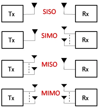
MIMO systems can be broadly categorized into two different types
1.1.1.1 Multi-antenna MIMO
Figure 1.2: Types of multi-antenna MIMO.
A simple block diagram of different multi-antenna MIMO systems are presented
1. Single Input Single Output (SISO) - This scheme does not employ any
diversity technique and is the simplest system with just one antenna at the transmitter and the receiver.
2. Single Input Multiple Output (SIMO)- Multiple antenna at the receiver is one of the most primitive and widely used MIMO systems [5,6]. This technique
is also termed as thereceive diversity technique, where the multiple copies of the received signal are effectively combined for optimal detection of the transmitted
signal. Over a period of time,diversity decisions are made at the receiver [7–9] to exploit the robust infrastructure of the base station.
3. Multiple Input Single Output (MISO) - Multiple antennas at the trans-mitter, or in other words transmit diversity techniques have only been investi-gated recently [10–13]. Unlike SIMO systems, this technique exploits thespatial diversity at the transmitter to create redundancy of the information signal.
4. Multiple Input Multiple Output (MIMO) - This scheme exploits both
transmit and receive diversity with multiple antennas for transmission and re-ceiving. MISO systems presented in [11, 12] are also extended for multiple
receive antennas.
1.1.1.2 Multi-user MIMO
Multi-user MIMO also known as the MU-MIMO, are advanced MIMO systems which
caters to multiple users at the same time in addition to spatial diversity.
The work presented in this thesis is performed on SIMO systems as it is the most
prevalent and widely implemented MIMO system till date. A survey of different
antenna diversity schemes and its evolution is presented in [14, 15]. In practical
implementation, multiple antennas are installed at the base station instead of the
using simulation [11], that multiple antenna scheme at the receiver outperforms the
transmit diversity schemes. Here, the challenge is to design an algorithm which can process the signal observations from multiple receive antennas to achieve superior
performance in terms of BER.
1.2
Modulation and Demodulation
In WC systems, the message signal is modified by the transmitter to make it
suit-able for transmitting over the channel. This modification is done by altering few
parameters of a carrier signal with respect to the message signal and the process is
known as modulation. As given in [16], modulation may be defined as the process by which some characteristic of a signal called carrier is varied in accordance with the instantaneous value of another signal called modulating signal. The modulating
sig-nal or the message sigsig-nal is also called the baseband signal. Similarly, the recreation of the original message signal from the received signal at the receiver is known as de-modulation. A survey of different modulation schemes and its effect on WC systems is detailed in [17]. The work presented in this thesis has been simulated for M-ary
PSK and QAM modulation types. Fig. 1.3 illustrates their basic block diagram for a
complex baseband signal [18].
Modulation : The message or the information signal is passed through the mapper where, it maps the message signal depending on the type of modulation. Let
us consider, the complex baseband signal from the output of the mapper be
s = sR +jsI. The baseband signal is then modulated with a carrier wave
of frequency fc. Thus the radio frequency (RF) signal transmitted from the
antenna can be given by
x(t) =ℜ{se(jωct)}
=ℜ {(sR+jsI) (cosωct+jsinωct)}
=sRcosωct−sIsinωct,
(1.1)
where ωc= 2πfc.
Demodulation : The RF signal at the receiver is of the form
r(t) = rRcosωct−rIsinωct. (1.2)
In ideal scenario, the oscillator of the receiver should be tuned at the same
carrier frequency fc. The received signal is then demodulated and at branch
one, it becomes
r(t) cosωct =rRcos2ωct−rIsinωctcosωct
= rR
2 {cos 2ωct+ 1} −
rI
2 {sin 2ωct}.
(1.3)
It is then passed through a low pass filter and the output is rR
2 . Similarly, in branch two
r(t) sinωct =rRcosωctsinωct−rIsin2ωct
= rR
2 {sin 2ωct}+
rI
2 {cos 2ωct−1}.
(1.4)
This is also passed through a low pass filter with an output rI
1.2.1
Phase Shift Keying
Phase Shift Keying (PSK) is a type of digital modulation scheme that alters or
mod-ulates the phase of the carrier signal with reference to the message signal. It is one
of the most widely used modulation schemes in MIMO. Fig. 1.4 shows the signal
(a) 4-PSK modulation
(b) 8-PSK modulation (c) 16-PSK modulation
Figure 1.4: Signal space diagram of PSK modulations.
space diagram of 4-PSK, 8-PSK and 16-PSK modulation schemes. The performance
analysis of PSK schemes on different WC systems is studies in [19,20]. Simulation for
the algorithms proposed in this thesis is done on all three PSK schemes states above,
1.2.2
Quadrature Amplitude Modulation
This modulation technique can be used for both analog and digital message signal.
For digital signals, the modulated waveform is the combination of PSK and amplitude
shift keying (ASK). Fig. 1.5 is the constellation diagram for 4-QAM, 16-QAM and
(a) 4-QAM modulation
(b) 16-QAM modulation (c) 64-QAM modulation
Figure 1.5: Signal space diagram of QAM modulations.
64-QAM modulations. An analysis of the performance of QAM modulation schemes
is done in [21] and the performance of standard detectors with QAM modulation
is illustrated in [22]. This modulation scheme is used in the thesis to analyze the
1.3
Motivation and Problem
As stated earlier, one of the major challenges in a WC system is to maintain high
QoS. With the advent of new technologies like MIMO as described in section 1.1 and
different modulation schemes given in section 1.2, WC systems have become highly
susceptible to different parameters that can degrade its QoS drastically. Several
factors that affect the performance of wireless systems include AWGN, multi-channel
fading and Carrier Frequency Offset (CFO).
1.3.1
Multi-Channel Fading
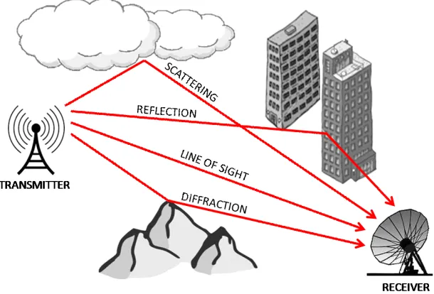
In a WC system, the propagation of signal does not rely on a specific path. Instead,
due to the existence of multiple paths, different copies of the same transmitted
sig-nal are received. Multiple paths can be generated, when the electromagnetic sigsig-nal
reflects to a larger surface, diffract from an irregular surface or experience scattering.
Fig. 1.6 shows multiple paths taken by a transmitted signal in a typical WC scenario.
The multiple received copies experience different fading due to their respective paths
and results in a non additive noise to the system in addition to AWGN. This
phe-nomenon is known as multipath or multi-channel fading. Multi-channel fading can be categorized [9] as
1. Flat slow fading- The signal bandwidth is smaller than the coherence bandwidth of the channel. The signal duration is smaller than the coherence time of the
channel.
2. Flat fast fading- The signal bandwidth is smaller than the coherence bandwidth of the channel. The signal duration is larger than the coherence time of the
channel.
3. Frequency selective slow fading - The signal bandwidth is larger than the co-herence bandwidth of the channel. The signal duration is smaller than the
coherence time of the channel.
4. Frequency selective fast fading - The signal bandwidth is larger than the coher-ence bandwidth of the channel. The signal duration is larger than the cohercoher-ence
time of the channel.
The error performance of different fading channels in studied in [23].
1.3.1.1 Rayleigh fading model
Here, we consider a multipath flat fading channel withM different transmission paths.
The total received signal along with AWGN n(t) is
r(t) =
M
∑
k=1
Akcos (ωct+θk) +n(t)
= cosωct M
∑
k=1
Akcosθk−sinωct M
∑
k=1
Aksinθk+n(t),
where Ak and θk are amplitude and phase of the signal of the k-th path. Due to the
uncertainty in the obstacle of the propagation path, the terms X = ∑Mk=1Akcosθk
and Y = ∑Mk=1Aksinθk are considered random variable (RV). For large number of
propagation paths i.e. for large values ofM, by central limit theorem [24] parameters
XandY are independent identically distributed (iid) Gaussian RV. Thus the envelope
of the received signalR =√X2 +Y2 follows a Rayleigh distribution with probability
distribution function (PDF)
fR(r) = r σ2e
−r
2
2σ2
, r ≥0, (1.6)
whereσ2 is the variance ofX andY. The RF signal in (1.2) can be represented by the
form given in (1.5) whererR=Xand rI =Y. It is shown earlier that r(t) = ℜ {˜r(t)}
where
˜
r(t) =
M
∑
k=1
Ak(cos (ωct+θk) +jsin (ωct+θk))
=
M
∑
k=1
Akej(ωct+θk)
=
M
∑
k=1
s|αk|ejθk
| {z }
baseband
ejωct.
This baseband signal after being sampled with a given sampling time Ts, yields the
baseband signal of the form
r=αs+n, (1.7)
whereαis a complex Gaussian RV with its amplitude|α|, a Rayleigh RV ands is the
transmitted baseband signal. The Rayleigh fading model is the most widely used for
simulating a WC channel with diverse modeling methods [25]. The performance of
different WC system models and modulation schemes have also been studied [26–29]
1.3.2
Carrier Frequency Offset
In every WC system, the baseband message signal is transmitted over a carrier signal
of a given frequency fc. This mechanism is known as modulation, which is already
discussed in section 1.2. In order to perfectly retrieve the baseband signal, the
oscilla-tor at the receiver should be ideally tuned to the frequency of the RF signal. However
in practical scenario, the two frequencies differ. This happens due to varied reasons
like Doppler shifts and device impairment causing physical differences between the
local oscillators of transmitter and receiver. This difference in the frequency is known
as CFO and can be expressed in the form
△f =fc−fr, (1.8)
wherefr is the frequency of the receiver oscillator. CFO introduces a frequency shift,
and the received signal in (1.5) becomes
r(t) =
M
∑
k=1
Akcos ((ωc+△ωc)t+θk) +n(t)
∴r˜(t) =
M
∑
k=1
Ak(cos ((ωc+△ωc)t+θk) +jsin ((ωc+△ωc)t+θk))
=
M
∑
k=1
Akej((ωc+△ωc)t+θk)
=
M
∑
k=1
s|αk|ejθkej△ωct
| {z }
baseband
ejωct,
which changes the relationship between the transmitted and received baseband signal
in (1.7) to the form
r=αsejϕ+n, (1.9)
where ϕ = 2π△f /fs is the carrier angular frequency offset (CAFO) and fs is the
symbol rate. The representation in (1.9) is valid when △fk ≪fs, which is typically
The advanced standards used in present day WC like long term evolution (LTE)
uses multi-carrier modulation schemes like orthogonal frequency division multiplexing
(OFDM) which relies greatly on the orthogonality between the sub-carriers. This
makes the system highly vulnerable to inter carrier interference (ICI) caused by CFO.
Practical systems suffer significant deterioration in performance with both
multi-channel fading and CFO as discussed in [31–34]. To mitigate this declension of QoS,
CFO has become a hot topic of study among researchers today.
1.4
Objective
The research is targeted to improve the QoS of WC systems affected by different
parameters introduced in section 1.3. Ideal detection algorithms are designed with an
assumption that the CSI is perfectly known to the receiver and it maintains frequency
synchronization with the transmitter. However, practical systems require estimating
the channel fading parameters and the CFO. The objective of the work presented
in the thesis is to design detection algorithms for a receive diversity system with
one transmit and multiple receive antenna in the presence of these estimation errors.
The aim is to achieve optimal detection of the transmitted message signal with the
erroneous estimates of CSI and CFO available to the receiver. The algorithms are
designed for three prevalent detection techniques and their performance is analyzed
in terms of BER.
1.5
Organization of Thesis
The rest of the thesis is organized as follows. In Chapter 2, a detailed review of
the prevalent detection techniques is introduced with their performance analysis for
ideal WC systems. Chapter 3 emphasizes on practical WC systems with CSI and
detection algorithms for three different techniques are derived in Chapter 4 and the
generalized form for these algorithms are also presented. Chapter 5 explains the
simulation method, for the analysis of performance of the proposed algorithms for
different modulation schemes. Experimental results are shown for different high values
of the estimation error variances. Chapter 6 summarizes the research along with
related ideas for future work. All relevant mathematical calculations required for
Chapter 2
SIMO Detection Techniques
MIMO, as discussed in chapter 1.1 is the most practically implemented system that
can effectively improve the QoS in the presence of multi-channel fading. Among
different diversity schemes discussed in chapter 1.1, receive diversity is shown to
yield high performance [11] with multiple antennas at the receiver. It is beneficial to
practically implement it, as the complex system with multiple antennas is installed
at the base station which already has a robust infrastructure. This makes the SIMO
system have a wide range of application [35–37] in different wireless systems. The
research presented in the thesis is primarily done for a two branch SIMO system
with one transmit and two receive antenna. This is further generalized for the cases
of multiple receive antennas. Fig. 2.1 demonstrates a simple block representation
of the working of a two branch SIMO model. The baseband message signal s is
modulated and the RF signal x(t) is propagated over the wireless channel using a
single transmit antenna. The signal after suffering attenuation due to multi-channel
fading and additive noise is received using two antennas. The received signal is further
demodulated and sampled to get the baseband signal at the k-th antenna as
rk=αks
√
Es+nk, (2.1)
where αk is the channel gain between the transmit antenna and the k-th receive
antenna, Es is the energy per symbol and nk is the zero mean AWGN with variance
σ2
n per dimension. This baseband signal is then passed through a detector block for
optimal estimation of the transmitted signal. The demapper then converts in into the
binary form of the original message or data signal. The main focus of the thesis will
be on the detector block at the receiver. The working of different detection schemes
for MIMO is explained in [38] and their performance is compared in [39]. The thesis
distinctively addresses ML decision detector, linear combiners and MMSE detector
for an ideal system ( ˆα = α), which are briefly introduced in section 2.4, section 2.2
and section 2.3 respectively.
2.1
Maximum Likelihood Detection
Maximum Likelihood is a method for detecting unknown parameters based on a set of
observations for a given statistic by maximizing the likelihood function. Considering
the system model presented in (2.1), the received signal rk and the channel fading
parameters αk from the k-th receive antenna are taken as the observations, whereas
the parameter to be detected is the transmitted signal s. Optimal detection is
ob-tained by choosing from a finite set of symbols X = {κ0,κ1, ...} of a given length,
depending on the type of modulation scheme. The aim is to obtain the optimum value
the observations is highest. This can be expressed as
s ,arg max
s∈X {P (s|rk, αk)}. (2.2)
The expression is known asmaximum a posteriori (MAP) probability function. Using Bayes’ theorem [24], (2.2) can be written in the form
s ,arg max
s∈X
{
P (s)P(rk|s, αk)
(rk)
}
, (2.3)
where the probability of receiving rk conditioned on αk and when s is transmitted,
P (rk|s, αk) is known as the likelihood function. Since we choose the value of s∈ X, P(s) is a constant and hence it can be seen from (2.3), that maximizing the likelihood
function maximizes the MAP probability. Thus the decision rule for optimal detection
becomes
s ,arg max
s∈X {P (rk|s, αk)}. (2.4)
The probability distribution of the received signal rk can be approximated to be of a
Gaussian RV as explained in [40]. The PDF of a Gaussian RV is of the form
f(r) = √1 2πσ2
r e
− |r−µr| 2
2σ2 r
, (2.5)
whereµr is the mean andσr2 is the variance. By taking the negative logarithm of the
likelihood function from (2.5), the decision metric in (2.4) becomes
s,arg min
s∈X {−logP (rk|s, αk)}
= arg min
s∈X
{
∥rk−αks∥2
}
.
(2.6)
For the case of a two branch SIMO, the ML decision metric for optimal detection of
the transmitted signal is
s,arg min
s∈X
{
|r0−α0s|2+|r1−α1s|2
}
. (2.7)
ML detection is widely in use for WC systems specially for MIMO. The performance
types of MIMO and other wireless systems. This technique has proved to be one of
the best in terms of minimizing the BER.
2.2
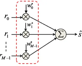
Linear Combiner
Diversity works, when M independent copies of the transmitted signal is received
from the array of M antennas at the receiver. The major challenge in receiver
diver-sity schemes is to effectively detect the data received by these antennas. Diverdiver-sity
combining works by dedicating the signals from the entire array of antennas to form
a single signal with the highest SNR. Thus they are more effective when the fading
suffered by the multiple copies of the received signal are independent. The most
prac-tical approach is linear combiners, for the simplicity of their implementation. Fig. 2.2
Figure 2.2: Linear Combiner
shows the working of a linear combiner and the generalized form is given as
ˆ
s=w0∗r0+w1∗r1+...+wM∗ −1rM−1, (2.8)
where w0, w1 and wM−1 are the weights for optimal combining of the received signal
r0, r1 and rM−1 respectively. Linear combiners are broadly categorized [5, 6] as the
following:
signal having the best SNR. The weight selection can be expressed as
w=
1 Γ = max
k {Γk}
0 otherwise
(2.9)
where Γ is the SNR of the signal.
2. Equal Gain Combining: This combining scheme assigns unit gain to all the signals. The general for of linear combiners in (2.8) becomes
ˆ
s=r0 +r1+...+rM−1, (2.10)
thus greatly reducing the computational complexity. But it is not an optimal
solution in terms of performance.
3. Maximal Ratio Combining: This combining scheme is said to provide op-timal solution in terms of SNR [6]. All the signals from the antenna array are
combined in a way that the resulting signal has the maximum SNR. The MRC
scheme is further discussed in detail.
An elaborate analysis of these combining schemes and their performance is done
in [45, 46].
2.2.1
Maximal Ratio Combiner
The general form for a linear combiner given in (2.8) reduced for a two branch SIMO
can be given as
ˆ
s =WHR, (2.11)
where W = [w0 w1]T are the combining weights or coefficients andR = [r0 r1]T are
the received signals at two antennas. From (2.1), the above relation can be written
as
ˆ
where Z = [α0 α1]T are the channel fading coefficients and N = [n0 n1]T is the
AWGN. Here, it is assumed that the receiver has perfect knowledge of CSI. The
instantaneous SNR can be expressed as
Γ =
E[WHZs2]
E[|WHN|2] = σ2
sWHZ 2
σ2 n∥W∥
2 . (2.13)
Here σ2
s and σn2 is the variance of the transmitted signal and the additive noise
re-spectively. Cauchy-Schwarz inequality [47] states the following relation
M∑−1
k=0 wkαk
2
≤
M∑−1
k=0
|wk| 2
M∑−1
k=0
|αk| 2
. (2.14)
Thus, maximum SNR can be obtained when W = Z. Substituting this relation
in (2.13) we get the maximum value of SNR
Γmax = σs2 σ2 n
∥Z∥2 = σ
2 s σ2 n
(
|α0| 2
+|α1| 2)
. (2.15)
Now, let us substitute the relation W = Z in the general form of linear
combin-ers (2.11), to get the expression for MRC
ˆ
s =ZHR
=α0∗r0+α1∗r1,
(2.16)
which is optimal in the sense of maximizing SNR.
2.2.2
ML Detector
ML decision is used after MRC for optimal detection of the transmitted signal in
terms of BER. For a two branch SIMO system optimal detection can be obtained by
choosing the value of s which can minimize the decision metric given in (2.7)
arg min
s
{
d2(r0, α0s) +d2(r1, α1s)
}
, (2.17)
whered2(x, y) is the squared euclidean distance between xand y which is calculated
as
Expanding (2.10) with little manipulation and substituting in (2.11), it can be easily
shown that the ML decision metric for optimal detection is
arg min
s
{(
α20+α21−1)|s|2+d2(ˆs, s)} (2.19)
and for equal energy constellations like PSK, the metric is reduced to
arg min
s
{
d2(ˆs, s)}. (2.20)
2.3
L-MMSE Detector
Linear MMSE detectors are designed for optimal detection of the transmitted signal
by minimizing the mean square error (MSE) between the original value and the
estimated value. For a WC system, the MMSE detector aims to minimize the MSE
between the transmitted signals and its MMSE estimate ˆs. Now, let us consider the
case of a two branch SIMO. The system model can be mathematically expressed in
the form
R=Zs+N, (2.21)
where R = [r0 r1]T are the received signals, Z = [α0 α1]T are the channel fading
coefficients and N = [n0 n1]T is the AWGN. The general form of a linear estimator
is the following
ˆ
s=KR (2.22)
and the MSE of the detector can be expressed as
J =E[∥s−sˆ∥2] (2.23)
Fig. 2.3 shows vector diagram depicting the relation between the original value,
esti-mate and MSE. Here, e is the error given by
Figure 2.3: Vector diagram of MSE
Orthogonality principle [48] states that an estimator achieves MMSE if and only if
the MSE is orthogonal to the observation. i.e. for Jmin,
e⊥R
⇒ E[eRH]= 0
⇒ E[(s−sˆ)RH]= 0
⇒ E[(s−KR)RH] = 0
⇒ K =E[sRH]E[RRH]−1.
(2.25)
Now, let us calculate it individually
E[RRH] =E
r0
r1
[ r0 r1 ]∗
=
σ2s|α0|2+σ2n 0
0 σ2
s|α1|2+σ2n
.
(2.26)
Similarly, we calculate
E[sRH] =E
[[
sr0∗ sr∗1
]]
=σ2s
[
α0∗ α∗1
]
.
(2.27)
Substituting the results of (2.26) and (2.27) in (2.25),
K =
σ2 sα∗0 σ2
s|α0|2+σn2
| {z }
σ2 sα∗1 σ2
s|α1|2+σn2
| {z }
Thus, from (2.22), we get the mathematical expression of linear MMSE detector for
a two branch SIMO as
ˆ
s=K0r0+K1r1, (2.29)
whereK0 and K1 can be obtained from (2.28). The performance of the linear MMSE
detector in terms of BER and computational complexity for different MIMO schemes
is studied in [49] and for the case of multiple users, in [50].
2.4
Performance Simulation for SIMO
This section presents a performance analysis of a two branch SIMO system. The
channel is assumed to be a Rayleigh fading channel and the transmitted symbols are
complex with QPSK modulation. It is also assumed that the detection of the
trans-mitted symbols is done with perfect knowledge of CSI at the receiver. There also
exits a perfect synchronization between the transmitter and receiver oscillators.
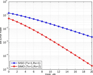
Fig. 2.4 shows the performance simulation of a two branch SIMO (one transmit
antenna and two receive antennas) having a classical MRC receiver, with a simple
system having no antenna diversity (one transmit antenna and one receive antenna).
It can be seen from the simulation result that SIMO system provides almost 6-dB
gain over the system with no diversity and the performance improves considerably
0 2 4 6 8 10 12 14 16 18 2020
10−5
10−4
10−3
10−2
10−1
100
SNR, dB
Bit Error Rate
SISO (Tx=1,Rx=1) SIMO (Tx=1,Rx=2)
Chapter 3
Effect of Imperfect Estimation
This section will focus on the effect of different parameter estimation errors on the
detection techniques reviewed in chapter 2. All derivations were done assuming that
the receiver is perfectly aware of the CSI and CFO. On the contrary, these parameters
are random and require to be estimated at the receiver. This problem has opened
doors to a lot of pioneering work to improve upon varying CSI and CFO estimation
techniques. However, it is impossible to achieve perfect estimation and thus the
detec-tion algorithms are no more optimal. In secdetec-tion 3.1, the effects of channel estimadetec-tion
error is discussed for all the three types of detection techniques and simulation results
are shown to compare the performance with an ideal system. Section 3.2 performs a
similar analysis with the effect of CFO estimation errors.
3.1
Imperfect Channel Estimation
Let us consider the two branch SIMO model discussed in the previous chapter. The
baseband signal at the k-th receive antenna as given in (2.1) is
rk=αks
√
Es+nk. (3.1)
Here, the channel fading parametersαk is assumed as a standard normal distribution,
estimator is assumed to be erroneous and regardless of the type of estimator used, it
can be modeled as
ˆ
αk =αk+ϵk, (3.2)
where ˆαk is the imperfect channel estimate and ϵk is the estimation error. Let us
consider the case of MMSE channel estimator where we transmit a set of pilot symbols
known to the receiver. The baseband signal in (3.1) during the training, can be
modified to show the relationship between the received signal and the pilots as
rk,t =αkpt+nk,t, (3.3)
where P = [p1 p2 ... pl] is the set of transmitted pilot symbols of length l and
rk = [rk,1 rk,2 ... rk,l] is the set of received observation at the k-th antenna. Thus
the MMSE estimate of the channel fading parameters can be obtained as
ˆ
αk = rkPH P PH
= rkP
H
∥P∥2.
(3.4)
Assuming that the pilot symbols are orthogonal to each other, we can easily write (3.3)
as
rkPH =αk∥P∥2+nkPH
⇒ αk = rkPH
∥P∥2 − nkPH
∥P∥2
⇒ αˆk =αk+ nkPH
∥P∥2
| {z }
ϵk .
(3.5)
This relation is similar to the one assumed in [51, 52]. The channel estimation ϵk ∼
N(0, σ2
ϵ) is considered a zero mean Gaussian RV with varianceσ2ϵ. Using the relation
in (3.2), it can be easily concluded that the imperfect estimate ˆαk ∼ N(0, σ2αˆ) is
also a Gaussian RV with mean zero and variance σ2 ˆ
α. The error performance of
in [53–55]. It is proven mathematically, that the estimation error prevents the receiver
to achieve optimal detection of the transmitted signal and there by deteriorating the
system performance.
3.1.1
ML Detector
ML detector discussed in section 2.4 leads to choosing the optimal value of the
trans-mitted symbol s by maximizing the MAP function
s ,arg max
s∈X {P (s|rk, αk)}. (3.6)
However in this case, the estimator at the receiver shown in Fig. 3.1 provides
imper-Figure 3.1: ML detector with channel estimator
fect estimate of the channel parameters ˆαkwhich is given as an input to the detector.
This makes the decision metric
s ,arg max
s∈X {P (s|rk,αˆk)}. (3.7)
By Bayes’ theorem introduced earlier, the decision metric leads to maximizing the
likelihood function
s ,arg max
Taking negative logarithm and using the relation in (3.2), the ML decision metric is
given in the form
s,arg min
s∈X
{
|r0−αˆ0s|2+|r1 −αˆ1s|2
}
= arg min
s∈X
{
|r0−(α0+ϵ0)s|2+|r1−(α1+ϵ1)s|2
}
.
(3.9)
This form of ML detection metric involves the channel estimation error ϵk and does
not provide optimal detection. The degradation of the system performance will be
further analyzed by simulation in section 3.1.4.
3.1.2
Linear Combiner
Among all linear combiners, MRC is shown in section 2.2 as the most optimal
com-biner in the sense of maximizing the SNR of its output. Taking, the general equation
of a linear combiner from (2.8), we get
ˆ
s=w0∗r0+w1∗r1+...+wM∗ −1rM−1. (3.10)
It is shown in section 2.2.1, that the maximum value of combiner output SNR can
be obtained when wk = αk. Fig. 3.2 shows that the channel estimates ˆαk known to
the receiver is used by the combiner and the MRC scheme becomes
ˆ
s= ˆα∗0r0+ ˆα∗1r1
= (α0+ϵ0)∗r0+ (α1+ϵ1)∗1r1,
(3.11)
which does not provide an output with the maximum SNR and hence is not optimal.
Moreover, the ML detector block with the imperfect channel estimates minimizes the
decision metric
s,arg min
s
{(
ˆ
α20+ ˆα21−1)|s|2+d2(ˆs, s)}
= arg min
s
{(
(α0+ϵ0)2+ (α1+ϵ1)2−1
)
|s|2+d2(ˆs, s)}.
(3.12)
Mathematical model of the BER performance and the SNR of the combiner output is
derived in [56–60]. It is shown that the performance of a linear combiner aggravates
significantly in the presence of channel estimation error.
3.1.3
L-MMSE
MMSE detector introduced in section 2.3, is one of simplest of all linear estimators
and optimal in the sense of minimizing the BER. The MMSE form derived in (2.29)
Figure 3.3: MMSE detector with channel estimator
has the coefficient vector K given in (2.28) as
K =
[
σ2sα∗0 σ2|α |2+σ2
σs2α∗1 σ2|α |2+σ2
]
If we substitute the channel parameters in (3.13) with the estimates as shown in
Fig. 3.3, the coefficient vector becomes
K =
[
σ2 sαˆ∗0 σ2
s|αˆ0| 2
+σ2 n
σ2 sαˆ∗1 σ2
s|αˆ1| 2
+σ2 n ] = σ2
s(α0+ϵ0)∗ σ2
s|(α0+ϵ0)| 2
+σ2 n
| {z }
K0
σ2
s(α1 +ϵ1)∗ σ2
s|(α1+ϵ1)| 2
+σ2 n
| {z }
K1
.
(3.14)
It is shown in [61–63] that MMSE detector with the above coefficient does not provide
optimal detection.
3.1.4
Performance Simulation
In this section, the performance of a two branch SIMO system is analyzed in the
presence of channel estimation error. The channel is assumed to be a Rayleigh
fad-ing channel with its parameters havfad-ing mean zero and unit variance. The channel
estimator is taken as a MMSE estimator, as explained earlier in this section and the
estimation model ˆαk=αk+ϵkfrom (3.5). Let us assume that variance of the AWGN
is σn2 =N0. Thus as described in [51], by Cramer-Rao bound the minimum value of
the estimation error variance is
σϵ2 = N0
lEs
, (3.15)
where l is the length of pilot symbols transmitted during training. The simulation
is performed by transmitting 104 frames of data symbols with a frame length of 130
symbols. The results are analyzed by plotting the BER against multiple values of
SNR. The SNR is defined as σ2
s/σ2n where σs2 is taken to be unity. The performance
is analyzed for multiple values of the estimation error variances by varying the length
0 1 2 3 4 5 6 7 8
10−2
10−1
SNR, dB
Bit Error Rate
l = 4
l = 8
l = 16 Ideal
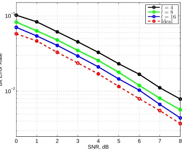
Figure 3.4: Performance of 4-PSK SIMO with channel estimation error
Fig. 3.4 demonstrates the performance of 4-PSK or QPSK modulation scheme in
the presence of channel estimation error. It is shown that the performance
depreci-ates for higher values of estimation error and suffers almost 2-dB loss in SNR for a
0 1 2 3 4 5 6 7 8
10−2
10−1
SNR, dB
Bit Error Rate
l = 4
l = 8
l = 16 Ideal
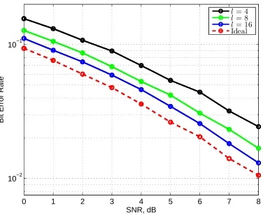
Figure 3.5: Performance of 8-PSK SIMO with channel estimation error
Fig. 3.5 demonstrates the performance of 8-PSK modulation scheme in the
pres-ence of channel estimation error. It is shown that the performance suffers almost
2.5-dB loss in SNR for a given BER. It is known from standard literature that the
BER performance depreciates for higher modulation schemes. In the presence of
0 1 2 3 4 5 6 7 8
10−1
SNR, dB
Bit Error Rate
l = 4
l = 8
l = 16 Ideal
Figure 3.6: Performance of 16-PSK SIMO with channel estimation error
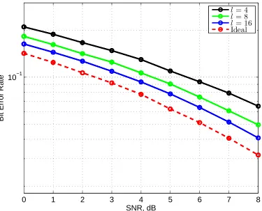
Fig. 3.6 demonstrates the performance of 16-PSK modulation scheme in the
pres-ence of channel estimation error. It is shown that the performance suffers almost
3-dB loss in SNR for a given BER. The performance deteriorates from 8-PSK
0 1 2 3 4 5 6 7 8
10−2
10−1
SNR, dB
Bit Error Rate
l = 4
l = 8
l = 16 Ideal
Figure 3.7: Performance of 4-QAM SIMO with channel estimation error
Fig. 3.7 demonstrates the performance of 4-QAM modulation scheme in the
pres-ence of channel estimation error. It is shown that the performance suffers almost
2-dB loss in SNR for a given BER and demonstrates identical performance as that of
0 1 2 3 4 5 6 7 8
10−1
100
SNR, dB
Bit Error Rate
l = 4
l = 8
l = 16 Ideal
Figure 3.8: Performance of 16-QAM SIMO with channel estimation error
Fig. 3.8 demonstrates the performance of 16-QAM modulation scheme in the
pres-ence of channel estimation error. It is shown that the performance suffers almost
7-dB loss in SNR for a given BER. The performance aggravates highly as compared
0 1 2 3 4 5 6 7 8
10−1
100
SNR, dB
Bit Error Rate
l = 4
l = 8
l = 16 Ideal
Figure 3.9: Performance of 64-QAM SIMO with channel estimation error
Fig. 3.9 demonstrates the performance of 64-QAM modulation scheme in the presence
of channel estimation error. It is shown that the performance suffers over 10-dB loss in
SNR for a given BER. This modulation scheme maps 16 symbols to one constellation,
3.2
Imperfect CFO Estimation
The optimal detection of the transmitted signal can be done, when the RF signal is
perfectly demodulated. This requires the frequency of the receiver oscillator to be in
perfect synchronization with the carrier frequency of the transmitted RF signal. It
is discussed in section 1.3.2, that in practical systems there is a mismatch in the two
frequencies. This mismatch is known as CFO and its mathematical relation is given
in (1.8). Thus, for a system affected by CFO, the received baseband signal at the
k-th antenna is
rk =αksejϕk
√
Es+nk, (3.16)
where ϕ = 2π△f /fs is the CAFO which is assumed to be a Gaussian RV with zero
mean and variance σ2
ϕ, similar to the assumptions made in [64, 65]. The CAFO is
unknown to the receiver and is estimated before detection. Irrespective of the type
of estimator, the CAFO estimate ˆϕk is modeled same as that of the channel estimate
in (3.2).
ˆ
ϕk=ϕk+εk (3.17)
The estimation error εk ∼ N(0, σ2ε) is considered a zero mean Gaussian RV. Since,
the original value of CAFO ϕk and the estimation error εk are independent of each
other, the imperfect estimate is also a Gaussian RV ˆϕk ∼ N
(
0, σ2 ˆ ϕ
)
. In this section,
we consider the most general practical case of a system, in the presence of both CSI
and CFO estimation. The system performance highly degrades with effect of these
imperfect estimates and its detailed analysis is given in [66–69]. It is also shown using
simulation, later in this section.
3.2.1
ML Detector
The ML detector in the presence of channel estimation error maximizes the decision
changes the decision metric for choosings ∈ X, to
s,arg max
s∈X
{
P
(
s|rk,αˆk,ϕˆk
)}
. (3.18)
Figure 3.10: ML detector with channel and CFO estimator
Thus by Bayes’ theorem, the likelihood function is
s,arg max
s∈X
{
P
(
rk|s,αˆk,ϕˆk
)}
. (3.19)
Using the baseband representation in (3.16), the ML detector in the presence of both
channel and CFO estimation error becomes
s,arg min
s∈X
{
r0−αˆ0sej ˆ ϕ0
2
+r1−αˆ1sej ˆ ϕ1
2}
= arg min
s∈X
{
r0−(α0+ϵ0)sej(ϕ0+ε0) 2
+r1−(α1+ϵ1)sej(ϕ1+ε1) 2}
.
(3.20)
The presence of estimates ˆαk and ˆϕk of CSI and CAFO respectively does not provide
optimal detection. The performance of the ML detector under the mismatch scenario
is simulated in section 3.2.4.
3.2.2
Linear Combiner
The combiner relation in (3.11) is derived for imperfect estimates of the channel.
Figure 3.11: MRC with channel and CFO estimator
combiner becomes
ˆ
s= ˆα∗0e−jϕˆ0r
0+ ˆα∗1e− jϕˆ1r
1
= (α0+ϵ0)∗e−j(ϕ0+ε0)r0+ (α1+ϵ1)∗1e−j(ϕ1+ε1)r1,
(3.21)
which deteriorates the output SNR of the combiner. The effect of CFO estimation
error is studied and analyzed for diversity combiners in [66]. However, the ML detector
given in (3.12) remains the same and has no effect on its performance by the erroneous
CFO estimation.
3.2.3
L-MMSE
The linear MMSE detector derived in (3.14), is in the presence of channel estimation
error and it is shown to be no more optimal. As given in Fig. 3.12, in this case the
Figure 3.12: MMSE detector with channel and CFO estimator
the MMSE coefficients can be written as
K =
[
σ2 sαˆ∗0e−j
ˆ ϕ0
σ2
s|αˆ0|2+σn2 σ2
sαˆ∗1e−j ˆ ϕ1
σ2
s|αˆ1|2+σ2n
] = σ2
s(α0+ϵ0)∗e−j(ϕ0+ε0) σ2
s|(α0+ϵ0)|2+σ2n
| {z }
K0
σ2
s(α1+ϵ1)∗e−j(ϕ1+ε1) σ2
s|(α1+ϵ1)|2+σn2
| {z }
K1
.
(3.22)
The detail analysis of the performance degradation is done in [70].
3.2.4
Performance Simulation
In this section the performance of a two branch SIMO is analyzed in the presence of
both CSI and CFO estimation errors. Similar setup is assumed as that of section 3.1.4.
The CAFO estimate is modeled as ˆϕk =ϕk+εk. The variance of CAFO estimation
error is considered a simple multiple of the AWGN variance given as
σε2 =aσn2 (3.23)
where a is any integer. A channel estimator is also assumed with an error variance
given in (3.15) with the length of the pilot symbolsl= 16. Only the CAFO estimation
error variance, is altered by the adopting the valuesa= 1, 4 and 9. A comparison is
0 1 2 3 4 5 6 7 8
10−2
10−1
SNR, dB
Bit Error Rate
a= 1
a= 4
a= 9 Known CFO
Figure 3.13: Performance of 4-PSK SIMO with CSI and CFO estimation error
Fig. 3.13 demonstrates the performance of 4-PSK or QPSK modulation scheme in
the presence of both CSI and CFO estimation error. It is shown that the
0 1 2 3 4 5 6 7 8
10−2
10−1
SNR, dB
Bit Error Rate
a= 1
a= 4
a= 9 Known CFO
Figure 3.14: Performance of 8-PSK SIMO with CSI and CFO estimation error
Fig. 3.14 demonstrates the performance of 8-PSK in the presence of both CSI and
CFO estimation error. It is shown that the performance suffers over 10-dB loss in
SNR for a given BER. For higher error variance of the CFO, the performance
0 1 2 3 4 5 6 7 8
10−1
SNR, dB
Bit Error Rate
a= 1
a= 4
a= 9 Known CFO
Figure 3.15: Performance of 16-PSK SIMO with CSI and CFO estimation error
Fig. 3.15 demonstrates the performance of 16-PSK in the presence of both CSI and
CFO estimation error. It is shown that the performance degrades further than the
8-PSK modulation scheme and suffers a comparatively higher loss than the QPSK
0 1 2 3 4 5 6 7 8
10−2
10−1
SNR, dB
Bit Error Rate
a= 1
a= 4
a= 9 Known CFO
Figure 3.16: Performance of 4-QAM SIMO with CSI and CFO estimation error
Fig. 3.16 demonstrates the performance of 4-QAM in the presence of both CSI and
CFO estimation error. The performance demonstrated by this modulation scheme,
0 1 2 3 4 5 6 7 8
10−1
SNR, dB
Bit Error Rate
a= 1
a= 4
a= 9 Known CFO
Figure 3.17: Performance of 16-QAM SIMO with CSI and CFO estimation error
Fig. 3.17 demonstrates the performance of 16-QAM in the presence of both CSI and
CFO estimation error. This scheme maps 4 symbols per constellation. It is shown by
0 1 2 3 4 5 6 7 8
100
SNR, dB
Bit Error Rate
a= 1
a= 4
a= 9 Known CFO
Figure 3.18: Performance of 64-QAM SIMO with CSI and CFO estimation error
Fig. 3.18 demonstrates the performance of 64-QAM in the presence of both CSI
and CFO estimation error. This scheme maps 16 symbols per constellation. The