University of Windsor University of Windsor
Scholarship at UWindsor
Scholarship at UWindsor
Electronic Theses and Dissertations Theses, Dissertations, and Major Papers
10-19-2015
The Effects of Uncertainty in Engineering Data on the Design and
The Effects of Uncertainty in Engineering Data on the Design and
Performance of Automotive Thermal Systems
Performance of Automotive Thermal Systems
Ashley Nicole Lehman
University of Windsor
Follow this and additional works at: https://scholar.uwindsor.ca/etd
Recommended Citation Recommended Citation
Lehman, Ashley Nicole, "The Effects of Uncertainty in Engineering Data on the Design and Performance of Automotive Thermal Systems" (2015). Electronic Theses and Dissertations. 5459.
https://scholar.uwindsor.ca/etd/5459
This online database contains the full-text of PhD dissertations and Masters’ theses of University of Windsor students from 1954 forward. These documents are made available for personal study and research purposes only, in accordance with the Canadian Copyright Act and the Creative Commons license—CC BY-NC-ND (Attribution, Non-Commercial, No Derivative Works). Under this license, works must always be attributed to the copyright holder (original author), cannot be used for any commercial purposes, and may not be altered. Any other use would require the permission of the copyright holder. Students may inquire about withdrawing their dissertation and/or thesis from this database. For additional inquiries, please contact the repository administrator via email
The Effects of Uncertainty in Engineering Data on the Design and Performance of Automotive Thermal Systems
By
Ashley Nicole Lehman
A Thesis
Submitted to the Faculty of Graduate Studies
through the Department of Mechanical, Automotive, and Materials Engineering
in Partial Fulfillment of the Requirements for the Degree of Master of Applied Science
at the University of Windsor
Windsor, Ontario, Canada
2015
The Effects of Uncertainty in Engineering Data on the Design and Performance of Automotive Thermal Systems
by
Ashley Nicole Lehman
APPROVED BY:
______________________________________________ Dr. D. Green
Engineering Materials
______________________________________________ Dr. J. Johrendt
Mechanical Engineering
______________________________________________ Dr. V. Stoilov, Co-Advisor
Mechanical Engineering
______________________________________________ Dr. A. Sobiesiak, Co-Advisor
Mechanical Engineering
iii
DECLARATION OF ORIGINALITY
I hereby certify that I am the sole author of this thesis and that no part of this thesis has been published or submitted for publication.
I certify that, to the best of my knowledge, my thesis does not infringe upon anyone’s copyright nor violate any proprietary rights and that any ideas, techniques, quotations, or any other material from the work of other people included in my thesis, published or otherwise, are fully acknowledged in accordance with the standard referencing practices. Furthermore, to the extent that I have included copyrighted material that surpasses the bounds of fair dealing within the meaning of the Canada Copyright Act, I certify that I have obtained a written permission from the copyright owner(s) to include such material(s) in my thesis and have included copies of such copyright clearances to my appendix.
iv
ABSTRACT
This study has two purposes: (1) to investigate the effects of uncertainty on
thermal design and performance (2) to establish a process to couple the results
from uncertainty analysis with Design for Six Sigma (DFSS) to improve
robustness. The research was conducted with support from FCA group. The
analysis was applied to a component selected by FCA group; however, it is
applicable to any system.
The effects of uncertainty were investigated using the Fourier Amplitude
Sensitivity Test (FAST). The analysis was run on MATLAB software package
using estimated uncertainty ranges for each parameter. The parameters with the
greatest influence on thermal performance uncertainty were identified.
These parameters were used as control factors in a DFSS study. The thermal
performance was simulated on RadTherm software package with several settings
for the critical parameters. The settings which allowed the performance to remain
v
DEDICATION
This thesis is dedicated to my parents, who have always supported me, and took
care of Scooby while I was away for the year.
I would also like to dedicate this thesis to my boyfriend, Thomas, for always being
there for me and making me laugh in the stressful times.
And finally, I would like to dedicate this thesis to Scott, Yvette, & Leto, for
providing me with the greatest inspiration to complete this work while I was in
vi
ACKNOWLEDGEMENTS
There are many people who I would like to sincerely thank for making this thesis
possible.
First, I would like to sincerely thank my University of Windsor advisor, Dr.
Stoilov, for teaching me and making sure I had everything I needed to be
successful. I definitely could not have completed this thesis without the extra effort
and time you put in to help me and I am very thankful to you.
I would also like to thank my industrial advisors, Alaa El-Sharkawy, Richard Sun
& Enrico Ribaldone, for your kindness and helpfulness throughout the past two
years. I learned a great deal from you and I appreciate everything you did to help
me complete this thesis.
I would like to thank my supervisors from the Politecnico di Torino, Professor
Ezio Spessa and Professor Daniela Misul, for taking the time to meet with me and
review my progress while I was in Italy. You helped me to stay on track and gave
me helpful advice for improving this thesis.
Finally, I would like to sincerely thank the Mitacs-Accelerate Program for
providing the financial support which made this research project possible. The
Mitacs-Accelerate Program provided me with a truly exceptional learning
vii
TABLE OF CONTENTS
DECLARATION OF ORIGINALITY ... iii
ABSTRACT ... iv
DEDICATION ... v
ACKNOWLEDGEMENTS ... vi
LIST OF TABLES ... x
LIST OF FIGURES ... xii
LIST OF APPENDICES ... xiv
LIST OF ABBREVIATIONS/SYMBOLS ... xv
CHAPTER 1 PURPOSE AND SIGNIFICANCE OF THE STUDY ... 1
Purpose ... 1
Significance ... 2
CHAPTER 2 LITERATURE REVIEW ... 2
CHAPTER 3 SELECTION OF CASE STUDY OF A SPECIFIC UNDERBODY COMPONENT WHICH HAS SIGNIFICANT INTEREST TO THE COMPANY AND AERO/THERMAL ORGANIZATION ... 15
CHAPTER 4 APPLICATION OF THE FOURIER AMPLITUDE SENSITIVITY TEST (FAST) METHOD TO AN UNDERBODY COMPONENT ... 19
Fourier Amplitude Sensitivity Test (FAST) ... 19
Analytical Model Development ... 20
Energy Balance Equations ... 21
Energy Balance for the Lower Layer of the Heat Shield ... 28
viii
Energy Balance for the Spare Tire Tub ... 42
Approximation of Nominal Values of Input Parameters ... 46
Effects of Uncertainty on Thermal Performance ... 49
Evaluation of Uncertainty of Input Parameters ... 53
Convection Heat Transfer Coefficients ... 53
Reynolds Number (for Airflow over Lower Surface of Heat Shield) Uncertainty Analysis ... 59
CHAPTER 5 DEVELOPMENT OF A METHOD TO INTERFACE THE RESULTS FROM FAST WITH DESIGN FOR SIX SIGMA (DFSS) TO ACHIEVE ROBUST DESIGN FOR THERMAL PROTECTION... 72
Step 1 – Identify Opportunity ... 72
Step 2 – Robust Optimization ... 74
Control Factors and Levels ... 80
Optimization Results ... 92
Prediction of Optimal Design ... 96
Step 3 – Confirmation of DFSS Optimal Design Predictions ... 100
CHAPTER 6 CONCLUSIONS ... 104
REFERENCES/BIBLIOGRAPHY... 108
APPENDICES ... 110
Reynolds Number (for Airflow over Upper Surface of Heat Shield) Uncertainty Analysis ... 114
ix
x
LIST OF TABLES
Table 1 - Input Parameters for the Analytical Model Developed to Implement the
FAST Method ... 22
Table 2 - L4 Orthogonal Array ... 78
Table 3 - Levels of the Emissivity of the Heat Shield ... 81
Table 4 - Levels of the Emissivity of the Muffler ... 82
Table 5 - Levels of the Density of the Heat Shield ... 83
Table 6 - Levels of the Specific Heat Capacity of the Spare Tire Tub ... 83
Table 7 - Levels of the Thickness of the Spare Tire Tub ... 84
Table 8 - Levels of the Thickness of the Outer Layers of the Heat Shield ... 85
Table 9 - Control Factors and Levels ... 85
Table 10 - Noise Factors ... 86
Table 11 - Input Signal ... 87
Table 12 - Orthogonal Array for N1 (Worst-Case Noise) and M1 (Worst-Case Input Signal) Condition... 88
Table 13 - Orthogonal Array for N1 (Worst-Case Noise) and M2 (Best-Case Input Signal) Condition ... 89
Table 14 - Orthogonal Array for N2 (Best-Case Noise) and M1 (Worst-Case Input Signal) Condition ... 90
Table 15 - Orthogonal Array for N2 (Best-Case Noise) and M2 (Best-Case Input Signal) Condition ... 91
xi
Table 17 - Signal-to-Noise Ratios Calculated for Each Control Factor at Each
Level ... 97
Table 18 - Confirmation Runs for Optimal S/N Ratio and Optimal Slope of
Best-Fit Line ... 101
xii
LIST OF FIGURES
Figure 1 - Many Sources of Uncertainty Exist for the Thermal Performance of
Underbody Components Resulting in an Unpredictable Thermal System ... 18
Figure 2 - Sketch of Underbody Components Considered in the Analytical Model ... 21
Figure 3 - Energy Balance of Lower Layer of Heat Shield ... 29
Figure 4 - Energy Balance of Upper Layer of Heat Shield... 35
Figure 5 - Energy Balance of Spare Tire Tub ... 42
Figure 6 - Partial Variance of Input Parameters for Low, Medium, and High Uncertainty ... 50
Figure 7 - Partial Variance of Control Parameters at Low, Medium, and High Uncertainty ... 52
Figure 8 - Partial Variance of Input Parameters Using Estimated Uncertainty for Each Input Parameter ... 69
Figure 9 - Partial Variance of Control Parameters Using Estimated Uncertainty for Each Input Parameter ... 70
Figure 10 - Partial Variance of Control factors Using Estimated Uncertainty for Each Input Parameter ... 71
Figure 11 - Comparison between the Current Design and the Ideal Design ... 73
Figure 12 - DFSS P-Diagram (Parametric Diagram) ... 77
xiii
Figure 14 - Slope of Best-Fit Line, β, Calculated for Each Control Factor at Each
Level ... 98
Figure 15 - Signal-to-Noise Ratio Response Graph ... 99
Figure 16 – Slope of Best-Fit Line Response Graph ... 99
Figure 18 - Ideal Function Chart with Ideal Design, Current Design, and
xiv
LIST OF APPENDICES
Appendix A - Calculation of Uncertainty Range for Heat Transfer Coefficient for
Air Flow over Upper Surface of Heat Shield and Spare Tire Tub ... 110
xv
LIST OF ABBREVIATIONS/SYMBOLS
FAST Fourier Amplitude Sensitivity Test
DFSS Design for Six Sigma
𝑐𝑠𝑡 Specific heat capacity of spare tire tub
𝑐ℎ𝑠_𝑜 Specific heat capacity of outer layers of heat shield
𝐷1𝑚 Diameter 1 of muffler
𝐷2𝑚 Diameter 2 of muffler
𝜀𝑚 Emissivity of muffler
𝜀𝑠𝑡 Emissivity of spare tire tub
𝜀ℎ𝑠 Emissivity of heat shield
ℎ𝑠𝑡 Heat transfer coefficient for air flow over spare tire tub
ℎℎ𝑠𝑙 Heat transfer coefficient for air flow over lower surface of heat shield
ℎℎ𝑠𝑢 Heat transfer coefficient for air flow over upper surface of heat shield
𝑘ℎ𝑠_𝑖 Thermal conductivity of inner layer of heat shield
𝐿𝑠𝑡 Length of spare tire tub
𝐿ℎ𝑠 Length of heat shield
𝐿ℎ𝑠_𝑠𝑡 Clearance between heat shield and spare tire tub
𝐿𝑚_ℎ𝑠 Clearance between muffler and heat shield
xvi 𝜌ℎ𝑠_𝑜 Density of outer layers of heat shield
𝑇𝑚 Temperature of muffler surface
𝑇𝑎ℎ𝑠𝑢 Temperature of air flow over upper surface of heat shield
𝑇𝑎ℎ𝑠𝑙 Temperature of air flow over lower surface of heat shield
𝑇𝑎𝑠𝑡 Temperature of air flow over spare tire tub
𝑡𝑠𝑡 Thickness of spare tire tub
𝑡ℎ𝑠_𝑜 Thickness of outer layers of heat shield
𝑡ℎ𝑠_𝑖 Thickness of inner layer of heat shield
𝑊𝑠𝑡 Width of spare tire tub
𝑊ℎ𝑠 Width of heat shield
S/N Signal-to-noise ratio
r Sum of squares of the input (signal factor levels)
β Slope of best-fit line
𝑆𝛽 Sum of squares of distance between zero and the least square best fit line (Forced
through zero) for each data point
𝑆𝑒 Sum of squares of distance between individual data point to the least square best
fit line
𝑆𝑇 Sum of squares of distance between zero to each data point
𝑉𝑒 Variance
1
CHAPTER 1
PURPOSE AND SIGNIFICANCE OF THE STUDY
Purpose
The objective of this project is to study the effects of uncertainty on the thermal design
process. This project is focused on the uncertainty in design parameters which affect heat
transfer to the underbody components which are in the direct radiation view path of the
exhaust system. However, the goal of this investigation is to produce an uncertainty
analysis method which is applicable to any system.
Through this analysis, a greater understanding of uncertainty with respect to thermal
protection will be achieved. Once the uncertainty in the design parameters has been
studied, the Fourier Amplitude Sensitivity Test (FAST) will be applied to understand
which parameter’s uncertainty has the greatest influence on the uncertainty in the thermal
performance of the system. Thus, the most critical design parameters can be identified.
Another objective of this project is to develop a method to interface the results from
uncertainty analysis with Design for Six Sigma (DFSS). This method should allow for the
determination of the best settings for the most influential design parameters to improve
system robustness. In this specific case study, the goal is to improve thermal performance
of vehicle components which are exposed to high thermal loads. In the future, this
methodology may be applied to other systems to improve robustness in the early design
stages. The main advantage of this process is that it can be used to pinpoint potential
2
Significance
Uncertainty analysis has not been widely used in the study of computational model
uncertainty in the automotive industry (El-Sharkawy A. , Sensitivity and Uncertainty
Analysis in Computational Thermal Models, 2014). This study aims to analyze the
uncertainty in computational models and develop a method so that it may be further
applied to other automotive applications.
CHAPTER 2
LITERATURE REVIEW
Uncertainty is an inherent part of the design process. Every measurement, experiment,
and simulation depends on parameters which are uncertain; therefore, they provide
uncertain results. Engineers conduct uncertainty analysis to understand how uncertainty
affects the performance of products and processes. In “Experimentation and Uncertainty
Analysis for Engineers” (Coleman & Steele, 1999) an interesting example of uncertainty
analysis is highlighted involving lignite samples. In this example, an experiment is
conducted using a bomb calorimeter to find the heating value of a one gram sample of
lignite. The experimenters are able to find the heating value of this sample with
uncertainty less than two percent. However, there is a significant amount of variation
within a sample of lignite and even more variation between different samples of lignite.
Thus, the uncertainty arises not from the measurement technique but rather from the
variation within the physical variable itself. Coleman & Steele pose the question, “What
is the uncertainty in the lignite heating value?” They conclude that the uncertainty
3
the accuracy of a particular measurement; however, it can also be used to investigate the
entire range of potential values which may exist for a parameter.
Sensitivity and uncertainty analysis allow the engineer to understand the sources of
uncertainty in the input parameters and discover ways to reduce the amount of
uncertainty in the performance of the product or system. For example, after performing
an uncertainty analysis, an engineer may find that the variation in the thickness of a heat
shield for a component causes the temperature of that component to vary significantly
and to frequently exceed the specification. With this information, the engineer can
evaluate whether the tolerances for the heat shield should be tightened or if the nominal
value of the thickness of the heat shield should be increased. Both of these methods will
cause the component temperature to become more robust, meaning that it will remain
consistent regardless of variation in other parameters. By improving robustness, the
engineer ensures that the component remains within the specifications and therefore will
always meet the customer requirements.
An example of the benefits of uncertainty analysis is shown in the SAE paper, “Analysis
of Thermocouple Temperature Response under Actual Vehicle Test Conditions”
(El-Sharkawy A. E., Analysis of Thermocouple Temperature Response under Actual Vehicle
Test Conditons, 2008). In this case, the uncertainty in temperature measurements made
by thermocouples during vehicle testing is investigated. These temperature measurements
are used as a basis for design decisions; therefore, it is very important that they are
4
The uncertainty in these temperature measurements is due to radiation from the exhaust,
ambient temperature, and air flow. To combat these sources of uncertainty, El-Sharkawy
points out that the method of thermocouple installation must be carefully controlled.
Installing the thermocouple on the outer surface of the component risks errors due to the
difference in emissivity between the thermocouple and the component. The disparity in
emissivity may cause a difference between the amount of radiation heat transfer which
occurs between the surroundings and the component and the surrounding and the
thermocouple. Installing the thermocouple too far within the component may cause the
thermocouple to measure a lower temperature than the surface temperature if the
component is made of a material with low thermal conductivity. To understand exactly
where the thermocouple should be installed to obtain accurate temperature
measurements, an uncertainty analysis must be applied.
The uncertainty analysis begins with the development of an analytical model for the
transient response of the thermocouple. El-Sharkawy applies an energy balance to the
thermocouple junction.
Equation 1
𝑚𝑐𝑐𝑝
𝜕𝑇𝑐
𝜕𝑡 = ℎ𝐴(𝑇𝑎𝑖𝑟 − 𝑇𝑐) + 𝜎𝜀𝐹𝐴(𝑇𝑒𝑥ℎ
4− 𝑇
𝑐4) − 𝑘𝑐𝐴
𝜕𝑇𝑐 𝜕𝑟
Where:
𝑚𝑐: mass of thermocouple junction
𝑐𝑝: specific heat capacity of thermocouple junction
5
𝑇𝑎𝑖𝑟: temperature of ambient air
ℎ: heat transfer coefficient between air flow and thermocouple junction
𝐴: surface area of thermocouple junction (available for heat exchange with ambient)
𝑘𝑐: thermal conductivity of thermocouple junction
𝑟: radius of thermocouple junction
This energy balance considers convection from air flow, conduction through the
thermocouple junction, and radiation from the exhaust surface.
Next, the conduction is neglected based on the transient response time of a spherical
thermocouple which is calculated to be approximately ten seconds. In typical automotive
testing procedures, the sampling time is five to ten seconds. Therefore, this response time
is considered fast enough to neglect the conduction resistance. Under steady-state
conditions, the energy balance becomes:
Equation 2
0 = ℎ𝐴(𝑇𝑎𝑖𝑟− 𝑇𝑐) + 𝜎𝜀𝐹𝐴(𝑇𝑒𝑥ℎ4− 𝑇𝑐4)
Equation 3
(𝑇𝑐− 𝑇𝑎𝑖𝑟) =𝜎𝜀𝐹(𝑇𝑒𝑥ℎ
4− 𝑇
𝑐4)
ℎ
Therefore, El-Sharkawy defines the error between the actual temperature and the
6
Equation 4
𝐸𝑟𝑟𝑜𝑟 = (𝜎𝜀𝐹
ℎ ) (𝑇𝑒𝑥ℎ
4− 𝑇
𝑐4)
Based on this equation, it can be concluded that the error is strongly dependent on the
heat source temperature and inversely proportional to the heat transfer coefficient.
Therefore, El-Sharkawy concludes that when the vehicle is not heavily loaded and there
is high air flow, the thermocouple error will be lower. Contrastly, when the vehicle is
heavily loaded, the error will be high. Also, the emissivity of the thermocouple has a
direct impact on the error. Typically, the emissivity of the thermocouple junction is
between 0.2 and 0.3. However, if the surface of the junction is oxidized or if carbon or
soot accumulates on the surface, the emissivity will increase to 0.9 or 1. In this case, the
error will be much higher.
El-Sharkawy explains that thermal testing is usually conducted at high loads and speeds,
where radiation can be very significant, and therefore the error in the thermocouple
reading can reach up to 40%. Based on this approximation of the error, a plot of the
percent error versus air flow velocity is provided for four different heat source
temperatures. For each heat source temperature curve, the error percentage begins very
high and then asymptotically approaches zero. The higher source temperature curve
shows a higher error percentage for an equal amount of air velocity. Also, given the same
source temperature, a higher air velocity will reduce the error percentage.
To further understand the effects of uncertainty on thermocouple measurements,
El-Sharkawy set up an experimental test on an actual vehicle. Thermocouples were placed
7
measurements. Some of the thermocouples were shielded from the muffler to understand
how radiation affects the temperature measurements. It is noted that the air flow at the
rear of the muffler is significantly lower than the front. The experiment was a 4% grade
test with a speed of eighty kilometers per hour.
First, a comparison is made between two thermocouples installed at the rear of the
muffler. One of these thermocouples was unshielded and the other was shielded. The
difference between the two thermocouple measurements was significant and increased
over time due to the grade. The error reached a maximum value of 50 °C (323.15 K). This
test confirmed the analytical observation that a high load will increase the error in the
thermocouple measurements.
Next, a comparison is made between two thermocouples at the front of the muffler. Once
again, one of the thermocouples was shielded from the radiation from the muffler and one
was unshielded. At the front of the muffler, the airflow is higher; therefore, the heat
transfer coefficient is greater. At this location, the maximum error in thermocouple
measurements was limited to ten degrees Celsius. This test confirmed that the heat
transfer coefficient is inversely proportional to the error in the thermocouple
measurements.
This analysis clearly identified the effects of radiation and heat transfer coefficients on
the error in a thermocouple measurement. This information can be used to improve the
accuracy of the thermocouple measurements; therefore, the design decisions which are
based on this information will be improved. In this way, the components can be designed
8
In the automotive field, there are a significantly high number of sources of uncertainty to
be analyzed. Thus, sensitivity and uncertainty analysis can offer many benefits in terms
of improvement of robustness. However, El-Sharkawy pointed out that there are very few
authors which have discussed the application of uncertainty analysis to computational
thermal models for automotive applications (El-Sharkawy A. , Sensitivity and
Uncertainty Analysis in Computational Thermal Models, 2014).
Sensitivity analysis can be conducted locally or globally. Local sensitivity analysis is
based on making small incremental changes to a parameter and observing the change in
another parameter. For this type of analysis, it is helpful to make use of the Taylor series,
shown below.
Equation 5
𝑓(𝑥) = 𝑓(𝑥0) + 𝑓′(𝑥
0)(𝑥 − 𝑥0) +
𝑓′′(𝑥0)
2! (𝑥 − 𝑥0)
2+𝑓 ′′′(𝑥
0)
3! (𝑥 − 𝑥0)
3
+𝑓
′′′′(𝑥 0)
4! (𝑥 − 𝑥0)
4+ ⋯ = ∑𝑓 (𝑛)(𝑥
0)
𝑛! (𝑥 − 𝑥0)
𝑛 ∞
𝑛=0
To find the sensitivity of output, 𝑓(𝑥), to input parameter, 𝑥, the first order
approximation of the Taylor Series is often applied and only the first two terms in
Equation 5 are considered. To find the sensitivity, the Taylor Series first-order
approximation can be rearranged as follows:
Equation 6
𝑓′(𝑥 0) =
𝑓(𝑥) − 𝑓(𝑥0)
9
Therefore, the output parameter must be evaluated at 𝑥 and 𝑥0 to find the sensitivity. The
disadvantage of this technique is that it assumes that output function has a linear
dependence on the input parameter. Therefore, this calculation should only be applied in
small gradients around the input parameter. Furthermore, the sensitivity may need to be
calculated at many different points to obtain an accurate understanding of the sensitivity
over the entire range of the input parameter.
Application of global sensitivity methods can overcome the disadvantages of the local
techniques. One global sensitivity method which offers significant potential for
application in the automotive field is the Fourier Amplitude Sensitivity Test (FAST)
method suggested by Cukier, Levine, and Schuler (Cukier, Levine, & Shuler, 1974). This
method can be used to study the effects of multiple input parameter uncertainties on a
performance parameter. It is a global sensitivity method which can calculate the average
variance of the performance parameter over the entire input parameter uncertainty ranges.
The equations used in the FAST analysis, shown below, were described in the SAE
International paper, “Sensitivity and Uncertainty Analysis in Computational Thermal
Models” (El-Sharkawy A. , Sensitivity and Uncertainty Analysis in Computational
Thermal Models, 2014).
The variance is calculated by:
Equation 7
𝜎𝑓2 = 〈𝑓2〉 − 〈𝑓〉2
The average variance over the entire input parameter range is calculated by a multiple
10
Equation 8
〈𝑓〉 = ∫ … ∫ 𝑓(𝑝1, 𝑝2, … 𝑝𝑛)𝑃(𝑝1, 𝑝2, … 𝑝𝑛)𝑑𝑝1𝑑𝑝2… 𝑑𝑝𝑛
FAST requires the transformation of the multi-dimensional integral to a one-dimension
integral by:
Equation 9
𝑝𝑙 = 𝐺𝑙[sin(𝜔𝑙𝑠)], … 𝑙 = 1,2, … 𝑛
Equation 10
∑ 𝛾𝜔𝑙= 0
𝑛
𝑙=1
FAST calculates the partial variance of each of the input parameters by:
Equation 11
𝑆 = 1
2∑ (𝑎𝑝𝜔𝑙
2+ 𝑏 𝑝𝜔𝑙
2
)
∞ 𝑝=1
𝜎2
𝑎𝑝𝜔𝑙, 𝑏𝑝𝜔𝑙: Fourier series coefficients
FAST allows for the ranking of input variables based on contribution to output parameter
variance. This ranking identifies the input parameters which offer the greatest
opportunities for improvement to system robustness. Application of FAST in the early
design phases may identify solutions to mitigate thermal issues which may not have
otherwise been discovered until experimental testing.
In the SAE paper, “Sensitivity and Uncertainty Analysis in Computational Thermal
11
radiation from a heat source and underbody airflow. A heat shield is located between the
component and the heat source. Six input parameters were examined; insulation
thickness, ambient temperature, exhaust surface temperature, clearance between the
component and the exhaust, heat shield thickness, and heat shield thermal conductivity.
For the FAST analysis, these parameters were fluctuated ten percent above and below the
nominal value. The FAST analysis was conducted at four different vehicle speeds. It was
found that at low speeds, the exhaust surface temperature and heat source emissivity were
the most influential. At high speeds, the ambient temperature and heat shield properties
became more influential. However, as highlighted by El-Sharkawy, the heat source
emissivity can vary much more than 10% during vehicle life (El-Sharkawy A. ,
Sensitivity and Uncertainty Analysis in Computational Thermal Models, 2014).
Therefore, it is possible that heat source emissivity may have an even stronger influence
than calculated by this analysis. There exists a need to run the FAST analysis with
representative uncertainty values to determine exactly how strong this influence may be.
With this information, the system can be designed to perform robustly against the sources
of uncertainty regardless of the operating condition.
The FAST method has also been applied to other types of system designs. In the SAE
paper, “Sensitivity/Uncertainty Analysis of Automotive Heat Exchanger Designs”,
El-Sharkawy applied the FAST method to a simple model of a heat exchanger (El-El-Sharkawy
A. E., Sensitivity/Uncertainty Analysis of Automotive Heat Exchanger Designs, 2001).
The purpose of this application was to investigate the uncertainties in the heat exchanger
design and determine how they affect performance. Specifically, the goal was to find the
12
method, the uncertainty in the design parameters must be estimated. In this example, all
of the design parameters were varied 1%, 2%, and then 3% around their nominal values
to see how increasing the uncertainty affects the confidence level. It was found that for
1% uncertainty, the confidence level was high and reached nearly 100% once the excess
area of the heat exchanger reached approximately 10%. For an uncertainty of 2%, the
confidence level did not reach near 100% until the excess area was roughly 15%. For an
uncertainty of 3%, the confidence level did not reach near 100% until the excess area was
about 20%. Application of the FAST method to reduce the uncertainty in the most
influential parameters is clearly beneficial when trying to reach a specific confidence
level. However, the amount of uncertainty in the design parameters must be known to
apply this method which can be difficult in some scenarios.
The FAST method has also been used in the automotive industry to investigate thermal
degradation. One example of this is shown in the SAE paper, “Sensitivity/Uncertainty
Analysis of Material Thermal Degradation Models” (El-Sharkawy & Kamrad,
Sensitivity/Uncertainty Analysis of Material Thermal Degradation Models, 2012). In this
paper, the concept of time-temperature analysis is introduced as a method to determine
the useful life of an automotive component. As with every analysis, there are sources of
uncertainty which affect the results. In this case, the authors point out four major factors
which contribute to the uncertainty in this analysis. These factors include measured
component temperatures, material temperature limits, material activation energy, and
vehicle duty cycle. In this case, a constant amount of uncertainty of 1% was assumed for
the component temperatures while the uncertainty in the material temperature limits,
13
5%. It was found that increasing the uncertainty in these three input parameters from 1%
to 5% only caused a 1% increase to the overall uncertainty in the time-temperature
analysis. The analysis was then applied to natural rubber as well as high density
polyethylene and it was found that for both cases, the component temperature was the
most influential parameter followed by the temperature goal, the activation energy, and
the exposure time.
In all of the cases highlighted above, a constant amount of uncertainty was assumed for
all input parameters. However, not all design parameters have an equal amount of
uncertainty. There are design parameters, such as the thickness of the heat shield, which
vary depending on the manufacturing process. There are instances in which an
unintentional gap may occur between the heat shield layers. Since the heat shield is very
thin to begin with, these small variations can cause the nominal value to vary by 20%.
Other parameters, such as the length of the heat shield, cannot possibly vary 20% above
or below the nominal value because the nominal value is relatively high. If the length
were to vary by even 5%, this component would not fit in the proper location. Therefore,
these parameters should not be assigned an equal amount of uncertainty because it is not
realistic.
Therefore, uncertainty ranges should be more carefully evaluated. However, this can be
difficult to accomplish, especially for design parameters which depend on multiple
measurements. For these cases, Kline and McClintock suggested an improved method to
determine a possible range of uncertainty (Kline & McClintock, Mechanical
14
Equation 12
𝐹 = 𝐹(𝑥1, 𝑥2, 𝑥3… )
This method requires the specification of the uncertainties in the measurements (𝑥1, 𝑥2,
𝑥3,…) which were used to calculate the result. Once these are specified, the following
equation can be used to calculate the uncertainty in the calculated value.
Equation 13
𝜕𝐹 = √(𝜕𝐹 𝜕𝑥1
𝜕𝑥1) 2
+ (𝜕𝐹 𝜕𝑥2
𝜕𝑥2) 2
+ (𝜕𝐹 𝜕𝑥3
𝜕𝑥3) 2
+ ⋯
For example, one method to determine the volume of a cube is to measure the length,
width, and height and multiply these three measurements. To find the uncertainty in the
volume of the cube, this method requires that the uncertainty in the measurement of the
length, width, and height is specified.
El-Sharkawy recommended the coupling of the thermal analysis process with techniques
for robust design such as Design for Six Sigma (DFSS) (El-Sharkawy A. , Sensitivity and
Uncertainty Analysis in Computational Thermal Models, 2014). DFSS is a business
philosophy which aims to achieve six sigma quality. Six sigma quality means that there
are six standard deviations between the mean value and the specification. Therefore,
producing a value which is outside of the specification will only happen approximately
3.4 times per million. In the book, “Design for Six Sigma: The Revolutionary Process for
Achieving Extraordinary Profits” Chowdhury points out that this level of quality may
seem unattainable; however, there are many companies that are consistently achieving
15
reduce the number of last-minute design changes required by improving the original
design process. The goal of DFSS is to design the product or process right the first time
so that less changes are needed later on. Chowdhury highlights many examples in which
companies applied DFSS with very successful results. One of these examples is
highlighted through General Electric’s 1999 annual report in which they stated that they
introduced seven products in 1999 using DFSS and planned to release 20 more in 2000.
They confirmed that the DFSS products are unique because they meet the customer
requirements better and can be brought to market faster. These are clear indicators that
DFSS is a tool which will improve the design process and create more robust products
and processes.
CHAPTER 3
SELECTION OF CASE STUDY OF A SPECIFIC UNDERBODY
COMPONENT WHICH HAS SIGNIFICANT INTEREST TO THE
COMPANY AND AERO/THERMAL ORGANIZATION
Underbody vehicle components are subjected to extremely high temperatures due to their
proximity to the exhaust system. Subsequently, these underbody components are
constructed to endure elevated temperatures. However, the temperature of these
underbody components may fluctuate based on changes in environmental conditions,
wear and ageing, and/or variation in the manufacturing process.
One particular source of uncertainty, wear and ageing, has a significantly strong effect on
the emissivity of the exhaust surface due to oxidation. The emissivity of a component is a
16
uncertainty technique can offer significant benefits in the study of underbody components
which are within the direct radiation view path of the exhaust surface.
This particular type of uncertainty is due to wear and ageing, but in particular, it is caused
by oxidation which occurs over a long period of time. The “Introduction to High
Temperature Oxidation and Corrosion” explains that oxidation is the most significant
high temperature reaction (Khanna, 2002). Oxidation will occur when a metal is at an
elevated temperature in the presence of air. Therefore, the metal underbody components,
such as the muffler, are highly susceptible to this reaction. The reactants for this process
are the metal and oxygen and the products are oxides.
Equation 14
𝑀(𝑠) + 𝑂2(𝑔) = 𝑀𝑂2(𝑠)
From experience, it is known that oxidation occurs on the muffler. However, to predict
the occurrence of oxidation, it must be determined if the oxygen potential in the
environment is greater than the oxygen partial pressure in equilibrium with the oxide
(Khanna, 2002).
The oxygen partial pressure in equilibrium with the oxide can be found by calculating the
standard free energy of formation of the oxide.
Equation 15
∆𝐺° = −𝑅𝑇𝑙𝑛( 𝑎𝑀𝑂2
𝑎𝑀𝑝(𝑂2)
17 Where:
𝑎𝑀𝑂2 is the activity of the oxide
𝑎𝑀 is the activity of the metal
𝑝(𝑂2) is the partial pressure of the oxygen gas
In “Introduction to High Temperature Oxidation and Corrosion” the activity of the oxide
and the metal are assumed to be equal resulting in the following equation.
Equation 16
∆𝐺° = 𝑅𝑇𝑙𝑛(𝑝(𝑂2))
Equation 17
𝑝(𝑂2) = exp (
°∆𝐺 𝑅𝑇)
Therefore, to obtain the partial pressure of the oxygen gas in equilibrium with the oxide,
the standard free energy of formation must be found from the Ellingham/Richardson
diagrams.
There are four steps involved in the oxidation process:
1) Adsorption of oxygen molecules from the air
2) Nucleation of oxides
3) Development of thin oxide layer
18
When oxidation occurs, the oxide layer changes the surface condition of the component;
therefore, the emissivity of the component will change. This variation in emissivity
creates uncertainty in the temperature of the surrounding components because it affects
the amount of radiation emitted by the exhaust surface. Therefore, the variation in
emissivity must be studied to determine how strongly it degrades the robustness of the
system and if design solutions should be implemented to reduce its variability.
Considering all of the possible sources of uncertainty that affect the vehicle underbody
components, it is clear that predicting the underbody thermal performance is difficult.
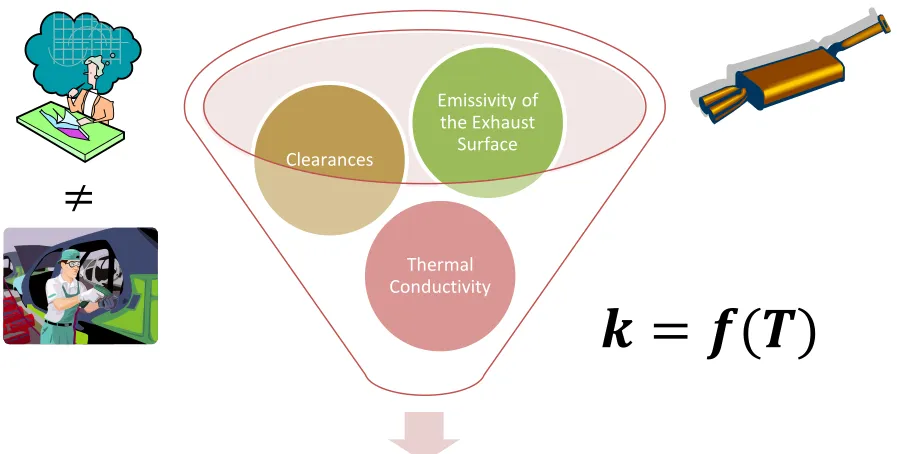
Figure 1 - Many Sources of Uncertainty Exist for the Thermal Performance of
Underbody Components Resulting in an Unpredictable Thermal System
On a number of vehicle architectures, the spare tire tub is an underbody component
which is directly above the muffler and therefore can be strongly affected by the variation
UNPREDICTABLE THERMAL SYSTEM
ThermalConductivity Clearances
Emissivity of the Exhaust
Surface
≠
19
in the emissivity of the exhaust surface. This underbody component has significant
interest to the aero/thermal organization and was therefore selected as a case study for the
application of the FAST method coupled with DFSS.
CHAPTER 4
APPLICATION OF THE FOURIER AMPLITUDE SENSITIVITY
TEST (FAST) METHOD TO AN UNDERBODY COMPONENT
Fourier Amplitude Sensitivity Test (FAST)
For this case study, the FAST method was used to investigate the effect of uncertainty in
design parameters on thermal system performance of the spare tire tub. The results from
this study will pinpoint the design parameters which offer the greatest opportunity for
improvement of thermal system performance and reliability. In turn, this method can save
engineering time and resources.
The first step required to apply the FAST method is to form an analytical model for the
system to be studied. For this case study, the vehicle underbody system consists of a
muffler, a three-layer heat shield, and spare tire tub. The output of interest from this
model is the temperature of the spare tire tub. The majority of the input parameters in this
model deviate from their nominal values due to environmental factors, wear and ageing,
and/or variation in the manufacturing process. Using MATLAB software package, the
model was simulated with input parameters which were simultaneously and sinusoidally
varied at distinct frequencies over their respective uncertainty ranges.
Finally, the Fourier transform was applied to the output of the model to convert the
20
frequencies to be recognized. The amplitude of each frequency was used as an indication
of the strength of the effect of the corresponding parameter’s variation on the temperature
of the spare tire tub. Reducing the partial variance of the most influential input
parameters by decreasing the system’s sensitivity to these parameters and/or decreasing
the uncertainty of these parameters will have the greatest improvement on the overall
thermal performance of the system.
Analytical Model Development
The analytical model is developed to represent the thermal system containing the
underbody component of interest. For this case study, the component of interest is the
spare tire tub. A configuration in which this component is located directly above the
muffler was considered. In vehicles with this particular configuration, there is usually a
heat shield located between the muffler and the underbody component to protect the
component from the radiation energy emitted by the muffler. This model considered the
heat shield to consist of three layers; two aluminum layers with a layer of fiberglass in
21
The components within this system exchange heat by three modes; conduction,
convection, and radiation.
Figure 2 - Sketch of Underbody Components Considered in the Analytical Model
Energy Balance Equations
The following section explains the steps followed to develop the analytical model. To
begin, the definition of the parameters used within the model are presented in Table 1.
The fifth column in this table provides the nominal values approximated for each of these
parameters. A brief description of the determination of these values is shown in the
22
Table 1 - Input Parameters for the Analytical Model Developed to Implement the FAST
Method
No. Parameter Component(s) Matlab Definition
Nominal
Value Unit Uncertainty
1
Convection Heat Transfer
Coefficients
Air to Spare Tire Tub ℎ𝑠𝑡 10 W/(m^2 K) -31.0% 31.0%
2 Air to Heat Shield Lower Surface
ℎℎ𝑠𝑙 13 W/(m^2 K) -76.0% 76.0%
3 Air to Heat Shield Upper
Surface ℎℎ𝑠𝑢
7 W/(m^2 K) -29.0% 29.0%
4
Temperatures
Muffler Surface 𝑇𝑚 603 K -30.0% 30.0%
5 Air Flow Over Heat Shield
Upper Surface
𝑇𝑎ℎ𝑠𝑢
320 K -20.0% 20.0%
6 Air Flow Over Heat Shield
Lower Surface
𝑇𝑎ℎ𝑠𝑙
333 K -20.0% 20.0%
7 Air Flow Over Spare Tire
Tub
𝑇𝑎𝑠𝑡 317 K -20.0% 20.0%
8
Emissivities
Muffler 𝜀𝑚 0.2 - 0.0% 350.0%
9 Spare Tire Tub 𝜀𝑠𝑡 0.9 - 0.0% 0.0%
10 Heat Shield 𝜀ℎ𝑠 0.45 - 0.0% 100.0%
11
Densities
Spare Tire Tub 𝜌𝑠𝑡 7769 kg/m^3 -10.0% 10.0%
12 Heat Shield (Outer Layer) 𝜌ℎ𝑠_𝑜 2770 kg/m^3 -10.0% 10.0%
13
Specific Heat Capacities
Spare Tire Tub 𝑐𝑠𝑡 461 J/(kg K) -7.0% 7.0%
14 Heat Shield (Outer Layer) 𝑐ℎ𝑠_𝑜 884 J/(kg K) -7.0% 7.0%
15 Thermal Conductivities
Heat Shield (Inner Layer) 𝑘ℎ𝑠_𝑖 0.3 W/(m K) -7.0% 7.0%
16
Thicknesses
Spare Tire Tub 𝑡𝑠𝑡 0.002 m -13.33% 13.33%
17 Heat Shield (Outer Layer) 𝑡ℎ𝑠_𝑜 0.00025 m -78.74% 78.74%
18 Heat Shield (Inner Layer) 𝑡ℎ𝑠_𝑖 0.004 m -5.00% 5.00%
19
Lengths
Spare Tire Tub 𝐿𝑠𝑡 0.456 m -0.044% 0.044%
20 Heat Shield 𝐿ℎ𝑠 0.456 m -0.044% 0.044%
21
Widths
Spare Tire Tub 𝑊𝑠𝑡 0.811 m -0.025% 0.025%
22 Heat Shield 𝑊ℎ𝑠 0.811 m -0.025% 0.025%
23
Diameters
Muffler Diameter 1 𝐷1𝑚 0.180 m -0.111% 0.111%
24 Muffler Diameter 2 𝐷2𝑚 0.230 m -0.087% 0.087%
25
Clearances
Heat Shield to Spare Tire Tub
𝐿ℎ𝑠_𝑠𝑡 0.002 m -10.20% 10.20%
23
To develop the analytical model for this case study, the first law of thermodynamics was
applied. The first law of thermodynamics is also referred to as the principle of
conservation of energy (Cengel & Ghajar, 2014). This law states that energy cannot be
created or destroyed; however, it can change forms. This law can be expressed as the
following.
Equation 18
(𝑇𝑜𝑡𝑎𝑙 𝐸𝑛𝑒𝑟𝑔𝑦 𝐸𝑛𝑡𝑒𝑟𝑖𝑛𝑔 𝑡ℎ𝑒 𝑆𝑦𝑠𝑡𝑒𝑚) − (𝑇𝑜𝑡𝑎𝑙 𝐸𝑛𝑒𝑟𝑔𝑦 𝐿𝑒𝑎𝑣𝑖𝑛𝑔 𝑡ℎ𝑒 𝑆𝑦𝑠𝑡𝑒𝑚)
= (𝐶ℎ𝑎𝑛𝑔𝑒 𝑖𝑛 𝑡ℎ𝑒 𝑇𝑜𝑡𝑎𝑙 𝐸𝑛𝑒𝑟𝑔𝑦 𝑜𝑓 𝑡ℎ𝑒 𝑆𝑦𝑠𝑡𝑒𝑚)
For a general system undergoing any process, this law can be expressed in the following
terms.
Equation 19
𝐸̇𝑖𝑛− 𝐸̇𝑜𝑢𝑡 = ∆𝐸𝑠𝑦𝑠𝑡𝑒𝑚 𝑑𝑡
When the system is not subject to substantial surface tension, gravity, magnetic, or
electric effects, the term on the right side of this equation can be expressed as the change
in internal energy, as written below.
Equation 20
∆𝐸𝑠𝑦𝑠𝑡𝑒𝑚 = ∆𝑈𝑠𝑦𝑠𝑡𝑒𝑚
When conducting heat transfer analysis, the focus is placed on energy transfer due to a
24
and nuclear energies are placed in to one term of heat generation and the first law can be
written as shown below.
Equation 21
𝑄̇𝑖𝑛− 𝑄̇𝑜𝑢𝑡+ 𝐸̇𝑔𝑒𝑛 =∆𝐸𝑡ℎ𝑒𝑟𝑚𝑎𝑙,𝑠𝑦𝑠𝑡𝑒𝑚 𝑑𝑡
In this specific analysis, the components include the muffler, heat shield, and spare tire
tub. These components have a fixed mass; therefore, they are considered to be closed
systems. In this case, the equation can be further simplified, as depicted below.
Equation 22
𝑄̇𝑖𝑛− 𝐸̇𝑜𝑢𝑡 = ∆𝑈̇ = 𝑚𝑐𝑣
𝑑𝑇 𝑑𝑡
One final simplification can be made because there are no work interactions across the
boundaries of the components in this system. Therefore, all of the energy in and out of
the system is transferred by heat. With this understanding, the equation can be written as
below.
Equation 23
𝑄̇𝑖𝑛− 𝑄̇𝑜𝑢𝑡 = 𝑚𝑐𝑣𝑑𝑇 𝑑𝑡
The terms on the left side of this equation represent the net amount of heat transfer across
the boundary of the component. A component may have heat transferred across the
25 Conduction
Conduction can occur in any phase of a substance. This form of heat transfer takes place
when heat is transferred from particles with more energy to particles with less energy. It
depends upon the thermal conductivity of the substance, the dimensions of the substance,
and the temperature difference from one side of the substance to the other. Fourier’s Law
of heat conduction governs this mode of heat transfer and is shown below.
Equation 24
𝑄̇𝑐𝑜𝑛𝑑 = 𝑘𝐴𝑑𝑇 𝑑𝑥
In this analytical model, the heat shield and spare tire tub are modelled as plane walls.
The equation for heat transfer by conduction through a plane wall is shown below.
Equation 25
𝑄̇𝑐𝑜𝑛𝑑 = 𝑘𝐴∆𝑇 ∆𝑥
Where:
𝑘 is the thermal conductivity of the substance
𝐴 is the cross-sectional area of the substance
∆𝑇 is the temperature difference across the thickness of the substance
26 Convection
The second mode of heat transfer to be discussed is convection. This mode of heat
transfer is conduction in the presence of fluid motion. Thus, this form of heat transfer
occurs between a solid and liquid or a solid and gas. This form of heat transfer is
governed by Newton’s Law of cooling, shown below.
Equation 26
𝑄̇𝑐𝑜𝑛𝑣 = ℎ𝐴𝑠(𝑇𝑠− 𝑇∞)
Where:
ℎ is the heat transfer coefficient (determined experimentally)
𝐴𝑠 is the surface area of the solid
𝑇𝑠 is the temperature of the solid surface
𝑇∞ is the temperature of the fluid flowing over the solid surface
Radiation
Radiation is a form of heat transfer which occurs due to variations in the electronic
arrangements of atoms and/or molecules. This form of heat transfer occurs as
electromagnetic waves and does not require a medium. The equation which governs this
form of heat transfer is the Stefan-Boltzmann law, shown below.
Equation 27
27 Where:
𝜀 is the emissivity of the surface
𝜎 is the Stefan-Boltzmann constant (5.67 x 10⁻⁸ 𝑊 𝑚2𝐾4)
𝐴𝑠 is the surface area
𝑇𝑠 is the temperature of the surface
When radiation strikes a surface, the radiation can be absorbed, reflected, and/or
transmitted. The incident radiation, also known as irradiation, G, can be written in the
form shown below.
𝐺 = 𝐺𝑎𝑏𝑠+𝐺𝑟𝑒𝑓+𝐺𝑡𝑟𝑎
The fraction of radiation which is absorbed, reflected, and transmitted depends on the
absorptivity of the surface, 𝛼, the reflectivity of the surface, ρ, and the transmissivity of
the surface, 𝜏.
Equation 28
𝛼 = 𝐺𝑎𝑏𝑠 𝐺
Equation 29
𝜌 = 𝐺𝑟𝑒𝑓 𝐺
Equation 30
28
Substituting these three relationships into Equation 27 results in the following equation.
Equation 31
𝛼 + 𝜌 + 𝜏 = 1
For the three components in this analysis (lower layer of heat shield, upper layer of heat
shield, and spare tire tub), the transmitted radiation is assumed to be negligible because
these surfaces are opaque. Therefore, a portion of the incident radiation is absorbed,
which will increase the thermal energy of the component and another portion is reflected
away from the component.
In the following three sections, Equation 23 will be used to develop an energy balance for
the lower layer of the heat shield, the upper layer of the heat shield, and the component of
interest (the spare tire tub). These energy balances will include conduction, convection,
and radiation terms to describe the energy transfer across the boundaries of these three
components which will result in a change in thermal energy of the components. The
purpose of developing these equations is to identify the design parameters which affect
the temperature of the spare tire tub so that uncertainty analysis can be conducted on
these parameters.
Energy Balance for the Lower Layer of the Heat Shield
The lower layer of the heat shield is modelled as a closed system with no work
interactions; thus, the energy balance for the lower layer of the heat shield can be
29
Equation 32
𝑄̇𝑖𝑛− 𝑄̇𝑜𝑢𝑡 = 𝑚𝑐𝑣𝑑𝑇 𝑑𝑡
The left side of the equation is the net heat transfer to this layer and the right side
provides the corresponding increase in temperature. Therefore, the sources of heat
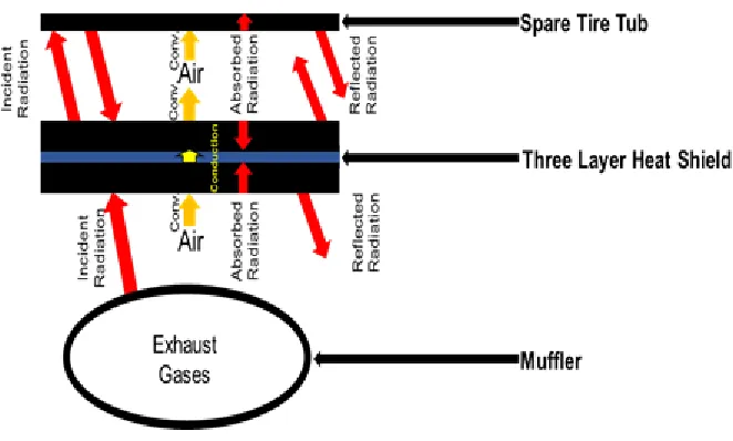
transfer to and away from this component need to be identified. This layer experiences
heat transfer by conduction, convection, and radiation. A diagram which shows these
modes of heat transfer is given below.
Figure 3 - Energy Balance of Lower Layer of Heat Shield
Conduction
Conduction occurs at the upper boundary of this component through the inner layer of the
30
layer of the heat shield and the upper layer of the heat shield. The equation for this
conduction heat transfer, based on Fourier’s Law of heat conduction, is given below.
Equation 33
𝑄̇𝑐𝑜𝑛𝑑 = 𝑘ℎ𝑠𝑖𝐴ℎ𝑠
(𝑇ℎ𝑠𝑢− 𝑇ℎ𝑠𝑙) 𝑡ℎ𝑠𝑖
Convection
Convection occurs at the lower boundary of this component due to the underbody
airflow. The equation, based on Newton’s Law of cooling, is given below.
Equation 34
𝑄̇𝑐𝑜𝑛𝑣= ℎℎ𝑠𝑙𝐴ℎ𝑠(𝑇𝑎ℎ𝑠𝑙 − 𝑇ℎ𝑠𝑙)
Radiation
To simplify the analysis of the radiation heat transfer to this component, the lower layer
of the heat shield was assumed to be gray, opaque, and diffuse. A gray surface is one
whose emissivity is equal to its absorptivity. An opaque surface does not transmit any of
the incident radiation; thus, it is not transparent. A diffuse surface emits and reflects
radiation in a manner which is independent of the wavelength of the radiation and is
isothermal.
The majority of the incident radiation to this component, 𝐺̇, will come from the surface of
the muffler because it is at a highly elevated temperature. The fraction of radiation
emitted by the muffler which actually strikes the heat shield will depend upon the view
factor from the muffler to the heat shield, 𝐹𝑚−ℎ𝑠𝑙. The equation for the incident radiation,
31
Equation 35
𝐺̇ = 𝜀𝑚𝜎𝐴𝑚𝐹𝑚−ℎ𝑠𝑙𝑇𝑚4
The calculation of the view factor from a cylinder to a plane wall is more complex than
the view factor from a plane wall to a cylinder. To reduce the complexity of the view
factor calculation, the reciprocity relation was applied. This relation is show below.
Equation 36
𝐴𝑖𝐹𝑖−𝑗 = 𝐴𝑗𝐹𝑗−𝑖
Applying the reciprocity relation to the muffler and lower surface of the heat shield
renders the following.
Equation 37
𝐴𝑚𝐹𝑚−ℎ𝑠𝑙 = 𝐴ℎ𝑠𝐹ℎ𝑠𝑙−𝑚
Thus, to simplify the calculations, the irradiation was expressed by the equation below.
Equation 38
𝐺̇ = 𝜀𝑚𝜎𝐴𝑚𝐹𝑚−ℎ𝑠𝑙𝑇𝑚4 = 𝜀𝑚𝜎𝐴ℎ𝑠𝐹ℎ𝑠𝑙−𝑚𝑇𝑚4
A portion of this irradiation will be reflected away from the heat shield and the rest will
be absorbed, increasing the thermal energy of the component. The amount of reflected
radiation depends on the reflectivity of the surface, 𝜌, as shown in the equation below.
Equation 39
𝐺̇𝑟𝑒𝑓= 𝜌𝐺̇ = 𝜌ℎ𝑠𝑙𝜀𝑚𝜎𝐴ℎ𝑠𝐹ℎ𝑠𝑙−𝑚𝑇𝑚4
Since this surface was assumed to be gray (𝜀 = 𝛼) and opaque (𝜏 = 0), the reflected
32
Equation 40
𝐺̇𝑟𝑒𝑓= 𝜌𝐺̇ = (1 − 𝜀ℎ𝑠𝑙)𝜀𝑚𝜎𝐴ℎ𝑠𝐹ℎ𝑠𝑙−𝑚𝑇𝑚4
The amount of radiation which is absorbed can also be expressed as the difference
between the amount of incident radiation and the amount of reflected radiation.
Equation 41
𝐺̇𝑎𝑏𝑠 = 𝐺̇ − 𝐺̇𝑟𝑒𝑓 = 𝜀𝑚𝜎𝐴ℎ𝑠𝐹ℎ𝑠𝑙−𝑚𝑇𝑚4− (1 − 𝜀ℎ𝑠𝑙)𝜀𝑚𝜎𝐴ℎ𝑠𝐹ℎ𝑠𝑙−𝑚𝑇𝑚4
Radiation will also be emitted from the lower layer of the heat shield’s surface to the
surroundings.
Equation 42
𝑄̇𝑟𝑎𝑑 𝑒𝑚𝑖𝑡 = 𝜀ℎ𝑠𝜎𝐴ℎ𝑠𝑇ℎ𝑠𝑙4
Substituting the conduction, convection, and radiation terms into the energy balance,
Equation 32, yields the following.
Equation 43
𝑚ℎ𝑠𝑙𝑐ℎ𝑠𝑑𝑇ℎ𝑠𝑙
𝑑𝑡 = 𝑄̇𝑐𝑜𝑛𝑑 + 𝑄̇𝑐𝑜𝑛𝑣+ 𝐺̇𝑎𝑏𝑠− 𝑄̇𝑟𝑎𝑑 𝑒𝑚𝑖𝑡
Substituting the equations for convection, conduction, radiation emitted, and radiation
33
Equation 44
𝑚ℎ𝑠𝑙𝑐ℎ𝑠_𝑜𝑑𝑇ℎ𝑠𝑙 𝑑𝑡
= 𝑘ℎ𝑠𝑖𝐴ℎ𝑠
(𝑇ℎ𝑠𝑢 − 𝑇ℎ𝑠𝑙) 𝑡ℎ𝑠𝑖
+ ℎℎ𝑠𝑙𝐴ℎ𝑠(𝑇𝑎ℎ𝑠𝑙 − 𝑇ℎ𝑠𝑙) + 𝜀𝑚𝜎𝐴ℎ𝑠𝐹ℎ𝑠𝑙−𝑚𝑇𝑚
4
− (1 − 𝜀ℎ𝑠𝑙)𝜀𝑚𝜎𝐴ℎ𝑠𝐹ℎ𝑠𝑙−𝑚𝑇𝑚4 + 𝜀ℎ𝑠𝑙𝜎𝐴ℎ𝑠𝑇ℎ𝑠𝑙4
In this form of the equation, there are parameters which are dependent on one another.
These parameters are the view factor from the lower layer of the heat shield to the muffler,
the surface area of the heat shield, and the mass of the heat shield. These interactions are
not ideal for DFSS analysis. Therefore, the view factor, surface area, and mass terms were
substituted with equations which are functions of the geometric properties of the system.
The view factor from the heat shield to the muffler was found by approximating the muffler
as an infinitely long cylinder and the heat shield as an infinitely long flat plate. The formula
for this view factor was found from the ASME paper, “Compilation of Radiation Shape
Factors for Cylindrical Assemblies” (Leuenberger & Person, 1994).
Equation 45
𝐹2→1 = 2𝑅 𝑇 𝑡𝑎𝑛
−1 𝑇
2𝑆
Where:
2 is the flat plate
1 is the cylinder
34
𝑇 is the length of the plate
𝑆 is the distance between the cylinder axis and the plate
Substituting the variables being used in this model, the formula for the view factor from
the heat shield to the muffler becomes:
Equation 46
𝐹ℎ𝑠𝑙−𝑚 = 2(𝐷1𝑚 + 𝐷2𝑚) 4𝐿ℎ𝑠 𝑡𝑎𝑛
−1 𝐿ℎ𝑠
2𝐿𝑚_ℎ𝑠
The surface area of the lower surface of the heat shield was put in to terms of the
dimensions of the heat shield by approximating it as a flat plate; thus, the surface area was
simply calculated by multiplying the length and width. The mass of the lower layer of the
heat shield was calculated by multiplying the density of the lower layer of the heat shield
by the volume. The volume was calculated as the product of length, width, and thickness.
Therefore, the final energy balance equation for the lower layer of the heat shield was
formed.
Equation 47
𝜌ℎ𝑠_𝑜𝐿ℎ𝑠𝑊ℎ𝑠𝑡ℎ𝑠_𝑜𝑐ℎ𝑠_𝑜𝑑𝑇ℎ𝑠𝑙 𝑑𝑡
= 𝑘ℎ𝑠_𝑖(𝐿ℎ𝑠𝑊ℎ𝑠)(𝑇ℎ𝑠𝑢 − 𝑇ℎ𝑠𝑙)
𝑡ℎ𝑠_𝑖 + ℎℎ𝑠𝑙(𝐿ℎ𝑠𝑊ℎ𝑠)(𝑇𝑎ℎ𝑠𝑙 − 𝑇ℎ𝑠𝑙)
+ 𝜀𝑚𝜎(𝐿ℎ𝑠𝑊ℎ𝑠)(2(𝐷1𝑚 + 𝐷2𝑚)
4𝐿ℎ𝑠 𝑡𝑎𝑛
−1 𝐿ℎ𝑠
2𝐿𝑚_ℎ𝑠)𝑇𝑚
4− (1
− 𝜀ℎ𝑠)𝜀𝑚𝜎(𝐿ℎ𝑠𝑊ℎ𝑠)(2(𝐷1𝑚 + 𝐷2𝑚) 4𝐿ℎ𝑠 𝑡𝑎𝑛
−1 𝐿ℎ𝑠
2𝐿𝑚_ℎ𝑠)𝑇𝑚
4
35
Energy Balance for the Upper Layer of the Heat Shield
The same method used for the lower surface of the heat shield was used to develop the
energy balance equation for the upper surface of the heat shield. To begin, the general
form of the energy balance equation for a closed system with no work interactions was
applied.
Equation 48
𝑄𝑖𝑛̇ − 𝑄𝑜𝑢𝑡̇ = 𝑚𝑐𝑣
𝑑𝑇 𝑑𝑡
To determine the net heat transfer to this component, the modes of heat transfer were
identified as shown in the figure below.
36 Conduction
Conduction occurs at the lower boundary of this component through the inner layer of the
heat shield. This heat transfer is driven by the temperature difference between the lower
layer of the heat shield and the upper layer of the heat shield. The equation for this
conduction heat transfer, based on Fourier’s Law of heat conduction, is given below.
Equation 49
𝑄̇𝑐𝑜𝑛𝑑 = 𝑘ℎ𝑠𝑖𝐴ℎ𝑠
(𝑇ℎ𝑠𝑙− 𝑇ℎ𝑠𝑢) 𝑡ℎ𝑠𝑖
Convection
Convection occurs at the upper boundary of this component due to the underbody
airflow. The equation, based on Newton’s Law of cooling, is shown here.
Equation 50
𝑄̇𝑐𝑜𝑛𝑣 = ℎℎ𝑠𝑢𝐴ℎ𝑠(𝑇𝑎ℎ𝑠𝑢− 𝑇ℎ𝑠𝑢)
Radiation
As discussed during the development of the energy balance for the lower layer of the heat
shield, the analysis was simplified by assuming that the upper layer of the heat shield is
gray, opaque, and diffuse.
The incident radiation to the upper layer of the heat shield, 𝐺̇, will come from the surface
of the spare tire tub. The fraction of radiation emitted by the spare tire tub which strikes
the heat shield will depend upon the view factor from the spare tire tub to the upper
surface of the heat shield, 𝐹𝑠𝑡−ℎ𝑠𝑢. The equation for the incident radiation, based on the
37
Equation 51
𝐺̇ = 𝜀𝑠𝑡𝜎𝐴𝑠𝑡𝐹𝑠𝑡−ℎ𝑠𝑢𝑇𝑠𝑡4
A portion of this irradiation will be reflected away from the heat shield and the rest will
be absorbed, increasing the thermal energy of the component. The amount of reflected
radiation depends on the reflectivity of the surface, 𝜌, as shown in the equation below.
Equation 52
𝐺̇𝑟𝑒𝑓 = 𝜌𝐺̇ = 𝜌ℎ𝑠𝑢𝜀𝑠𝑡𝜎𝐴𝑠𝑡𝐹𝑠𝑡−ℎ𝑠𝑢𝑇𝑠𝑡4
Since this surface was assumed to be gray (𝜀 = 𝛼) and opaque (𝜏 = 0), the reflected
radiation can also be expressed by the following equation.
Equation 53
𝐺̇𝑟𝑒𝑓 = 𝜌𝐺̇ = (1 − 𝜀ℎ𝑠)𝜀𝑠𝑡𝜎𝐴𝑠𝑡𝐹𝑠𝑡−ℎ𝑠𝑢𝑇𝑠𝑡4
The amount of radiation which is absorbed can also be expressed as the difference
between the amount of incident radiation and the amount of reflected radiation.
Equation 54
𝐺̇𝑎𝑏𝑠 = 𝐺̇ − 𝐺̇𝑟𝑒𝑓= 𝜀𝑠𝑡𝜎𝐴𝑠𝑡𝐹𝑠𝑡−ℎ𝑠𝑢𝑇𝑠𝑡4− (1 − 𝜀ℎ𝑠)𝜀𝑠𝑡𝜎𝐴𝑠𝑡𝐹𝑠𝑡−ℎ𝑠𝑢𝑇𝑠𝑡4
Radiation will also be emitted from the upper layer of the heat shield’s surface to the
surroundings.
Equation 55
38
Substituting the conduction, convection, and radiation terms into the energy balance,
Equation 48, yields the following.
Equation 56
𝑚ℎ𝑠𝑢𝑐ℎ𝑠𝑑𝑇ℎ𝑠𝑢
𝑑𝑡 = 𝑄̇𝑐𝑜𝑛𝑑+ 𝑄̇𝑐𝑜𝑛𝑣+ 𝐺̇𝑎𝑏𝑠− 𝑄̇𝑟𝑎𝑑 𝑒𝑚𝑖𝑡
Substituting the equations for convection, conduction, radiation emitted, and radiation
absorbed provides the equation below.
Equation 57
𝑚ℎ𝑠𝑐ℎ𝑠_𝑜
𝑑𝑇ℎ𝑠𝑢 𝑑𝑡
= 𝑘ℎ𝑠𝑖𝐴ℎ𝑠(𝑇ℎ𝑠𝑙− 𝑇ℎ𝑠𝑢)
𝑡ℎ𝑠𝑖 + ℎℎ𝑠𝑢𝐴ℎ𝑠(𝑇𝑎ℎ𝑠𝑢− 𝑇ℎ𝑠𝑢) + 𝜀𝑠𝑡𝜎𝐴𝑠𝑡𝐹𝑠𝑡−ℎ𝑠𝑢𝑇𝑠𝑡
4
− (1 − 𝜀ℎ𝑠)𝜀𝑠𝑡𝜎𝐴𝑠𝑡𝐹𝑠𝑡−ℎ𝑠𝑢𝑇𝑠𝑡4− 𝜀ℎ𝑠𝜎𝐴ℎ𝑠𝑇ℎ𝑠𝑢4
As described in the previous section, the view factors, surface areas, and masses were
written in terms of dimensional properties to avoid using parameters which depend on
one another. The equation for the view factor from the spare tire tub to the upper surface
of the heat shield was found by approximating the heat shield and spare tire tub as
parallel flat plates of the same dimensions. The formula for this configuration was found
from the textbook, “Heat and Mass Transfer: Fundamentals and Applications” (Cengel &