and its Analysis
Sanjay Bhattacherjee Applied Statistics Unit Indian Statistical Institute
203, B.T.Road, Kolkata, India - 700108. sanjayb [email protected]
Palash Sarkar Applied Statistics Unit Indian Statistical Institute
203, B.T.Road, Kolkata, India - 700108. [email protected]
Abstract
The Subset Difference (SD) method proposed by Naor-Naor-Lotspeich is the most popular broadcast en-cryption (BE) scheme. It is suitable for real-time applications like Pay-TV. It has been suggested for use by the AACS standard for digital rights management in Blu-Ray and DVD discs. The SD method assumes the number of users to be a power of two. (1) We propose the Complete Tree Subset Difference (CSD) method that subsumes the SD method by allowing arbitrary number of users in the system. All the results obtained in this work for the CSD scheme hold good for the SD scheme by assuming the number of users to be the next power of two. (2) Given the importance of the SD scheme, its detailed combinatorial analysis is of practical interest. We find recurrences for the CSD scheme to count the number of possible waysrusers in the system ofnusers can be revoked to result in a transmission overhead (header length) ofh. The header lengthhof a broadcast is an important efficiency parameter in BE. The usefulness of these recurrences is demonstrated by generating exhaustive data of the above count, obtaining bounds on the header length and various other interesting results some of which are difficult to prove without the recurrences. (3) AnO(rlogn) time algorithm is proposed to compute the expected header length in the CSD scheme fornusers in the system,rout of which are revoked. This algorithm is of practical interest in its own right, for efficiency and performance analysis of the CSD scheme. Using this algorithm, we show that for practical values of nandr, the transmission efficiency of the CSD scheme is better than the SD scheme. Forna power of two and a fixedr≥2, we obtain an upper bound on the expected header length and show that this bound is also the limit asn→ ∞.
1
Introduction
1.1 What is Broadcast Encryption?
The cryptographic method for a centre to efficiently broadcast encrypted digital content to a system of users so that only an intended subset (theprivileged users) can correctly decrypt it is calledBroadcast Encryption (BE). Before the system starts to work, the users are given some secret information (may be the secret keys or some information from which it can derive the secret keys). A user uses this information for decrypting the encrypted digital content intended for itself.
In a typical BE scheme, each message (a block of digital content) that is broadcast is encrypted using a unique key called a session key. The session key in turn, is encrypted a number of times using user keys and these multiple encryptions of the session key is sent as the header of the encrypted message. The transmission overhead of the scheme is determined by the header length h (the number of encryptions of the session key in the header).
In a fully resilient scheme, even if an adversary has the decryption keys of all the remaining non-privileged users in the system (therevoked users), it will not be able to correctly decrypt the content. A crucial requirement
for a BE scheme is that it should facilitate dynamic revocation of decryption privilege from any subset of users at any point of time (based on their subscription or privilege status).
Importance of Broadcast Encryption: Copyright protection using Digital Rights Management [DRM] techniques is an important application of BE. Out of the different facets of copyright protection, BE handles the content protection part. The application of BE systems is pretty wide in the implementation of [DRM] for content protection in digital data distribution technologies such as pay-TV, Internet or mobile video broadcast, optical discs, etcetera.
Requirements from a BE scheme: In real-time scenarios like Pay-TV, Internet or mobile video broadcast, the number of users can vary from a few thousands to millions. For other real-time applications of BE like broadcasting secret instructions to military outposts from a base station, the number of users will be much smaller (maximum of a few hundreds). The BE scheme that is used in real time scenarios as above, has to be efficient in terms of the transmission overhead associated with each message as also the encryption and decryption times and storage of user keys.
For non-real-time applications like content protection in Blu-Ray discs and DVDs (optical discs), the require-ments from a BE scheme are somewhat different. The number of users (disc players) in such scenarios maybe in millions. The transmission overhead (the additional information stored in the physical media, that is used for decrypting the content) is not really an issue since storage space in discs is no more a constraint nowadays. Further, since encryption does not happen in real-time, improving the encryption time is also not very important. On the other hand, reducing the user storage (number of keys or their equivalent secret to be stored in the player) and decryption time is still important.
Importance of the [NNL01] SD scheme: Broadcast Encryption was introduced in [Ber91] followed by [FN93]. There have been several works in this area [Sti97], [SW98] since then, but the most popular scheme out of these is the tree-based Subset Difference (SD) method of [NNL01]. Since it is a symmetric key based scheme, it is very efficient in terms of encryption and decryption time. It allows the users to be stateless (users do not have to update their individual secret information with every session) and also allows dynamic revocation of users. User storage requirement isO(log2n) wherenis the total number of users and the transmission overhead is linear in the number of revoked users r. Currently, the SD scheme offers the simplest algorithm and the best trade-offs for use in both real-time applications like Pay-TV and non-real time applications like content protection in optical discs [AAC].
1.2 Our Contributions:
Arbitrary number of users: In this paper, we broaden the scope of use of the SD scheme. The SD scheme and all follow-up works [HS02, PB06, AK08, MMW09] assume the total number of users n to be a power of two. We relax this restriction to allow any arbitrary number of users in the system by introducing the Complete Tree Subset Difference (CSD) scheme. The CSD scheme is based on the SD scheme and subsumes it. When the number of users in the CSD method is a power of two, it becomes exactly the same as the SD scheme.
Inclusion of dummy users results in the expected header length of the SD scheme to be more than the CSD scheme for practical values ofnandr. This is intuitive and we provide further arguments and supporting data in Section 3.2 and Section 5.4. In real-time scenarios like Pay-TV, where many messages are transmitted, avoiding the extra bandwidth arising due to dummy users will be desirable. Consequently, one would prefer to exclude them and instead work with the actual number of users present in the system.
It is to be noted that an implementation that uses the SD scheme, can easily shift to using the CSD scheme with minimal change in the software implementation. This is because the internal tree structure used for assigning keys to subsets of users in the SD scheme remains almost the same in the CSD scheme.
Combinatorial Analysis: The importance of the (C)SD scheme motivates the study of its combinatorial properties. We use a new approach for a detailed combinatorial study of the CSD scheme. A method is proposed to count the number of ways thatr out ofnusers can be revoked to get a header length ofhin the CSD scheme. This counting is formulated using two recurrences. Since the SD scheme is a special case of the CSD scheme, these recurrences hold for the SD scheme too.
Using these recurrences, a dynamic programming based algorithm to do the above counting is developed. Previous to this work, the only known method to do such counting was to run the SD algorithm itself on all possible nrrevocation patterns. The resulting time complexity can be exponential inn. In contrast, the running time of the algorithm proposed here is always polynomial inn. This, by itself, is a significant improvement.
The importance of these recurrences in capturing the detailed combinatorial properties of the CSD scheme is demonstrated by obtaining important results from them.
1. The worst case header length for a given r in the SD scheme was shown to be 2r−1 in [NNL01]. We show that the worst case header length for the CSD scheme is min(2r−1,dn/2e, n−r).
2. Given r, we characterize the minimum number of users nr (that need to be in a system using the CSD method), that can give rise to the maximum header length of 2r−1.
3. For the special case when nis a power of two (i.e., for the SD scheme), we use the recurrences to obtain a generating function for the sequence. Earlier, a generating function of a slightly different form was obtained in [PB06] using direct arguments. We did not attempt to find the generating function for the case when n
is not a power of two. This would be quite cumbersome and did not appear to be of much interest.
Probabilistic analysis: We propose a new and efficient O(rlogn) algorithm for computing the expected header length in the CSD method for a given n and r. This algorithm is based on the probabilistic analysis of revocation of users. It is simple to implement. The crucial importance of the algorithm lies in the fact that it enables us to explore in depth the behaviour of the expected header length for values of n ranging from a few hundreds to a million. Examples of outputs obtained by running the algorithm are provided later. We believe that the algorithm for computing the expected header length will be a very useful tool for practitioners implementing the (C)SD scheme.
Whennis a power of two (i.e., the SD scheme), we show that the expected header length forr revoked users is bounded above by
(3r−2)−3× r−1
X
i=1
−1 2
i
+ i
X
k=1 (−1)k
i k
(2k−3k) (2k−1)
!
.
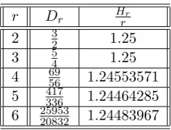
We further show that asn→ ∞through powers of two, this is actually the limiting value of the expected header length. Computing the above expression for different values ofr shows it to be always less than 1.25r.
1.25r. Our analysis of the expected header length shows the precise limiting upper bound and clarifies the issue of this value being 1.25r.
1.3 Previous and related works:
The tree-based SD scheme has inspired quite a lot of work in the area of broadcast encryption. Asymptotic improvements to the user storage parameter of the SD scheme were suggested in the tree-based LSD scheme of [HS02] with some loss of efficiency in the transmission overhead. Analysis of the combinatorics behind broadcast encryption schemes and different generic bounds on the efficiency parameters have been done in [LS98, PGM04] and other works. A generic method for constructing BE schemes from pseudo-random generators was proposed in [AKI03].
An analysis of the expected header length of the SD and LSD schemes was done in [PB06]. As mentioned earlier, they proposed generating functions for counting the number of wayspusers (out of totalnusers) can be given access privilege so that the header length will be h. Using this generating function, they found equations to compute the expected header length for a given nand r. However, they admitted that their equations were “complex to compute and difficult to gain insight from”. Consequently they went forward to findapproximations
for the same. The analysis of the expected header length in [PB06] was continued in [EOPR] to show that the standard deviations are small compared to the means as the number of users gets large. Other combinatorial studies of the SD method has been done in [MMW09, AK08]. In particular, the maximum possible header length for a given nand r was found accurately in [MMW09].
Extension of [BS11]: This work is the extended and considerably modified version of [BS11]. The work in [BS11] was the first to propose accommodating arbitrary number of users by modifying the SD method (that uses afull tree) to use anincomplete tree with the users as its leaves. In the current work, considerable changes have been made in the structure of the tree underlying the scheme. This constitutes the main difference between the current work and that in [BS11]. Although the capability of accommodating arbitrary number of users has been retained, a balanced complete tree structure has been used for assignment of keys to subsets (in place of the unbalanced incomplete tree used in [BS11]). Recurrences to analyze the CSD method has been found in a manner similar to the one found in [BS11]. The algorithm to compute the expected header length in [BS11] has been modified to obtain a similar algorithm for the CSD method of this paper. In Appendix A, we very briefly describe the results of [BS11].
Other related work: There are several other BE schemes. A family of broadcast encryption schemes using linear algebraic techniques and hence called linear broadcast encryption schemes was introduced in [PGMM03]. The same authors had also proposed key pre-distribution techniques based on linear algebraic techniques in [PGMM02]. Another interesting work on BE is [JHC+05]. It works on the idea of “one key per punctured interval” in which the worst case header length has been brought down to r (or below at the cost of increasing user storage) for the first time. But, the method is more complicated than the SD scheme and the user storage requirement is rather high.
Traitor tracing is a related issue. We do not discuss this here, since it is not connected to the contribution of the paper. We only remark that the traitor tracing method for the SD scheme can be modified to obtain a traitor tracing method for the CSD scheme. There are several schemes on public-key BE which we do not consider at all.
2
The Subset Cover Revocation Framework
method that falls under the Subset Cover Revocation Framework that was proposed in the same paper. We begin with a very short description of this framework.
The Subset Cover Revocation Framework assumes acentre that encrypts a messageM and broadcasts it to a setN of (|N |=)nusers. This set of users are all the possible recipients of the broadcast. A subset R(⊆ N) of these users are revoked (say non-subscribers of a service). The centre broadcasts using a broadcast encryption algorithm such that any user belonging to the setN \ Rshould be able to correctly decrypt the messageM from the broadcast, while any coalition of users belonging to the setRshould not be able to correctly decrypt it.
A broadcast encryption algorithm under this framework consists of three parts: (1) an initiation scheme -that assigns user u ∈ N secret information Iu that will allow them to decrypt messages intended for them; (2)
the broadcast algorithm - that takes as input the message M and the set R of revoked users and outputs the ciphertext C. C is broadcast to all the users in N; (3) the decryption algorithm - that runs at the user end. It takes as input the ciphertext C and the secret informationIu that the user uhad received during initiation and attempts to decrypt C. A privileged user should be able to get back the original message M, while a revoked user should not be able to get back the correct message from C.
During initiation, an algorithm in the framework defines a collectionS={S1, . . . ,Sw} of subsets, where each Sj ⊆ N. Each subsetSj is assigned a long-lived keyLj. This assignment may not be explicit as we will see in the Complete Tree Subset Difference algorithm. However, a user u ∈ Sj should be able to deduce Lj from the secret information Iu it had acquired during initiation. During broadcast, given a set R of revoked users, the set of privileged users N \ Ris partitioned into pairwise disjoint subsetsSi1, . . . ,Sihtaken from the collection S. This partition is called the subset cover Sc. In other words,
N \ R= h
[
j=1 Sij
where each Sij ∈ S and Sc={Si1, . . . ,Sih}. The size h of the subset cover is called the header length (we will soon see why).
During broadcast, an algorithm in the framework uses two encryption schemes:
• A function FK : {0,1}∗ → {0,1}∗ to encrypt the message M with a session key K. The session key is a random string chosen afresh for each new messageM.
• A function ELj :{0,1}
∗ → {0,1}∗ to encrypt the session key K with a long-lived keyL
j corresponding to the subsetSj (∈ Sc) of users.
During decryption, a useru has to identify from the header, the set Sij to which it belongs. It decrypts the session key K from the portion of the header that has K encrypted for Sij using the long-lived key Lij that it derives from the secret informationIu it had acquired during initiation. UsingK, it can decrypt the messageM from FK(M). In case the user does not belong to any of the sets in Sc (it is a revoked user), it will not be able to decrypt K orM for that matter.
3
The Complete Tree Subset Difference Method
The Subset Difference (SD) method of [NNL01] and all follow-up work assumes the number of usersn to be a power of two. We propose the Complete Tree Subset Difference (CSD) algorithm that can accommodate any arbitrary number of users.
1 2
6
10
7 14
5 4
3
0
15 16 17 18 19 20 21 22 23 24
11 12 13
9 8
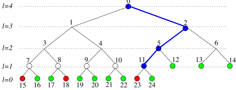
Figure 1: Thecomplete (non-full) treeT0 withn= 13 users as its leaves. Privileged users are indicated in green and the revoked users are indicated in red. Here, r = 3. The tree T1 is a subtree of T0 and is a full subtree having 8 leaf nodes whereas the tree T2 is a non-full complete subtree ofT0 with 5 leaf nodes.
Our algorithm considers a rooted complete binary treeT0 withnleaves. (One may note here that acomplete
binary tree has leaf nodes only at the bottom-most (last) level and maybe also the last-but-one level. The leaves in the last level are filled from the left to the right in the tree. In afull binary tree of height`there are 2`leaves, all at the last level. A full binary tree is also complete by definition. We will refer to trees that are complete but not full asnon-full.) Each user inN is associated with a leaf of the complete binary tree T0. There are 2n−1 nodes (internal and leaf) in T0. These nodes are labeled with numbers from {0,1, . . . ,2n−2}. The root node of T0 is labeled as 0. All subsequent nodes are labeled as follows: the left child node of a nodei is labeled as 2i+ 1 and the right child is labeled as 2i+ 2. Hence, the nodes 0 to n−2 are the internal nodes. The nodes labeled n−1 to 2n−2 are the leaf nodes. The subtree ofT0 rooted at nodeiis denoted byTi. The number of leaf nodes in the subtreeTi is denoted byλi.
Now that we have attached the users to the treeT0, we need to define the collection S of subsets. We define
6
8 9 10
7 12 13 14
5 4
3
0
15 16 17 18 19 20 21 22 23 24
1 2
11
Figure 2: The subset difference subset S1,7 which includes leaves in T1 but not in T7 i.e.; S1,7 = T1\ T7 = {17,18,19,20,21,22}.
During broadcast, the centre will know the setRof revoked users and the messageM to be broadcast. It has to find the subset coverScforN \ R. Scis a collection of pairwise disjoint setsSi1,j1, . . . , Sih,jh (eachSik,jk taken from S) such thatSc =Sh
k=1Sik,jk. If there are no revoked users (R is empty), then the only set in the cover
Sc is N. Otherwise, the following cover-finding algorithm is used: The centre first constructs the Steiner Tree ST(R) induced byRonT0. (The Steiner TreeST(R) is a subgraph ofT0that only retains the nodes and edges on paths from the root node 0 to a revoked leaf node. All the other paths in T0 are deleted.) The cover-finding algorithm runs iteratively by maintaining a tree T that is a sub-graph of ST(R). It starts by initializing T as a copy ofST(R). At every iteration, the algorithm keeps removing nodes from T (while adding subsets to Sc) until T has just one node left. At any point of time in the algorithm, a leaf node in T corresponds to either a leaf node inT0 or the root of a subtree inT0all whose leaves have already been covered till that iteration. More precisely:
1. If there is only one leaf node in T, jump to step 6.
2. Find two leaves j1 and j2 of T whose common ancestor i(both j1 and j2 belong to the minimal subtree Ti) does not have any other leaf node in its subtree inT. (Here, out of the many possible such pairsj
1 and
j2 one may choose the leftmost to have a specific algorithm. Any other choice would have worked equally well.)
3. Let i1 (respectively i2) be the immediate child node of i which is an ancestor of j1 (respectively j2) or is the node j1 (respectively j2) itself. If i1 6=j1 then add the set Si1,j1 to the cover Sc. Similarly, if i2 6= j2
then add the set Si2,j2 to the coverSc.
4. Delete the paths joining j1 and j2 with their common ancestor i.
5. If there are more than one leaf remaining in T, go back to step 2.
6. If the only leaf node is the node 0 (node corresponding to the root of T0), then there are no more subsets to be added to Sc. Else, add the setS0,j (where j is the leaf node remaining inT) to Sc.
3.1 Key assignment to each subset Si,j in S
G. The pseudo-random generatorGoutputs a pseudo-random string that has three times the length of the input seed. The output string G(seed) is divided into three equal parts GL(seed), GM(seed) and GR(seed). (Hence,
G(seed) =GL(seed) kGM(seed)kGR(seed).) G:{0,1}k→ {0,1}3k is a pseudo-random sequence generator if no polynomial time adversary can distinguish between its output for a random seed with a truly random string of the same length.
Seed assignment to nodes: Every non-leaf nodeiinT0 is assigned a uniform random seedLABELi. Every non-root node j of T0 is assigned derived seeds from every ancestor i of j. The left child 2i+ 1 of node i in T0 derives the seed G
L(LABELi) from the random seed LABELi of i. All descendants of 2i+ 1 further get derived seeds from this derived seed GL(LABELi) of 2i+ 1. Similarly, the right child 2i+ 2 of node i in T0 derives the seed GR(LABELi) from the random seed of iand all descendants of 2i+ 2 get derived seeds from this derived seed GR(LABELi) of 2i+ 2. We denote the seed for a node j (that is a descendant ofi) derived from the random seed of node i asLABELi,j. Following such an assignment of random and derived seeds for nodes inT0, the long lived key L
i,j assigned to the setSi,j is GM(LABELi,j).
Iu for each u∈ N: Once the centre is done with the assignment of seeds (uniform random as well as derived) to nodes, it has to distribute the secret information Iu to each useru ∈ N. The user associated with a leafj of T0 must have been revoked when a set S
i,j is in the cover Sc. Hence, the user at leaf j should not be able to compute the Li,j for any of its predecessor iin T0. In fact, it should not be able to compute any Li,k wherek is also one of its ancestors (kmust be a descendant of ithough). In other words, a user at leafj should be able to compute an Li,k if and only if iis an ancestor of j butk is not (k is not on the path joining the leaf j with
i). In a subtree Ti of T0 to which a user at leaf j belongs, the node i has a random seedLABEL
i. The user atj gets the seeds of all nodes adjacent to the path joiningi and j that have been derived fromLABELi. Say
i1, . . . , imare those nodes “falling off” from the path between nodeiand leafj. The user atjwill get the derived seedsLABELi,i1, LABELi,i2, . . . , LABELi,im. To summarize, the Iu for a useruat leafjconsists of all derived seeds LABELi,k such that i is a predecessor of j and k is adjacent to the path joining i and j. As derived in [NNL01], the number of derived seeds in Iu is 12log2n+12logn+ 1 for na power of two. For an arbitraryn, one has to consider the next higher power of two, say 2`0−1 < n ≤ 2`0. The number of derived seeds in I
u will be 1
2`20+12`0+ 1.
3.2 Avoiding Dummy Users
The CSD scheme works with the actual number of users that are present in the system. It may be argued that even ifn is not a power of two, the SD scheme can be applied by incorporating dummy users to make the total number of users to be a power of two. We argue that this impacts the size of the transmission overhead. For an actual broadcast, there are two ways to handle the dummy users – either consider all of them to be revoked or consider all of them to be privileged.
Suppose that the dummy users are considered to be distributed randomly among all the users. Then viewing them as revoked has very serious performance penalties. This is because, the average header length is linear in the number of revoked users (to be proved later). Having a larger number of randomly distributed revoked users leads to larger header size. If, on the other hand, the dummy users are viewed as privileged, then the performance penalty will be lesser. Examples for this situation is provided in Section 5.4 after developing the algorithm for computing the expected header length.
Consider a particular revocation pattern and a subset cover that corresponds to this revocation pattern. If there are no dummy users in the system (CSD scheme), then the subset cover must cover all the actual privileged users. Suppose now that there are dummy users all of which are privileged. Since these occur at the end, the earlier subset cover will still be required. The cover generation algorithm may introduce a few additional subsets to cover the dummy privileged users, but, there is no way that a subset from the original cover will be dropped. Similarly, if the dummy users are considered to be revoked, then the corresponding subset cover must still cover the actual privileged users and hence will contain all the subsets of the original subset cover. So, in either case, i.e., whether the dummy users are privileged or revoked, the size of the subset cover cannot be smaller than the size of the original subset cover.
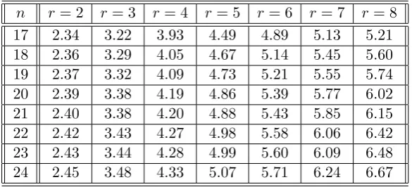
We ran a few experiments to verify the above argument. The value of n is chosen to vary from 17 to 24 and the value of r is chosen to vary from 2 to 8. Table 1 shows the expected header lengths obtained by the CSD algorithm. For each value of n, we considered two possible ways of handling dummy users – all of them privileged and all of them revoked. The results for dummy revoked users is shown in Table 2 and the results for dummy privileged users is shown in Table 3.
In all cases, we observe that the CSD method is never inferior to the SD method with dummy users. In certain cases, the drop in the expected header length of the CSD method as compared to SD method with dummy users can be more than 0.5. While this may not seem very impressive, for actual practical situations, the number of users will be much more and the corresponding improvements will become noticeable. Later we use our algorithm for computing expected header lengths to report results for the CSD scheme for large values of
n. But, there is no corresponding algorithm for the SD scheme with dummy revoked or dummy privileged users with all the dummy users forming a block. One needs to run the SD cover generation algorithm on all possible revocation patterns. It is not possible to do this for large values of n.
4
Counting Revocation Patterns in the CSD method
A given set of revoked users is called arevocation pattern. We denote a revocation pattern onnusers wherer
are revoked, as an (n, r)-revocation pattern. The number of possible (n, r)-revocation patterns is nr. In order to study the behaviour of the CSD algorithm, we find a method to count the number of (n, r)-revocation patterns that result in a cover size (header length) ofh.
In a subtreeTj ofT0 withλ
j users (leaves),N(λj, r, h) is defined as the number of(λj, r)-revocation patterns
that are covered by exactly h subsets. Similarly, forλj users in Tj,T(λj, r, h) is defined as the number of (λj, r)
-revocation patterns that are covered by h subsets such that there is at least one revoked user in both subtrees of
Tj. Since the tree T0 hasn (= λ
0) leaves, N(n, r, h) =N(λ0, r, h) is the number of (n, r)-revocation patterns covered by a header length of h. N(n, r, h) is what we intend to find.
4.1 Few notations
Level number and position of nodes: Before we start computing the values ofT(n, r, h) andN(n, r, h), we fix a few notation for the ease of description. A level number of T0 is indicated by`. At times we will denote the level of a nodeiby`i. The root node 0 is at the highest level`0. Hence, `∈ {0, . . . , `0}. Since every subtree Ti is a complete binary tree, 2`i−1 < λ
i ≤2`i. For the whole tree T0, we see that 2`0−1 < n≤ 2`0. In other words, 2`1 < n≤2`1+1 where `
1 is the level of node 1 (left child of root node). The number of nodes at level ` of T0 is denoted by q`. We see that the number of nodes at the last level is q
0 = 2(n−2`1). For`∈ {1, . . . , `0},
q` = 2`0−`. The position of a node at a level from the left is denoted bykwherek ranges from 1 toq`. Hence, a nodeiis uniquely represented by the pair (`i, ki) – the level `i ofT0 to which it belongs and its positionki from the left at that level. As an example, the root node 0 of T0 is represented by (`
n r = 2 r= 3 r= 4 r = 5 r = 6 r= 7 r= 8 17 2.34 3.22 3.93 4.49 4.89 5.13 5.21 18 2.36 3.29 4.05 4.67 5.14 5.45 5.60 19 2.37 3.32 4.09 4.73 5.21 5.55 5.74 20 2.39 3.38 4.19 4.86 5.39 5.77 6.02 21 2.40 3.38 4.20 4.88 5.43 5.85 6.15 22 2.42 3.43 4.27 4.98 5.58 6.06 6.42 23 2.43 3.44 4.28 4.99 5.60 6.09 6.48 24 2.45 3.48 4.33 5.07 5.71 6.24 6.67
Table 1: The expected header lengths for 17≤n≤24 and 2≤r ≤8 in the CSD method.
n r = 2 r= 3 r= 4 r = 5 r = 6 r= 7 r= 8
17 3.06 3.87 4.49 4.96 5.29 5.46 5.49 18 3.04 3.88 4.53 5.04 5.41 5.65 5.74 19 3.12 4.01 4.72 5.27 5.69 5.97 6.11 20 2.86 3.70 4.40 4.98 5.44 5.80 6.03 21 3.69 4.44 5.07 5.60 6.02 6.35 6.56 22 3.19 4.09 4.86 5.50 6.01 6.40 6.69 23 3.27 4.20 5.01 5.68 6.23 6.66 6.98 24 2.70 3.54 4.35 5.08 5.71 6.24 6.67
Table 2: The expected header lengths for 17≤n≤24 (in each case 32−nrevoked dummy users are added) and 2≤r ≤8 in the SD method.
n r = 2 r= 3 r= 4 r = 5 r = 6 r= 7 r= 8
17 2.76 3.88 4.66 5.24 5.64 5.87 5.96 18 2.67 3.76 4.53 5.09 5.51 5.78 5.92 19 2.61 3.72 4.52 5.16 5.67 6.07 6.35 20 2.56 3.66 4.48 5.15 5.69 6.12 6.44 21 2.52 3.64 4.52 5.26 5.90 6.43 6.84 22 2.49 3.62 4.53 5.31 5.99 6.56 7.03 23 2.47 3.62 4.58 5.41 6.14 6.77 7.28 24 2.45 3.60 4.59 5.45 6.19 6.83 7.34
1 2
6
10
7 14
5 4
3
15 16 17 18 19 20 21 22 23 24
11 12 13
9 8
0
l=1
l=0 l=4
l=3
l=2
Figure 3: Level numbers and the path P0 (with blue) in T0. Nodes coloured blue are at position kP
` for the respective level`.
Non-full subtrees at each level of T0: Let us take a closer look at the structure of the treeT0. In caseT0 is full, all its subtrees are also full. In caseT0 is non-full, we observe that every level` (>0) of T0 can have at most one non-full subtree. To identify these subtrees, we look at the path joining the root node 0 of T0 with node n−2 (the last non-leaf node) and denote it byP0. There is exactly one node onP0 for every level`(>0) of T0. For level `, the position of the node lying on the path P
0 from the left, is denoted by kP` . Let j be a node on P0, say the node represented by (`, kP` ). The part of the pathP0 lying in the subtree Tj is denoted as Pj. For the level`, the subtree Tj rooted at node (`, kP
` ) is the only possibly non-full subtree rooted at level `. The subtrees to the left and right of nodekP` at level`are all full. The subtrees to the left (right) of nodekP` of level ` have 2` (respectively 2`−1) leaves. The number of leaves in the only possibly non-full subtree rooted at level` (subtree rooted at node (`, kP` ) of level `) is denoted byλ`,P. Hence, 2`−1 < λ`,P ≤2`. More specifically,
λ`,P =n−((k`P−1)×2`)−((2`0−`−kP
` )×2`
−1). Also,kP
` =
q0
2`
. We definekPj
` for the pathPj as the position of the node at level` onPj from the left in the subtreeTj. Hence,k`P is also denoted ask
P0
` . One can see that
kPj ` =
&
q0−(kP`j−1)×(2`j)
2`
'
=q0
2`
−(kP`
j−1)×(2 `j−`).
4.2 Recurrences N(n, r, h) and T(n, r, h)
Theorem 1. For a subtree Ti of T0 withλ
i (2` < λi≤2`+1) leaves,
N(λi, r1, h1) =T(λi, r1, h1) +
X
j∈IN(i)
T(λj, r1, h1−1) (1)
where IN(i) is the set of all internal nodes in the subtreeTi excluding the node i.
Now, let us consider a (λi, r)-revocation pattern that has been counted in T(λi, r, h). By the definitions of
T and N, the (λi, r)-revocation patterns that are counted in T(λi, r, h) are also counted inN(λi, r, h). For some other revocation pattern, counted in T(λj, r, h−1) (for some j ∈ IN(i)), both subtrees of Tj contain at least one revoked user in each. Hence, the minimal subtree ofTi containing the r revoked users for such a revocation pattern isTj. For the revocation patterns counted in T(λ
j, r, h−1), the privileged users of the subtreeTj have been covered withh−1 SD subsets of S. The rest of the λi−λj users are all privileged and are covered by one more SD subsetSi,j. Hence, the corresponding (λi, r)-revocation pattern is counted in N(λi, r, h).
Theorem 2. For a subtree Ti of T0 withλ
i (2` < λi≤2`+1) leaves,
T(λi, r1, h1) = r1−1
X
r0=1 h1
X
h0=0
N(λ2i+1, r0, h0)×N(λ2i+2, r1−r0, h1−h0) (2)
where λ2i+1 (respectively λ2i+2) is the number of leaves in the left (respectively right) subtree of Ti.
Proof. We show that a revocation pattern is counted in T(λi, r1, h1) if and only if it is counted in the right hand side of (2). For a given λi, the number of leaves in the left and right subtrees get fixed to λ2i+1 and
λ2i+2 respectively. When a (λi, r1)-revocation pattern is counted in T(λi, r1, h1), both the subtrees of Ti must have at least one revoked user. Assuming the left subtree of Ti has r0 revoked users, the right subtree should
have r1−r0 revoked users since the total number of revoked users isr1. Similarly, assuming that the privileged users in this left subtree are covered by h0 sets of S, the privileged users in the right subtree should be covered by h1 −h0 sets of S. The number of (λ2i+1, r0)-revocation patterns in the left subtree covered by h0 subsets is N(λ2i+1, r0, h0). Similarly, the number of (λ2i+2, r1 −r0)-revocation patterns in the right subtree covered by
h1−h0 subsets isN(λ2i+2, r1−r0, h1−h0). Each such (λ2i+1, r0)-revocation pattern in the left subtree along with a (λ2i+2, r1−r0)-revocation pattern in the right subtree gives rise to a (λi, r)-revocation pattern in the treeTi that is covered byh1 subsets ofS. Hence, for all values of r0 ∈ {1, . . . , r1−1} and all values of h0 ∈ {0, . . . , h1},
N(λ2i+1, r0, h0)×N(λ2i+2, r1−r0, h1−h0) counts all the possible T(λi, r1, h1).
Any (λi, r1)-revocation pattern covered by h0 subsets will be counted in someN(λ2i+1, r0, h0)×N(λ2i+2, r1−
r0, h1−h0). The ones counted inN(λ2i+1, r0, h0)×N(λ2i+2, r1−r0, h1−h0) for fixed values ofr0andh0 are counted exactly once in it. For other values of r0 and h0, the corresponding (λi, r1)-revocation patterns will be counted in the respective N(λ2i+1, r0, h0)×N(λ2i+2, r1−r0, h1−h0). Hence, a (λi, r1)-revocation pattern is counted on the right hand side of (2) if and only if it is counted in T(λi, r1, h1).
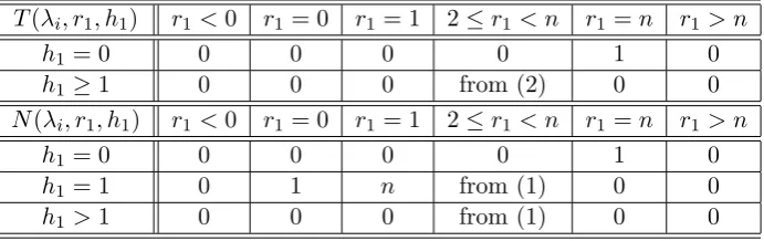
Boundary conditions: The boundary conditions onT(λi, r1, h1) andN(λi, r1, h1) are given in Table 4. Other than the tabulated values, N(λi, r1, h1) = 0 for λi ≤ 0 and T(λi, r1, h1) = 0 for λi ≤ 1. From recurrences in Theorems (1) and (2) and the boundary conditions on these recurrences, one can find the value ofN(n, r, h) for any given n,r and h using dynamic programming.
4.3 Algorithms to compute N(n, r, h) and T(n, r, h)
Substituting for j ∈ IN(i): To use these recurrences as an algorithm, the nodes j ∈ IN(i) in (1) for a node
i have to be explicitly identified and the corresponding λjs have to be substituted. As described in section 4.1 before, there are at most three types of subtrees rooted at a level`j ofT0: full subtrees of height`i, full subtrees of height`i−1 and a non-full complete subtree of height`i.
(1) For a subtree Ti that is full and is of height 2`i (to the left of the node at position kP
`i at level`i):
N(λi, r1, h1) =T(λi, r1, h1) + `i−1
X
`j=1
(2`i−`j)×T(2`j, r
T(λi, r1, h1) r1<0 r1 = 0 r1= 1 2≤r1 < n r1 =n r1 > n
h1= 0 0 0 0 0 1 0
h1≥1 0 0 0 from (2) 0 0
N(λi, r1, h1) r1<0 r1 = 0 r1= 1 2≤r1 < n r1 =n r1 > n
h1= 0 0 0 0 0 1 0
h1= 1 0 1 n from (1) 0 0
h1>1 0 0 0 from (1) 0 0
Table 4: Boundary conditions on T(n, r, h) andN(n, r, h).
(2) For a subtree Ti that is full and is of height 2`i−1 (to the right of the node at position kP
`i at level`i):
N(λi, r1, h1) =T(λi, r1, h1) + `i−1
X
`j=2
(2`i−`j)×T(2`j−1, r
1, h1−1). (4)
(3) For the only possibly non-full subtree Ti fori= (`
i, kP`i) of height 2`i (at position kP`i at level`i):
N(λi, r1, h1) =T(λi, r1, h1)
+ `i−1
X
`j=2 [(kPi
`j −1)×T(2 `j, r
1, h1−1) +T(λ`j,P, r1, h1−1) + (2`i−`j−kPi
`j)×T(2 `j−1, r
1, h1−1)]. (5)
Dynamic Programming: ComputingN(n, r, h) andT(n, r, h) requires computingN(λi, r1, h1) andT(λi, r1, h1) for some smaller λi, r1 and h1. We use dynamic programming technique where all values of N(λi, r1, h1) and
T(λi, r1, h1) for smaller λi, r1 and h1 are pre-computed. The algorithm to compute T(n, r, h) from these pre-computed values is obtained from (2) in a straight forward manner. The algorithm to compute N(n, r, h) from these pre-computed values is obtained from (1) (more specifically from either of (3) or (5)). Level `i of T0 has
kP`
i−1 full subtrees of height`i, (2
`0−`i)−kP
`i full subtrees of height`i−1 and one possibly non-full subtree. For every level in the tree T0,T(λ
i, r, h−1) is pre-computed once for each of the three types of nodes and used to compute N(n, r, h).
Space and Time complexity of the algorithm: Using (2) to compute T(n, r, h) from the pre-computed values of N(·,·,·) requires O(rh) memory operations and multiplications. Equation (1) shows how N(n, r, h) is related to pre-computed values of T(·,·,·). Actual computation is done using (3), (4) and (5). This requires
O(1) memory operations and a single addition for each of the dlogne levels of T0. Hence, the time complexity for computing T(n, r, h) and then N(n, r, h) from pre-computed values isO(rh+ logn).
These pre-computed values in turn need to be computed. By the form of (3), (4) and (5) there are logn
subtrees to be considered. For each such subtree,O(rh) values need to be computed and the computation of these will be based on values computed earlier. A dynamic programming algorithm proceeds in a bottom-up fashion by computing the O(rh) values corresponding to smaller sub-trees and then using these to compute the values for progressively larger sub-trees. This takes a total of O(r2h2logn+rhlog2n) time. The space requirement is given by the number of pre-computed values that need to be stored to compute N(n, r, h). For each of the
n r h N(n, r, h) 126 63 37 7.44×1035 127 61 37 1.27×1036 128 64 37 2.96×1036 131 65 38 2.33×1037
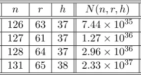
Table 5: Listing a few values ofn,r,h and their correspondingN(n, r, h).
The above time and space complexities are required for a single set of values ofn,rand h. For a fixednand
r, it may be required to compute the values of N(n, r, h) for all possible values of h. This would be a typical requirement for a broadcast centre which will have a fixed number of users and for a particular transmission knows the number of revoked users. The corresponding time and space complexities can be obtained by substituting an appropriate value forh. A trivial bound is n; but, later we show thath≤2r−1 which gives the expressions
O(r4logn+r2logn) and O(r2log2n) for time and space complexities respectively. For large n and moderate values of r, these are practical complexities.
Further, allowing r to range over all the O(n) possible values leads to O(n4logn+n2log2n) time and
O(n2logn) space complexities respectively. If we are interested in computingN(i, r, h) for all 2≤i≤nand all possible values of r and h, then the time and space complexities areO(n5+n3logn) and O(n3) respectively.
Table 5 lists the values of n, r, h and their corresponding N(n, r, h) for some values of n, r and h. Note that computing these values would not be possible by direct enumeration. For example, attempting direct enumeration to tackle the first row of Table 5, would require considering 12663 possible revocation patterns which is way beyond the present computational capabilities.
4.4 Upper Bounds on Header Length of the (C)SD method
We first prove that the header length of the CSD scheme is upper bounded by 2r−1. For full trees of the SD method, this bound was proved in [NNL01].
Theorem 3. N(λi, r1, h1) = 0 when h1 >2r1−1. T(λi, r1, h1) = 0 when h1 ≥2r1−1.
Proof. First we show that T(λi, r1, h1) = 0 when h1 ≥ 2r1 −1 in (1). We prove this from (2) by induction on r1. The boundary conditions have been listed in Table 4. We know that, 2`i−1 < λi ≤ 2`i. By induction hypothesis, when h0 >2r0−1 and 1≤r0 < r1,N(λ2i+1, r0, h0) = 0. If h0 ≤2r0−1, thenh1−h0 >2r1−1−h0 ≥ 2r1−1−2r0+ 1 = 2(r1−r0). Then, again by induction hypothesis,N(λ2i+2, r1−r0, h1−h0) = 0. Hence, when
h1≥2r1−1,T(λi, r1, h1) = 0.
Now, ifh1>2r1−1, the other terms on the right hand side of (1) areT(λi, r1, h1−1) where h1−1≥2r1−1 for all terms and hence are all 0 as proved above. Hence, whenh1>2r1−1, N(λi, r1, h1) = 0.
We later show that for sufficiently large n, N(n, r,2r−1) is positive and also characterize the minimum n
for which this happens.
Next, we show thatN(n, r, h) is monotonic onnfor fixedr and h. While intuitive, there does not seem to be an easy way to prove this.
Proof. Let T(n2, r, h)6= 0. From (2) we get:
T(n2, r, h) = r−1
X
r0=1 h
X
h0=0
N(λ1, r0, h0)×N(λ2, r−r0, h−h0).
LetRH ={(r1, h1). . . ,(rs, hs)} be such that bothN(λ1, r0, h0) andN(λ2, r−r0, h−h0) are non-zero (and hence
N(λ1, r0, h0)×N(λ2, r−r0, h−h0) is non-zero) when (r0, h0)∈RH. Hence, we can also write:
T(n2, r, h) =
X
(r0,h0)∈RH
N(λ1, r0, h0)×N(λ2, r−r0, h−h0).
Sinceλ1< n2(by the structure ofT0withn2leaves), hence by induction hypothesis, for anyλ≥λ1,N(λ1, r, h)6= 0 implies N(λ, r, h)6= 0. Similarly, since λ2 < n2, hence by induction hypothesis, for anyλ≥λ2,N(λ2, r, h)6= 0 implies N(λ, r, h) 6= 0. When there are n1 leaves in the tree let there be λ01 leaves in the left subtree and λ02 leaves in the right subtree of the root node. Hence, by the construction of T0, we get λ0
1 ≥λ1 and λ02 ≥λ2. In the expression for T(n1, r, h), for (r0, h0) ∈RH, by induction hypothesis, N(λ10, r0, h0) and N(λ20, r−r0, h−h0) are both non-zero. Hence, for at least (r0, h0) ∈ RH, N(λ01, r0, h0) ×N(λ02, r−r0, h−h0) is non-zero. Thus,
T(n1, r, h)6= 0.
Now, letN(n2, r, h)6= 0. From (1) we get:
N(n2, r, h) =T(n2, r, h) + n2−2
X
j=1
T(λj, r, h−1).
Let I = {i1, . . . , it} be the nodes of T0 (with n2 leaves) such that T(λi, r, h) 6= 0 for i ∈ I. By induction hypothesis, for anyλj < n2 andλi > λj, ifT(λj, r, h)6= 0 thenT(λi, r, h)6= 0. Hence, we can also write:
N(n2, r, h) =T(n2, r, h) +
X
i∈I
T(λi, r, h−1).
Here, T(n2, r, h) 6= 0 implies T(n1, r, h) 6= 0 by the first part of this proof. By the construction of the tree T0,
λ0i ≥λi where λi0 is the number of leaves (users) in the subtree rooted at nodei of the tree T0 for n1 users. By induction hypothesis, at least for i∈I, sinceT(λi, r, h−1)6= 0, henceT(λ0i, r, h−1)6= 0. Thus,N(n1, r, h)6= 0.
Now, we prove that ifr is not small compared to n, thenT(n, r,2r−2) = 0.
Lemma 5. For n≤22k+1 and r >2k, T(n, r,2r−2) = 0.
Proof. For T(n, r,2r−2) in (2), let h0 <2r0−1, thenh−h0 = 2r−2−h0 >2r−2−2r0+ 1 = 2(r−r0)−1. Hence by Theorem 3, N(λ2, r−r0, h−h0) = 0. Similarly, if h0 >2r0−1,N(λ1, r0, h0) = 0. So, in the expression forT(n, r,2r−2), the terms on the right hand side of (2) are 0 ifh06= 2r0−1. Hence,
T(n, r,2r−2) = r−1
X
r0=1
N(λ1, r0,2r0−1)×N(λ2, r−r0,2(r−r0)−1). (6)
Now by induction onλi, we prove thatN(λ1, r0,2r0−1) = 0 andN(λ2, r−r0,2(r−r0)−1) = 0. The boundary conditions have been listed in Table 4. By induction hypothesis, forλi≤22m+1 wherem < k andr0 >2m let us assumeT(λi, r0,2r0−2) = 0. In (6), letr0 ≥ r2 which impliesr0>2k−1. Hence, forλi ≤22k−1,T(λi, r0,2r0−2) = 0 by the induction hypothesis. Also, by Theorem 3, T(λ1, r0,2r0−1) = 0. Putting these values in (1), we get
Some insight: Given a revocation pattern, if we revoke one more user from it, that can result in either increase, decrease or no change in the cover size. Increase in cover size mostly happens when the newly revoked user is not adjacent to any previously revoked user. The cover size remains unchanged or decreases when the newly revoked user is adjacent to a previously revoked user. Decrease in cover size happens when the user in a singleton subset of the cover is revoked. As the number of revoked users increase, the maximum possible cover size for that number of revoked users increases up to a certain point. After that the maximum possible cover size decreases. One may also observe that forn >2 (`1≥1),q0/2 =n−2`1. Since 2`1 is even for`1 ≥1, hence whennis even
q0/2 is even and when nis odd q0/2 is odd.
Theorem 6. The header length in the CSD method for n users is at most n
2
irrespective of the number of revoked users.
Proof. First, we show that N(n, r, h) = 0 for h > n2 for any r. We prove this by induction on n. From (1) we have:
N(n, r, h) =T(n, r, h) + n−2
X
i=1
T(λi, r, h−1)
and hence,T(n, r, h)≤N(n, r, h). Whenλi < nandh−1≥
n
2
,N(λi, r, h−1) = 0. Thus,Pin=1−2T(λi, r, h−1) = 0. From (2) we get:
T(n, r, h) = r−1
X
r0=1 h
X
h0=0
N(λ1, r0, h0)×N(λ2, r−r0, h−h0).
When h0 > λ1
2 , N(λ1, r
0, h0) = 0 by induction hypothesis. When h0 ≤ λ1
2 , sinceh > n
2, h−h
0 > n 2 −
λ1
2 = λ2
2 . Therefore, N(λ2, r−r0, h−h0) = 0 by induction hypothesis. Hence, N(n, r, h) = 0 for h > n2 for any r.
Next, we show that the upper bound ofn2is actually achieved. First let us assume thatnis even and hence
q0/2 is even. We construct a revocation pattern such that none of the users are revoked initially. Now, let us form a revocation pattern by revoking one user from each of the q0/2 subtrees rooted at level q1 with leaves at level q0 and one user each from subtrees rooted at level 2 with leaves at level 1. Since all the privileged users would form singleton subsets in the cover for this revocation pattern, hence the header length for the revocation pattern thus constructed is of size q1 (= n2). Now, if we attempt to revoke any other user, then by pigeonhole principle, one of the sets in the cover gets removed and hence the header length decreases. Hence, for even n, the maximum header length is n2.
For oddn, q0/2 is odd. We construct a revocation pattern similarly by revoking one user from each of the
q0/2 subtrees rooted at level q1 with leaves at level q0 and one user each from subtrees rooted at level 2 with leaves at level 1. Since q0/2 is odd, there will be one subtree (rooted at the node at position k2P) with leaves at both levels 0 and 1. For this subtree, only one out of the three users in it is revoked. Since all the privileged users would form singleton subsets (except the one generated from the above subtree) in the cover for this revocation pattern, hence the cover size for the revocation pattern thus constructed is of size q1 (=
n
2
). This is again the maximum header length by the same argument as above.
Hence, the maximum header length isn2fornusers.
Theorem 6 gives a bound on the header size. Previously, the bound of 2r−1 for the header size had been obtained. The next result completes the picture by obtaining yet another bound on the header size.
Theorem 7. The maximum header length in the CSD method for n users is min(2r−1,n
2
, n−r).
Proof. The bounds 2r−1 anddn/2ehave already been shown. We show the bound ofn−r on the header size. The proof of this is similar to the first part of the proof of Theorem 6, i.e., we show that N(n, r, h) = 0 for
Forλi < n, we have h−1> n−1−r≥λi−r and hence using induction, N(λi, r, h−1) = 0 which implies thatT(λi, r, h−1) is also zero. Again, consider the value ofT(n, r, h) and the recurrence expressing this in terms ofN(λ1, r0, h0) andN(λ2, r−r0, h−h0), whereλ1+λ2 =n. Ifh0 > λ1−r0, then using induction,N(λ1, r0, h0) = 0. So, suppose that h0 ≤λ1−r0. Usingh > n−r, we have h−h0 >(n−λ1)−(r−r0) =λ2−(r−r0) and again using induction,N(λ2, r−r0, h−h0) = 0.
This shows that T(n, r, h) = 0 which combined with the fact that the other relevant values of T(·,·,·) are zero, shows that N(n, r, h) = 0 for h > n−r.
The bound given by Theorem (7) gives a complete picture. Ifr ≤n/4, then the bound 2r−1 is appropriate; ifn/4< r≤n/2, then the bound dn/2e is appropriate; and for r > n/2, the bound (n−r) is appropriate. The last bound has an important consequence. If the number of revoked users is greater than n/2, it may appear that using individual transmission to the privileged users would be better than using the CSD method. But, The bound of (n−r) on the header size shows that this is not true. Using the CSD method is never worse than individual transmission to privileged users.
The bound of Theorem 7 hold for the SD scheme, i.e., for full trees. We note that the only previouslyproved
upper bound for the SD scheme is 2r−1. The other two bounds bounds, while intuitive, do not appear to have been reported with proofs in the literature. In fact, there does not seem to be an easy way to argue about these bounds without using the recurrences that we have derived.
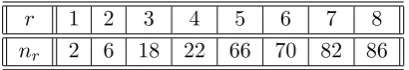
Definition 1. nr: For a given r, nr is the minimum number of users required to be in the system so that there
exists an (n, r)-revocation pattern covered by a header length of2r−1. In other words, nr is the minimum nfor
which N(n, r,2r−1)>0.
Theorem 3 shows that the upper bound on the header length is 2r−1. By characterizing nr, we show that this upper bound on h is actually achieved.
Lemma 8. In the CSD method, 2k−1 < r≤2k if and only if 22k< nr <22k+1.
Proof. We first prove that if 2k−1 < r ≤2k, then 22k < nr ≤22k+1 (by showing that N(22k, r,2r−1) = 0 and
N(22k+1, r,2r−1)6= 0). Although by Theorem 3,T(22k+1, r,2r−1) = 0, we show that T(22k, r,2r−2)6= 0 and hence at least one of the terms on the right hand side of (1) is non-zero and hence N(22k+1, r,2r−1)6= 0. From (2) we get:
T(22k, r,2r−2) = r−1
X
r0=1 2r−2
X
h0=0
N(22k−1, r0, h0)×N(22k−1, r−r0,2r−2−h0).
Whenh0 >2r0−1,N(22k−1, r0, h0) = 0 by Theorem 3. Similarly, whenh0<2r0−1, 2r−2−h0 >2r−2−2r0+ 1 = 2(r−r0)−1 and hence N(22k−1, r−r0,2r−2−h0) = 0. Hence, we get
T(22k, r,2r−2) = r−1
X
r0=1
N(22k−1, r0,2r0−1)×N(22k−1, r−r0,2(r−r0)−1).
When r0 = dr 2e (2
k−2 < r0 ≤ 2k−1) by induction hypothesis, n
r0 ≤ 22k−1 and hence by Lemma 4, both
N(22k−1, r0,2r0 −1) and N(22k−1, r−r0,2(r −r0)−1) are non-zero. Hence, T(22k, r,2r−2) 6= 0 which im-plies N(22k+1, r,2r−1) 6= 0. Since T(nr, r,2r−1) = 0 and T(22k−1, r,2r−2) = 0 hence, nr < 22k+1. Next, we show that N(22k, r,2r−1) = 0. By Theorem 3, T(22k, r,2r−1) = 0. By Lemma 5, for all λi ≤ 22k−1 and
r >2k−1,T(λi, r,2r−2) = 0 and henceN(22k, r,2r−1) = 0.
Next, we prove that for some 22k < nr ≤ 22k+1, the corresponding r is such that 2k−1 < r ≤ 2k. Let the corresponding r be such that 2k0−1 < r ≤ 2k0 where k 6= k0. Then by the argument above, we know that 22k0 < nr≤22k
0+1
which is a contradiction sincenris unique for a givenrby definition. Hence the corresponding
r 1 2 3 4 5 6 7 8
nr 2 6 18 22 66 70 82 86
Table 6: Listing a few values of r and their correspondingnr.
One may note here that not all n between 2k−1 and 2k is an n
r for some r. We list a few r and their correspondingnr in Table 6. Next, we find an expression for nr.
Theorem 9. In the CSD method, let 2k−1 < r ≤2k. When r ≤2k−1+ 2k−2, letr1 = 2k−2 and r0 =r−2k−2
and hence,
nr=nr0+ 2
2k−2+ 22k−1
and when r >2k−1+ 2k−2, letr0= 2k−1 andr1 =r−2k−1 and hence,
nr = 22k−1+nr1 + 2
2k−1.
Proof. From Lemma 8 we know that for 2k−1 < r≤2k, 22k< nr ≤22k+1. For such annr, λ1 =nr−22k−1 and
λ2= 22k−1. From (1) we get
N(nr, r,2r−1) =T(nr, r,2r−1) +T(nr−22k−1, r,2r−2) +T(22k−1, r,2r−2) + nr−2
X
i=3
T(λi, r,2r−2).
From Theorem 3 we know thatT(nr, r,2r−1) = 0. From Lemma 5 we know that whenr >2k−1 andλi ≤22k−1,
T(λi, r,2r−2) = 0. Hence the only non-zero component is T(nr−22k−1, r,2r−2). From (2) we get
N(nr, r,2r−1) =T(nr−22k−1, r,2r−2) = r−1
X
r0=1 2r−2
X
h0=0
N(λ3, r0, h0)×N(λ4, r−r0,2r−2−h0).
By an argument similar to the one used in the proof for Lemma 8, we get
N(nr, r,2r−1) =T(nr−22k−1, r,2r−2) = r−1
X
r0=1
N(λ3, r0,2r0−1)×N(λ4, r−r0,2(r−r0)−1).
By the construction of the complete treeT0 and the fact thatT2 does not have any revoked user (T(22k−1, r,2r− 2) = 0) it can be seen that 22k−2 < λ3 ≤22k−1 and 22k−2 ≤λ4 <22k−1.
When r ≤ 2k−1 + 2k−2, let r0 = r0 = r −2k−2 and r −r0 = r1 = 2k−2. From the construction of the complete tree T0 for (n
r0 + 2
2k−2 + 22k−1) users, it can be seen that λ
3 = nr0 and λ4 = 2
2k−2. Hence,
N(λ3, r0,2r0−1) =N(nr0, r0,2r0−1)6= 0 by the definition of nr. Also, from Lemma 4 and Lemma 8 we know
that for r = 2k (consequently nr <22k+1) and λ≥ 22k+1, N(λ, r,2r−1)6= 0. So for r1 = r−r0 = 2k−2 and
λ4 = 22(k−2)+2 we get, N(λ4, r−r0,2(r−r0)−1) = N(22k−2, r1,2r1 −1) 6= 0. Hence, for r ≤ 2k−1+ 2k−2,
N(nr, r,2r−1)6= 0 wherenr=nr0 + 2
2k−2+ 22k−1.
Now, we show that for 2k−1 < r ≤ 2k−1+ 2k−2 (r0 = r−2k−2 and r1 = 2k−2), N(nr−1, r,2r−1) = 0. In the tree T0 for (n
r0 + 2
2k−2 + 22k−1)−1 users, λ
3 = nr0 −1 and λ4 = 2
2k−2. Since there are n r0 −1
users in T3, at most r
0−1 revoked users can be accommodated in T3 so that N(λ3, r0,2r0−1)6= 0 and hence
r0 =r0−1 andr−r0 = 2k−2+ 1. By Lemma 8 for r−r0 >2k−2, nr−r0 > 22k−2. But, λ4 = 22k−2 and hence
When r > 2k−1 + 2k−2, let r0 = r0 = 2k−1 and r−r0 = r1 = r −2k−1. From the construction of the complete tree T0 for (22k−1 +n
r1 + 2
2k−1) users, it can be seen that λ
3 = 22k−1 and λ4 = nr1. Hence,
N(λ4, r−r0,2(r−r0)−1) =N(nr1, r1,2r1−1) 6= 0 by the definition of nr. From Lemma 4 and Lemma 8 we
know that for r = 2k (consequently nr <22k+1) and λ≥22k+1, N(λ, r,2r−1)6= 0. So for r0 =r0 = 2k−1 and
λ3= 22(k−1)+1we get,N(λ3, r0,2r0−1) =N(22k−1, r0,2r0−1)6= 0. Hence, forr >2k−1+2k−2,N(nr, r,2r−1)6= 0 wherenr = 22k−1+nr1 + 2
2k−1.
Now, we show that for r >2k−1+ 2k−2 (r0 = 2k−1 and r1 =r−2k−1), N(nr−1, r,2r−1) = 0. In the tree T0 for (22k−1+n
r1+ 2
2k−1)−1 users,λ
3= 22k−1 and λ4 =nr1−1. Since there arenr1−1 users inT
4, at most
r1−1 revoked users can be accommodated inT4 so thatN(λ4, r−r0,2(r−r0)−1)6= 0 and hencer−r0 =r1−1 and r0 = 2k−1+ 1. By Lemma 8 for r0 >2k−1, nr0 >22k−1. But, λ3 = 22k−1 and hence N(λ3, r0,2r0−1) = 0. Consequently, we getN(nr−1, r,2r−1) = 0.
Note that for the SD method, when 2k−1 < r ≤ 2k, the minimum n for which the header length of 2r−1 occurs is 22k+1. This has been earlier proved in [PB06]. It is because the CSD method allows arbitrary number of users, the value ofnfor which the maximum header length of 2r−1 is achieved for a given r is less than that of the SD method.
4.5 Generating Function from Recurrences of the CSD scheme for Full Binary trees
Let the number of users ben= 2`0 and hence the treeT0is full and of height`
0. For a full treeT0, all subtrees Ti are full and at level `, there are 2`0−` subtrees with 2` leaves in each. We define T
`(r, h) = T(2`, r, h) and
N`(r, h) =N(2`, r, h). Then the recurrences (1) and (2) for counting the number of revocation patterns become:
N`0(r, h) =T`0(r, h) +
`0−1
X
`=1
2`0−`×T
`(r, h−1)
. (7)
T`0(r, h) =
r−1
X
r1=1
h
X
h1=0
N`0−1(r1, h1)×N`0−1(r−r1, h−h1) (8)
wherer is the number of revoked users.
Theorem 10. The generating function for the sequence N`0(r, h) of numbers defined in (7) above, is given by
X`0(x, y) where
X`0(x, y) =
X`0−1(x, y)−xy
2`0−12
+xy2`0 + 2`0x2y2`0−1+
`0−1
X
`=1
2`0−`xy2`0−2`×X
`−1(x, y)−xy2
`−12 .
Proof. Let Y`0(x, y) be the generating function for the sequenceT`0(2
`0 −r, h) defined as follows:
Y`0(x, y) =
2`0
X
r=0 2`0−r
X
h=0
T`0(r, h)x
hy2`0−r
and the generating functionX`0(x, y) for the sequence N`0(2
`0−r, h) can be written as:
X`0(x, y) =
2`0
X
r=0 2`0−r
X
h=0
N`0(r, h)x
hy2`0−r
. (10)
By definition, when `0 = 0, Y0(x, y) = 0 and X0(x, y) = 1 +xy and when `0 = 1, Y1(x, y) = 1 andX1(x, y) = 1 + 2xy+xy2.
Now, we note that:
X`20−1(x, y) = 2`0−1
X
r1=0
2`0−1−r 1
X
h1=0
N`0−1(r1, h1)x
h1y2`0−1−r1×
2`0−1
X
r2=0
2`0−1−r 2
X
h2=0
N`0−1(r2, h2)x
h2y2`0−1−r2
=N`0−1(0,1)xy
2`0−1
+ 2`0−1
X
r1=1
2`0−1−r 1
X
h1=0
N`0−1(r1, h1)x
h1y2`0−1−r1
×
N`0−1(0,1)xy
2`0−1
+ 2`0−1
X
r2=1
2`0−1−r 2
X
h2=0
N`0−1(r2, h2)x
h2y2`0−1−r2
(11)
PuttingN`0−1(0,1) = 1 in (11) we get:
X`20−1(x, y) = 2`0−1
X
r1=1
2`0−1−r 1
X
h1=0
N`0−1(r1, h1)x
h1y2`0−1−r1×
2`0−1
X
r2=1
2`0−1−r 2
X
h2=0
N`0−1(r2, h2)x
h2y2`0−1−r2
+xy2`0−1
2`0−1
X
r2=1
2`0−1−r2
X
h2=0
N`0−1(r2, h2)x
h2y2`0−1−r2
+xy2`0−1
2`0−1
X
r1=1
2`0−1−r1
X
h1=0
N`0−1(r1, h1)x
h1y2`0−1−r1
+x2y2`0 (12)
Let
C`0(x, y) =
2
`0−1
X
r1=1
2`0−1−r1
X
h1=0
N`0−1(r1, h1)x
h1y2`0−1−r1×
2`0−1
X
r2=1
2`0−1−r2
X
h2=0
N`0−1(r2, h2)x
h2y2`0−1−r2
= 2`0
X
r=2 2`0−r
X
h=0
xhy2`0−r
r−1
X
r1=1
h
X
h1=0
Now we take a closer look at the generating functionY`0(x, y) of (9):
Y`0(x, y) =
2`0
X
r=0 2`0−r
X
h=0
T`0(r, h)x
hy2`0−r
= 2`0
X
r=0 2`0−r
X
h=0
xhy2`0−r
r−1
X
r1=1
h
X
h1=0
N`0−1(r1, h1)×N`0−1(r−r1, h−h1)
= 2`0
X
r=0 2`0−r
X
h=0
xhy2`0−r
r−1
X
r1=1
h
X
h1=0
N`0−1(r1, h1)×N`0−1(r−r1, h−h1)
= 2`0
X
r=2 2`0−r
X
h=0
xhy2`0−r
r−1
X
r1=1
h
X
h1=0
N`0−1(r1, h1)×N`0−1(r−r1, h−h1)
+ 1
X
r=0 2`0−r
X
h=0
xhy2`0−r
r−1
X
r1=1
h
X
h1=0
N`0−1(r1, h1)×N`0−1(r−r1, h−h1)
= 2`0
X
r=2 2`0−r
X
h=0
xhy2`0−r
r−1
X
r1=1
h
X
h1=0
N`0−1(r1, h1)×N`0−1(r−r1, h−h1) (14)
In (14) above,P1
r=0
P2`0−r h=0 xhy2
`0−rPr−1
r1=1
Ph
h1=0N`0−1(r1, h1)×N`0−1(r−r1, h−h1) = 0. The minimum
value ofr1 orr−r1 is 1. The maximum value forr1 orr−r1 such thatxhy2
`0−r
will have a non-zero coefficient
N`0−1(r1, h1)×N`0−1(r−r1, h−h1) is 2
`0−1.
Hence,C`0(x, y) =Y`0(x, y).
LetA`0−1(x, y) =
P2`0−1
r=1
P2`0−1−r
h=0 N`0−1(r, h)x
hy2`0−1−r. It can be easily seen that
X`0−1(x, y) =
2`0−1
X
r=0
2`0−1−r
X
h=0
N`0−1(r, h)x
hy2`0−1−r
= 2`0−1
X
h=0
N`0−1(0, h)x
hy2`0−1
+ 2`0−1
X
r=1
2`0−1−r
X
h=0
N`0−1(r, h)x
hy2`0−1−r
=xy2`0−1+A`0−1(x, y) (15)
Putting the value ofA`0−1(x, y) from (15) and the value of Y`0 from (14) into (12), we get:
Y`0(x, y) =X
2
`0−1(x, y)−2xy
2`0−1
X`0−1(x, y)−x
2y2`0
=
X`0−1(x, y)−xy
2`0−12
. (16)
Now, to find another relation between the generating functionsX`0(x, y) andY`0(x, y), we multiply both sides
of (7) withxhy2`0−r and sum both sides over 2≤r≤2`0 and 0≤h≤2`0:
2`0
X
r=2 2`0−r
X
h=1
N`0(r, h)x
hy2`0−r= 2`0
X
r=2 2`0−r
X
h=1
T`0(r, h)x
hy2`0−r+ 2`0
X
r=2 2`0−r
X
h=1 `0−1
X
`=1
2`0−`xhy2`0−r×T
`(r, h−1)
Adding the values ofN`0(r, h) andT`0(r, h)(= 0) forr <2 andh≥1 to both sides of the (17) above, we get:
2`0
X
r=0 2`0−r
X
h=1
N`0(r, h)x
hy2`0−r
=xy2`0 + 2`0x2y2`0−1
+ 2`0
X
r=0 2`0−r
X
h=1
T`0(r, h)x
hy2`0−r +
2`0
X
r=0 2`0−r
X
h=1 `0−1
X
`=1
2`0−`xhy2`0−r×T
`(r, h−1)
.
Since forh= 0, N`0(2
`0,0) = 1 (T
`0(2
`0,0) = 1) and for anyr <2`0,N
`0(r,0) = 0 (T`0(r,0) = 0),
X`0(x, y)−1 =xy
2`0
+ 2`0x2y2`0−1+Y
`0(x, y)−1 +
`0−1
X
`=1
2`0 −`×
2`0
X
r=0 2`0−r
X
h=1
T`(r, h−1)xhy2`0−r
=xy2`0 + 2`0x2y2`0−1+Y
`0(x, y)−1 +
`0−1
X
`=1
2`0
−`xy2`0−2`
× 2`
X
r=0
2`0−r−1
X
h=0
T`(r, h)xhy2`−r
. (18)
Since 2`0−r−1>2`−r for 1≤`≤`
0−1, hence we get:
X`0(x, y) =xy
2`0
+ 2`0x2y2`0−1+Y
`0(x, y) +
`0−1
X
`=1
2`0−`xy2`0−2`×Y`(x, y)
. (19)
From (16) and (19) above, we get:
X`0(x, y) =
X`0−1(x, y)−xy
2`0−12
+xy2`0 + 2`0x2y2`0−1+
`0−1
X
`=1
2`0−`xy2`0−2`×X
`−1(x, y)−xy2
`−12 .
(20)
A similar generating function was found by Park and Blake in [PB06]. It was derived based on the structural properties of the tree used in creating the subsets of the subset difference method. We have taken a different approach of first finding the recurrence relations for the sequence N(n, r, h) and then deriving the generating function from it. Our generating function is of a slightly different form.
5
Expected Header Length in the CSD method
Given the number of users n (2`1 < n ≤ 2`1+1), and the number of revoked users r, there are n
r
possible revocation patterns. Each such revocation pattern gives rise to a subset cover for the privileged users and hence a header in the ciphertext C. We now find the expected value of the header length hfor a given nand r.
5.1 Basic Analysis
The Random Experiment: We consider the random experiment where r out of the n initially un-revoked leaves of the treeT0are chosen uniformly at random without replacement and revoked. This gives rise to an (n, r )-revocation pattern and hence a corresponding subset cover Sc and its header lengthh. LetXn,r be the random variable taking the value of the header length h due to the (n, r)-revocation pattern of the above experiment. Next, we associate a random variable with each node of the tree T0. Let Xi


![Table 7: E[Xn,r]rfor given n and r computed using Algorithm 1 for the CSD scheme.](https://thumb-us.123doks.com/thumbv2/123dok_us/1877192.1244478/26.595.211.383.91.184/table-rfor-given-computed-using-algorithm-csd-scheme.webp)