Expression Recognition with Appearance Based Features of
Facial Landmarks
B.Priyanka
1, P. Srinidhi
2, Ch. Sathwik
31
Assistant Professor: Dept. of ECE, Sreenidhi Institute of Science and Technology, Hyderabad
2
UG Scholar: Dept. of ECE, Sreenidhi Institute of Science and Technology, Hyderabad
3
UG Scholar: Dept. of ECE, Sreenidhi Institute of Science and Technology, Hyderabad
ABSTRACT:-
In this paper, Local Binary Patterns (LBP) is used for Facial Expression Recognition (FER). The concept of LBP is based on the information that is present in color images of face. Multi-linear image analysis can be done in different color spaces using LBP and it can be seen that the color content gives additional information about faces which can lead to an efficient FER. Using LBP, the components present in various color spaces such as RGB, YCbCr and CIELuv or CIELab, are made into two dimensional binary’s using multi-linear algebra and concepts of binary’s and then Log-Gabor filters are used to extract these features. For the selection of the features, mutual information quotients method is used. Multiclass linear discriminate analysis classifiers are used to classify the features that were extracted.
Keywords: LBP, CIELab, CIELuv, FER,
Log-Gabor filters
I. INTRODUCTION
A goal of the Human-Computer-Interaction (HCI) systems is to enhance the communication between the computer and user by making it user friendly and user's needs. In [1] proposes the important of the automatic facial expression recognition (FER) plays an important role in the HCI system and it has been studied extensively over the past twenty years. Since the late 1960s use of the facial expression for measuring people's emotions has dominated psychology. Paul Ekman reawakened the study of emotion by linking expressions to a group of basic emotions (i.e., anger, disgust, fear, happiness, sadness and surprise) [2]. The research study by Megrabian [3] has indicated that 7% of the communication information is transformed by linguistic language, 55% by facial expression and 38% by paralanguage in human face-to-face
communication. It shows that facial expression provides a large amount of information in human communication. Many approaches have been proposed for the FER in the past several decades [1],[4]. Current state-of-art techniques mainly focused on the gray-scale image features [1], rarely it consider the color image feature [5]-[7].
Color feature mat provides more robust classification results. Research reveals that the color information enhances the face recognition and image retrieval performance [8]-[11]. In [8] it was first reported in that taking color information enhance the reorganization rate as compared with the same scheme using only the luminance information. Liu and Liu in [10] proposed a new color space for face recognition. In [11] Young, Man and Plataniotis demonstrated that the facial color cues express the improved face recognition performance using the low-resolution face image. The RGB color binary has enhanced the FER performance but it does not consider the different illumination was reported in
[7]. Recent research shows the improved
performance by embedding the color components. The capability of the color information in the RGB color space in terms of the recognition performance depends upon the type and angle of the light source, often making recognition impossible. Thus the RGB may not be always be the most desirable space for processing color information. In [12] this issue can be addresses using perceptually uniform color system. In this paper a novel Local Binary Pattern (LBP) for FER is introduced which provides the information about the color facial images and investigates performance contained in the color facial images and investigates performance in perceptual color space under slight variation in the illumination.
explains the proposed LBP technique. Section IV presents the experimental result and Section V presents final conclusion.
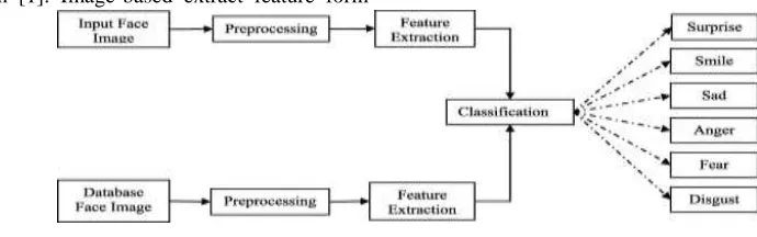
II. CONSTRUCTION OF AN IMAGE-BASED FER SYSTEM
The principal approaches (i.e., image-based and model based) to FER using static images are explained in [1]. Image-based extract feature form
the image without extensive knowledge about the object of interest, which are fast and simple. The model based methods attempt to recover the volumetric geometry of the scene, which are slow and complex [1]. Geometric features present the shape and location of facial components (including mouth, eyebrows, eyes and nose). The facial feature points or facial components are obtained from the feature vector that represents the face geometry.
Fig 1: System Level Diagram
The appearance feature can be taken from either the whole face or specific regions in a face image. This paper focused on the static color image and a holistic technique of the image-based method is used for feature extraction. Image based FER systems consist of several components or modules, including face detection and normalization, feature extraction, classification and feature selection. The system level diagram of FER system shown in Figure 1 The following section will describe briefly about YCbCr, CIELab, and CIELuv [13].
A. Face Detection and Normalization
In this module is to obtain face images, which have normalized intensity, are uniform in shape and size and depict only the face region. Face area of an image is detected using the Viola-Jones method based on the Haar-like features and the AdaBoost learning algorithm [14]. The Viola and Jones method is an object detection algorithm provides competitive object detection in the real-time. Features used by Viola and Jones are derived from pixels selected from rectangle area imposed over the picture and exhibit high sensitivity to the vertical and horizontal lines. After face detection the
image is scaled into some size (e.g.,64 × 64 pixels).
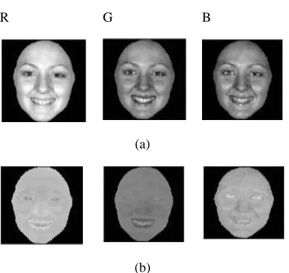
Color values in the face image are then normalized with respect to RGB values of the image.
Color normalization is used to reduce the lighting effect because the normalization process is actually a brightness elimination process. Input image
of 𝑁1× 𝑁2 pixels represented in the RGB color
space,
𝑋 = {𝑋𝑛3[𝑛
1, 𝑛2]│1 ≤ 𝑛1≤ 𝑁1, 1 ≤ 𝑛2≤ 𝑁2, 1 ≤
𝑛3≤ 3},
the normalized values, 𝑋𝑛𝑜𝑟𝑚
𝑛3
[𝑛1, 𝑛2], are defined by
𝑋𝑛𝑜𝑟𝑚 𝑛3
[𝑛1, 𝑛2] =
𝑋𝑛3[𝑛
1, 𝑛2]
∑ 𝑋𝑛3[𝑛
1, 𝑛2] 3
𝑛3=1
---(1)
where 𝑋𝑛𝑜𝑟𝑚𝑛3 [𝑛
1, 𝑛2] for 𝑛3= 1,2,3 corresponding to
red, green, and blue (or R, G, and B) components of the image X.
It is obvious that
∑ Xnorm
n3 [n
1, n2] = 1 3
n3=1
R G B
(a)
(b)
Fig 2: Facial expression images: (a) the original color components (b) the normalized color components.
B. Feature Extraction
Feature extraction have been studied and compared in terms of their performance, including
principal components analysis, independent
components analysis, linear discriminates analysis (LDA), the Gabor filter bank, etc. In [1] presents the Gabor filter has better performance than the rest. The Gabor filters model the receptive field profiles of cortical simple cells quite good [1], [15]. Gabor filter have two major drawbacks i.e., the maximum bandwidth of Gabor filter the maximum bandwidth is limited to approximately one octave, and the Gabor filter are not optimal to achieve broad spectral information with the maximum spatial localization [16]. The Gabor filter are band pass filters, which may suffers from loss of the low and the high-frequency information is reported in [17]. To overcome the bandwidth limitation of the traditional Gabor filter, Field proposed Log-Gabor filter [17]. Response of the Log-Gabor filter, is Gaussian when viewed on a logarithmic frequency scale instead of a linear. It allows more information to be capture in the high-frequency area with desirable high pass characteristics. A bank of 24 Log-Gabor filter is employed to extract the facial features. Polar form of 2-D Log-Gabor filters in frequency domain is given by
𝐻(𝑓, 𝜃) = 𝑒𝑥𝑝
{ − [ln(𝑓𝑓
0)] 2
2 [ln(𝜎𝑓𝑓
𝑜)] 2
}
𝑒𝑥𝑝 {−(𝜃 − 𝜃0)
2
2𝜎𝜃2
}
---(3)
where 𝐻(𝑓, 𝜃) is frequency response function of the
2-D Log-Gabor filter, f and 𝜃 denotes the frequency
2-D Log-Gabor filters, f and 𝜃 denotes the frequency
and the phase/angle of the filter.𝑓𝑜 is the filter center
frequency and 𝜃0 the filter's direction. The constant
𝜎𝑓 defines the radial bandwidth B in octaves and the
constant 𝜎𝜃 angular bandwidth ∆Ω in radians.
𝐵 = √ 2
𝑙𝑛2× |𝑙𝑛 ( 𝜎𝑓
𝑓0
)|
2
, ∆Ω= 2𝜎𝜃√
2 𝑙𝑛2
---(4)
In this paper describes here, the ratio 𝜎𝑓/𝑓0
is kept constant for varying𝑓0, B is set to one octave
and the angular bandwidth is set to one octave and
the angular bandwidth is set to ΔΩ=π/4 radians. 𝜎𝑓
is be determined for a varying value of𝑓0. Six scales
and four orientations are implemented to extract features from face images. It leads to 24 filter transfer
functions representing different scales and
orientations. Image filtering is performed in the frequency domain making the process faster compared with the special domain convolution. After 2-D fast Fourier transform (FFT) into the frequency domain, the image arrays, X, are changed into the spectral vectors X and multiplied by the log-Gabor
transfer functions {𝐻1, 𝐻2, … 𝐻24} producing 24
spectral representations for each image [17]. Spectra are then transformed block to the spatial domain via the 2-D inverse FFT. In this process results are obtained in the large numbers which are not suitable to build the robust learning models for classifications.
C. Feature Selection
selection and adopted to select the optimum features. As per the MIQ features selection if a feature vector has expression randomly or uniformly distributed in different classes and its MI with these classes is zero. If a feature vector is different from the other features for different classes, it will have large MI. Let F denotes the feature space; C denotes a set of
classes𝐶 = {𝑐1, 𝑐2, … , 𝑐𝑘}, and 𝑣𝑡 denotes the vector
of N observation for that feature.
𝑣𝑡= [𝜐𝑡1, 𝜐𝑡2, … , 𝜐𝑡𝑁]𝑇 ---(5)
where 𝑣𝑡 is an instance of the discrete random
variable 𝑉𝑡. The MI between features 𝑉𝑡 and 𝑉𝑠 is
given by
𝐼(𝑉𝑡; 𝑉𝑠) = ∑ ∑ 𝑝(𝑣𝑡, 𝑣𝑠)𝑙𝑜𝑔
𝑝(𝑣𝑡, 𝑣𝑠)
𝑝(𝑣𝑡)𝑝(𝑣𝑠)
𝑣𝑠∈𝑉𝑠
𝑣𝑡∈𝑉
---(6)
where 𝑝(𝑣𝑡, 𝑣𝑠) is the joint probability distribution
function (PDF) of 𝑉𝑡 and 𝑉𝑠, 𝑝(𝑣𝑡) and 𝑝(𝑣𝑠) are the
marginal PDFs of 𝑉𝑡 and 𝑉𝑠, for 1 ≤ 𝑡 ≤ 𝑁𝑓 ,1 ≤ 𝑠 ≤
𝑁𝑓, and 𝑁𝑓 is the input dimensionality, which equals
the number of features in the dataset. The Mi
between the 𝑉𝑡 and C can be represent by entropies
[19]
𝐼(𝑣𝑡; 𝐶) = 𝐻(𝐶) − 𝐻(𝐶׀𝑣𝑡) ---(7)
where
𝐻(𝐶) = − ∑ 𝑝(𝐶𝑖)
𝑘
𝑖=1
log(𝑝(𝐶𝑖))
---(8)
𝐻(𝐶│𝑉𝑡= − ∑ ∑ 𝑝(𝐶𝑖, 𝑣𝑡) log(𝑝(𝐶𝑖|𝑣𝑡)) 𝑣𝑡∈𝑉𝑡
𝑘
𝑖=1
---(9)
where H(C) is the entropy of C, 𝐻(𝐶│𝑉𝑡) is the
conditional entropy of C on 𝑉𝑡, and k is the numbers
of classes ( for six expression, 𝑘 = 6). The features
(𝑉𝑑) for desired feature subset, S, of the form (𝑆; 𝑐)
where 𝑆 ⊂ 𝐹 and 𝑐 ∈ 𝐶 is selected based on solution
of following problems:
𝑉𝑑= 𝑎𝑟𝑔 max
𝑉𝑡 {
𝐼(𝑉𝑡; 𝐶)
1
|𝑠|∑ 𝐼(𝑉𝑡; 𝑉𝑠)
} 𝑉𝑡∈ 𝑆̅, 𝑉𝑠∈ 𝑆
---(10)
where 𝑆̅ is the complement features subset of S, |𝑆| is
the number of features in subset S and 𝐼(𝑉𝑡; 𝑉𝑠) is the
MI between the candidate features (𝑉𝑡) and the
selected feature and intra-class features is maximized. MI between the selected feature and inter-class features is minimized. These features are used for emotion classification.
D. Classification
The LDA classifier was studied for the same database and provides the better result than other classifiers [5]. The selected features using the aforementioned MIQ techniques are classified by a multiclass LDA classifier. In [20] proposes a natural extension of Fisher linear discriminant that deals with more than two classes which uses multiple discriminant analysis. Projection from the high dimensional space to a low-dimensional space and the transformation descried to maximize the ratio of
inter-class scatter (𝑆𝑏) to the intra-class (𝑆𝑤) scatter.
The 𝑆𝑏 can be viewed as the sum of square of
distance between each class mean and the mean of all
training samples. 𝑆𝑤 can be regarded as the average
class-specific covariance. Intra-class (𝑆𝑤) and
inter-class (𝑆𝑏) matrices for feature vectors (𝑋𝑓) are given
by
𝑆𝑏 = ∑ 𝑚𝑖(𝑋𝜇𝑖 𝑓
− 𝑋𝜇 𝑓
)(𝑋𝜇𝑖 𝑓
− 𝑋𝜇 𝑓
)2
𝑁𝑐
𝑖=1
---(11)
𝑆𝑤= ∑ ∑ (𝑋𝑓− 𝑋𝜇𝑖
𝑓
)(𝑋𝑓− 𝑋
𝜇𝑖 𝑓
)𝑇
𝑋𝑓∈𝑐 𝑖
𝑁𝑐
𝑖=1
---(12)
where 𝑁𝑐 is the number of classes (i.e., for six
expression, 𝑁𝑐= 6), 𝑚𝑖 is the number of training
samples for each class. 𝑐𝑡 is the class label, 𝑋𝜇𝑖
𝑓 is the
mean vector for each class samples (𝑚𝑖), and 𝑋𝜇
the total mean vector over all training sample (m) defined by 𝑋𝜇𝑖 𝑓 = 1 𝑚𝑖∑ 𝑋 𝑓 𝑋𝑓∈𝐶
𝑖 ---(13)
𝑋𝜇 𝑓 = 1 𝑚∑ 𝑚𝑖𝑋𝜇𝑖 𝑓 𝑁𝑐
𝑖=1 ---(14)
After obtaining 𝑆𝑤 and 𝑆𝑏 based on Fisher's criterion
the linear transformation, 𝑊𝐿𝐷𝐴, can calculated by
solving the generalized Eigen value (𝜆) problem
𝑊𝐿𝐷𝐴𝑇 𝑆𝑏 = 𝜆𝑊𝐿𝐷𝐴𝑇 𝑆𝑤 ---(15)
The transformation 𝑊𝐿𝐷𝐴 is given the
classification can be performed in the transformed space based on preformed distance measure such as
the Euclidean distance, ‖•‖. The instance, 𝑋𝑛
𝑓 , is classified to
𝐶𝑛= 𝑎𝑟𝑔 min
𝑖 ‖𝑊𝐿𝐷𝐴𝑋𝑛 𝑓
− 𝑊𝐿𝐷𝐴𝑋𝜇𝑖
𝑓
‖ ---(16)
where 𝑐𝑛 denotes the predicted class-label for 𝑋𝑛
𝑓 and
𝑋𝑛 𝑓
is the centriod of the ith class.
III. COLOR SPACES
Several image representation models in the color space used for image processing [21]. The RGB color space is used in the image processing and pattern recognition systems. Color space can be used to generate the other alternative color formats
including: YCbCr, CIELab, and CIELuv. The YCbCr
color space is a ditial and offset version of the YUV used by the NTSC or the PAL television/video standard [13]. Conversion function between RGB and
YCbCr is defined by
[ 𝑌 𝑈 𝑉 ] = [ 65.481128.55324.966 −37.774 − 74.159111.934
111.958 − 93.751 − 18.207 ] [
𝑋𝑛𝑜𝑟𝑚1
𝑋𝑛𝑜𝑟𝑚2
𝑋𝑛𝑜𝑟𝑚2
] ---(17) [ 𝑌 𝐶𝑏 𝐶𝑟 ] = [ 16 128 128 ] + [ 𝑌 𝑈 𝑉
] ---(18)
where 𝑋𝑛𝑜𝑟𝑚
𝑛3 , 1 ≤ 𝑛
3≤ 3, is defined in the (1).
To Convert the PGB to perceptual color spaces (CIELab or CIELuv ), the RGB is first converted to XYZ color space, which than converted to perceptual color spaces. Components L are same for both CIELab and CIELuv color spaces. Conversion procedure is as follows in [13]
[ 𝑋 𝑌 𝑍 ] = [ 0.4310.3420.178 0.2220.7070.071 0.0200.1300.939 ] [ 𝑋𝑛𝑜𝑟𝑚1
𝑋𝑛𝑜𝑟𝑚2
𝑋𝑛𝑜𝑟𝑚3
] ---(19)
𝐿 =
{
116 × (𝑌
𝑌𝑛
)
1 3
− 16𝑌 𝑌𝑛
> 0.008856
903 × (𝑌
𝑌𝑛
),𝑌 𝑌𝑛
≤ 0.008856
---(20)
𝑎 = 500 × (𝑓 (𝑋
𝑋𝑛) − 𝑓 ( 𝑌
𝑌𝑛)) ---(21)
𝑏 = 200 × (𝑓 (𝑌
𝑌𝑛) − 𝑓 (
𝑍
𝑍𝑛)) ---(22)
where 𝑋𝑛, 𝑌𝑛, and 𝑍𝑛 are the reference white
tri-stimulus value which are defined in CIE chromaticity diagram [21] and
𝑓(𝑡) = {𝑡
1
3,𝑡 > 0.008856
7.787 × 𝑡 + 16
116, 𝑡 ≤ 0.008856
---(23)
for 𝑢 and 𝑣 color components, the conversion is
defined by
𝑢 = 13 × 𝐿 × (𝑢′− 𝑢𝑛′ )𝑣 = 13 × 𝐿 × (𝑣′− 𝑣𝑛′)
---(24)
The equation for 𝑣′ and 𝑢′ are given below
𝑢′= 4𝑋
𝑋+15𝑌+3𝑍 ---(25)
𝑣′= 9𝑌
The quantities 𝑢′𝑛 and 𝑣′𝑛 are the (𝑢′, 𝑣′) chromaticity coordinates of a specific white object defined by
𝑢′𝑛= 4𝑋𝑛
𝑋𝑛+15𝑌+3𝑍𝑣′𝑛=
9𝑌 𝑋𝑛+15𝑌𝑛+3𝑍
---(27)
IV. EXPERIMENTAL RESULTS
Fig 3: Training of the Dataset
Fig 4: Select Image from User
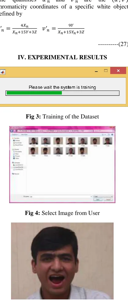
Fig 5: Input Image of Expression for Testing
Fig 6: Obtained result as surprise
V. CONCLUSION
Local Binary Pattern facial expression approach is proposed in this paper, the present is evaluated with the Indian face data base under different color transformations and resolution and it is shown that the CIE-Lab and CIE-LUV
transformation outperforms the highest
recognition rate and the proposed method is also compared against the conventional Gabor based approaches which fall short of more than 2 % in recognition rate .This work can be further extended with more frontal facial image data base for more accurate results.
REFERENCES
[1] B. Fasel and J. Luettin, “Automatic facial
expression analysis: A survey,”Pattern Recognit.,
vol. 36, no. 1, pp. 259–275, 2003.
[2] P. Ekman, E. T. Rolls, D. I. Perrett, and H. D. Ellis, “Facial expressions of emotion: An old
controversy and new findings discussion,” Phil.
Trans. Royal Soc. London Ser. B, Biol. Sci., vol. 335, no. 1273, pp. 63–69, 1992.
[3] A. Mehrabian, Nonverbal Communication.
London, U.K.: Aldine, 2007.
[4] M. Pantic and I. Patras, “Dynamics of facial expression: Recognition of facial actions and their temporal segments from face profile image
sequences,” IEEE Trans. Syst., Man, Cybern. B, vol.
36, no. 2, pp. 433– 449, Apr. 2006.
[5] J. Wang, L. Yin, X. Wei, and Y. Sun, “3-D facial expression recognition based on primitive surface
feature distribution,” in Proc. IEEE Conf. Comput.
Vis. Pattern Recognit., Jun. 2006, pp. 1399–1406. [6] Y. Lijun, C. Xiaochen, S. Yi, T. Worm, and M. Reale, “A high-resolution 3-D dynamic facial
Gesture Recognit., Amsterdam, The Netherlands, Sep. 2008, pp. 1–6.
[7] S. M. Lajevardi and Z. M. Hussain, “Emotion recognition from color facial images based on multilinear image analysis and Log-Gabor filters,” in
Proc. 25th Int. Conf. Imag. Vis. Comput., Queenstown, New Zealand, Dec. 2010, pp. 10–14. [8] L. Torres, J. Y. Reutter, and L. Lorente, “The importance of the color information in face
recognition,” in Proc. Int. Conf. Imag. Process., vol.
2. Kobe, Japan, Oct. 1999, pp. 627–631.
[9] P. Shih and C. Liu, “Comparative assessment of content-based face image retrieval in different color
spaces,” Int. J. Pattern Recognit. Artif. Intell., vol.
19, no. 7, pp. 873–893, 2005.
[10] Z. Liu and C. Liu, “A hybrid color and frequency features method for face recognition,”
IEEE Trans. Image Process., vol. 17, no. 10, pp. 1975– 1980, Oct. 2008.
[11] C. J. Young, R. Y. Man, and K. N. Plataniotis, “Color face recognition for degraded face images,”
IEEE Trans. Syst., Man, Cybern. B, Cybern., vol. 39, no. 5, pp. 1217–1230, Oct. 2009.
[12] M. Corbalán, M. S. Millán, and M. J. Yzuel, “Color pattern recognition with CIELab coordinates,”
Opt. Eng., vol. 41, no. 1, pp. 130–138, 2002.
[13] G. Wyszecki and W. Stiles, Color Science:
Concepts and Methods, Quantitative Data, and Formulae (Wiley Classics Library). New York: Wiley, 2000.