SIMULATION AND OPTIMISATION OF A DRYING MODEL FOR A FORCED CONVECTION GRAIN DRYER
BOOKER ONYANGO OSODO
A Thesis Submitted in Partial Fulfillment of the Requirements for the Award of the Degree of Doctor of Philosophy (Renewable Energy Technology) in the
Department of Energy Technology in the School of Engineering and Technology of Kenyatta University
ii
DECLARATION
This thesis is my original work and has not been presented for award of any diploma or degree in any other University.
Signature ………Date ………
BOOKER ONYANGO OSODO (REG NO: J98/25749/2011)
This thesis has been submitted for examination with our approval as the University supervisors.
Signature ………Date ………
Prof. Daudi M. Nyaanga
Associate Professor, Department of Agricultural Engineering, Egerton University
Signature ………Date ………
Dr. Jeremiah K. Kiplagat
iii
DEDICATION
iv
ACKNOWLEDGEMENT
v
TABLE OF CONTENTS
DECLARATION ... ii
DEDICATION ... iii
ACKNOWLEDGEMENT ... iv
TABLE OF CONTENTS ... v
LIST OF FIGURES ... ix
LIST OF SYMBOLS / ACRONYMS ... xi
ABSTRACT ... xiv
CHAPTER ONE: INTRODUCTION ... 1
1.1 Background ... 1
1.2 Statement of the Problem ... 4
1.3 Justification ... 4
1.4 Objectives of the Study ... 5
1.5 Research Questions ... 5
1.6 Scope and Limitations ... 5
CHAPTER TWO: LITERATURE REVIEW ... 7
2.1 Solar Crop Drying ... 7
2.1.1 Solar thermal collectors ... 7
2.1.2 Types of solar dryers ... 9
2.1.3 Drying theory ... 14
2.2 Airflow Simulation and Sizing of Dryer ... 16
2.2.1 Simulation ... 18
2.2.2 Pressure drop and fan sizing ... 19
2.3 Effect of Various Factors on Dryer Performance ... 22
2.3.1 Effect of air velocity ... 24
2.3.2 Effect of grain layer thickness ... 26
2.3.3 Effect of number of trays ... 26
2.3.4 Effect of drying air temperature ... 27
2.4 Theoretical Framework... 27
2.4.1 Optimisation of dryer performance ... 27
vi
2.5 Past studies on selection of drying models ... 36
2.6 Observations from Literature Review ... 40
CHAPTER THREE: MATERIALS AND METHODS ... 41
3.1 Research Site ... 41
3.2 Simulation and Sizing of Experimental Dryer ... 41
3.2.1 Simulation to estimate grain layer thickness and number of trays ... 41
3.2.2 Sizing of solar dryer ... 44
3.3 Effect of Selected Parameters on Dryer Performance ... 45
3.3.1 Efficiency, moisture content and removal rate... 50
3.3.2 Air velocity and grain layer thickness ... 52
3.3.3 Number of trays ... 53
3.3.4 Drying air temperature ... 53
3.3.5 Relative Humidity ... 54
3.4 Optimisation and Verification of Selected Drying Model... 54
3.4.1 Optimisation of dryer performance ... 54
3.4.2 Testing and verification of drying model ... 59
CHAPTER FOUR: RESULTS AND DISCUSSION ... 62
4.1 Simulation and Sizing of Experimental Dryer……….62
4.1.1 Grain layer thickness and number of trays ... 62
4.1.2 Sizing of solar dryer ... 63
4.1.3 Simulation of air flow through experimental dryer ... 65
4.2 Effect of Selected Parameters on Performance of Experimental Dryer ... 66
4.2.1 Air velocity and grain layer thickness ... 70
4.2.2 Number of trays ... 75
4.2.3 Drying air temperature ... 77
4.2.4 Relative humidity ... 80
4.3 Optimum Dryer Performance and Selected Drying Model ... 81
4.3.1 Optimum dryer performance ... 81
4.3.2 Tested and Verified Drying Model ... 88
CHAPTER FIVE: CONCLUSIONS AND RECOMMENDATIONS ... 94
5.1 Conclusions ... 94
vii
REFERENCES ... 96
APPENDIX I: SIMULATION AND SIZING ... 107
APPENDIX II: EFFECTS ON DRYER PERFORMANCE ... 114
APPENDIX III: OPTIMISATION AND MODELING ... 118
APPENDIX IV: MOISTURE CONTENT DATA ... 135
APPENDIX V: ENGINEERING DRAWINGS OF SOLAR DRYER ... 137
viii
LIST OF TABLES
Table 2. 1: Mathematical Models for Drying Curves ... 33
Table 2. 2: Drying Models with Model Constants for Maize ... 37
Table 2. 3: Fitting Different Products to Various Drying Models ... 39
Table 3. 1: Dryer Performance Parameters and their Levels ... 55
Table 4. 1: Dryer Performance for One and Two Trays ... 76
Table 4. 2: Effect of Temperature on Drying Efficiency (Turkey Method) ... 80
Table 4. 3: Effect of Temperature on Moisture Removal Rate (Turkey Method) ... 80
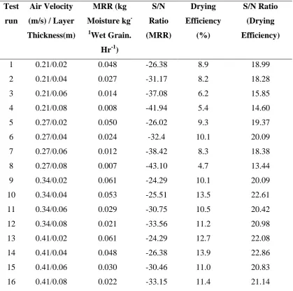
Table 4. 4: Moisture Removal Rates & SN Ratios ... 82
Table 4. 5: Mean SN Ratios for Moisture Removal Rate ... 83
Table 4. 6: Mean SN Ratios for Drying Efficiency ... 84
Table 4. 7: Effects of Air Velocity on MRR and Drying Efficiency ... 85
Table 4. 8: Effect of Grain Layer Thickness on MRR and Drying Efficiency ... 86
Table 4. 9: , R2 & RMSE for Different Models ... 89
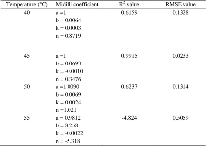
Table 4. 10: Midilli Coefficients and Goodness of Fit Values ... 89
Table 4. 11: Predicted and Experimental Moisture Ratios at Different Temperatures ... 90
ix
LIST OF FIGURE
Figure 2. 1: Natural Convection Solar Drier ... 11
Figure 2. 2: Active Solar Drier 1 ... 12
Figure 2. 3: Direct Solar Dryer ... 13
Figure 3. 1: Model creation ... 43
Figure 3. 2: Flow chart of preprocessing stage of simulation ... 43
Figure 3. 3: Post-processing stage of simulation ... 44
Figure 3. 4: Schematic Diagram of solar grain dryer ... 49
Figure 3. 5: Schematic Diagram of electrically heated grain dryer ... 50
Figure 3. 6: Taguchi optimisation procedure (Minitab 17 Statistical software) ... 57
Figure 3. 7: Flow Chart for Computer Simulation Model ... 61
Figure 4. 1: Variation of Pressure for a Single Layer of Thickness 0.1 m ... 64
Figure 4. 2: Side view of Solar Dryer ... 65
Figure 4. 3: Simulated Air Flow through Drying Cabinet ... 66
Figure 4. 4: Temperature Variation for Unloaded Dryer... 67
Figure 4. 5: Variation of Solar Radiation with Time for Unloaded Dryer ... 68
Figure 4. 6: Temperature variation for dryer loaded with grain ... 69
Figure 4. 7: Temperature variation (including grain surface temperature) ... 70
Figure 4. 8: Drying Efficiency vs Air Velocity ... 71
Figure 4. 9: Moisture Removal Rate vs. Air Velocity ... 72
Figure 4. 10: Drying Efficiency vs Grain Layer Thickness ... 74
Figure 4. 11: Moisture Removal Rate vs. Grain Layer Thickness ... 75
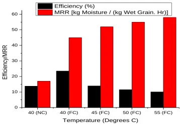
Figure 4. 12: Effect of Temperature on Dryer Performance ... 77
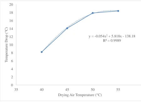
Figure 4. 13: Temperature drop within grain Layer ... 79
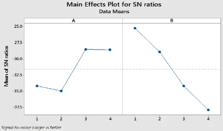
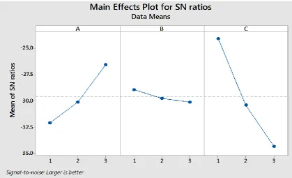
Figure 4. 14: Main effects Plot for MRR during Solar Frying ... 83
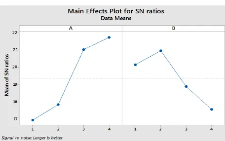
Figure 4. 15: Main Effects Plot for Drying Efficiency during Solar Drying... 84
Figure 4. 16: Main Effects Plot for MRR during Laboratory Drying ... 87
Figure 4. 17: Main Effects Plot for Drying Efficiency during Laboratory Drying .. 87
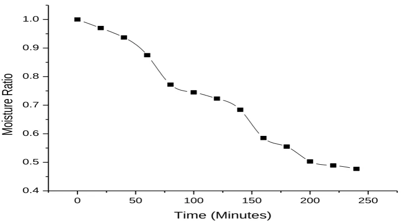
Figure 4. 18: Variation of Moisture Ratio with time ... 88
Figure 4. 19: Predicted vs Experimental Moisture Ratios ... 92
Figure 4. 20: Curves for Predicted and Experimental Moisture Ratio at 40 °C ... 92
x
LIST OF PLATES
xi
LIST OF SYMBOLS / ACRONYMS
A Area
Ac Collector area
cpa Specific heat capacity of air
dp Particle Diameter
E Energy
Hv Latent Heat of Vaporisation
Lp Length of Bed
P Rate of Permeation
Pf Fan power
ΔP Pressure Drop
Mass Flow rate
ma Mass of drying air
mw Mass of moisture evaporated
Q Volume Flow Rate
T Temperature of air
Td,o Air temperature at dryer outlet (K)
Td,i Air temperature at dryer inlet
Ig Rate of total radiation incident on the absorber surface
Drying rate at any time E Energy consumed by dryer X Moisture content of wet material Xr Moisture Ratio
Initial moisture content
Equilibrium moisture content
Critical moisture content
MRR Moisture Removal Rate OSD Open sun drying
xii EUR Energy Utilisation Ratio
HVAC Heating Ventilation and Air Conditioning
MS Mild steel
xiii
GREEK SYMBOLS Viscosity of Fluid (Drying Air)
uo Fluid Superficial Velocity
ɛ Void Space of Bed ρ Density of drying Air Efficiency
Subscripts
A Air
c Collector cb Drying cabinet d dryer
xiv
ABSTRACT
1
CHAPTER ONE: INTRODUCTION 1.1 Background
Food security of a nation is basic to the well-being of the nation’s people, since access to quality, nutritious food is fundamental to human existence (USDA, 2018). However, a large proportion of food product is often lost between harvesting and consumption. The problem of food loss is particularly significant in developing countries. In these countries, food losses are estimated to be of the order of 40%, but can rise to be as high as 80% under very adverse conditions. A significant percentage of these losses is related to improper and or untimely drying of foodstuffs such as cereal grains, meat, tubers and fish (Bolaji and Olalusi, 2008). One reason for loss of grain after harvesting is spoilage resulting from high moisture content. Postharvest loss of maize in Kenya in 2007 was 21.1% (Hodges, 2009). Drying of the grain is necessary to avoid loss between harvesting and consumption. Moist and partly moist crop is prone to fungus infection, which renders it unusable. High moisture content also encourages loss due to attacks by insects, pests and increased respiration (Tiwari, 2002; Twidell and Weir, 2006). According to Barawal and Tiwari (2008), drying of crop helps to achieve better product quality, longer safe storage and reduction of post-harvest loss hence ensuring more food is available for the growing world population. Also, drying using solar energy leads to conservation of conventional energy sources.
Grain drying may be carried out using different sources of energy. However, solar energy is preferred to other alternative sources of energy such as wind and shale since it is abundant and freely available, inexhaustible and non-polluting (Akinona
2
foreign materials such as dust, insects and micro-organisms are other problems associated with open sun drying (Tiwari, 2002; Tiwari, 2016). In addition, it results in loss of quality (Sharma and Wadhawan, 2018).
Other modes of grain drying are direct solar drying otherwise known as cabinet drying, and indirect solar drying. Direct solar drying utilizes the greenhouse effect to dry crop placed in an enclosure covered with a transparent cover, the crop being directly exposed to solar radiation. This mode of drying is, however limited to small scale applications due to its small capacity. The crop is also prone to discoloration due to direct exposure to solar radiation. Moisture condensation inside the glass cover reduces the transitivity of the glass. Some of the limitations of direct solar dryers are addressed by indirect solar dryers, in which heated air from a separate solar collector is passed through the crop, placed in a separate chamber (Tiwari, 2002). A mixed mode solar dryer utilises hot air from the solar collector, but at the same time the drying chamber absorbs energy directly through transparent walls and roof (Bolaji and Olalusi, 2008). According to Simate (2003), for the same quantity of grain dried, the mixed mode solar dryer is shorter in length than the indirect mode dryer, resulting in savings in construction material. This is because it receives extra energy through drying chamber transparent cover, reducing on energy demand from the collector. The drying cost in the mixed mode solar dryer is 26% lower than for indirect mode dryer. Also, there is more uniform moisture content distribution due to the additional drying from the direct radiation at the grain bed.
3
Convection Dryer (Sharma and Wadhawan, 2018). The performance of a dryer may also be evaluated based on other criteria such as drying and dryer efficiency, uniformity of drying and quality of final product (extent of cracking and discoloration of grain) as well as total drying time (Mohanraj and Chandrasekar, 2009; Kassem et al., 2011).
Good performance of a dryer leads to desirable properties of dried product, such as low and uniform moisture content, minimal proportion of broken or damaged grain, low mold count and high nutritive value. High dryer efficiency is also desirable (Tiwari, 2016). The process of optimisation may be used to manipulate parameters that affect dryer performance characteristics, so that a combination of parameter levels that result in minimum or maximum performance measures, whichever is desired is determined. According to Sevik (2013) and Alqadhi et al. (2017), factors affecting drying rate include air temperature and velocity, product type, layer thickness and moisture content of product, method of drying, moisture diffusivity and drying kiln structure. Others are crop porosity and humidity of the surrounding air. The surface area of the crop exposed is yet another factor that affects drying rate (Twidell and Weir, 2006; Bolaji and Olalusi, 2008). Efficiency of a dryer, however, is affected by air flow rate and drying air temperature (Aissa et al., 2014; Balbine et al., 2015).
Simulation, which is the imitation or reproduction of the behavior of a system or process (Frangopoulos and Sciubba, 2002), is useful in the design, as it saves on the time and resources that would otherwise be required to obtain optimal performance. Modelling of solar drying curves involves describing variation of moisture ratio as a function of drying time (Kamenan et al., 2009) and various researchers have developed different such drying models for a variety of products. According to Eterkin and Firat (2015), various statistical tools, such as Coefficient of Determination (R2), Root Mean Square Error (RMSE), Modelling Efficiency (EF), Root Mean Square Deviation (RMSD), Reduced Chi Square ( ) may be used to
4 1.2 Statement of the Problem
Forced convection solar dryers achieve greater drying rates than natural convection dryers (Harun et al., 2016). However, their performance is often not optimal. One reason for this is inadequate distribution of air flow, resulting in inadequate drying air in some sections of the dryer and hence uneven drying of the grain. Sometimes, the fan is undersized, leading to insufficient air flow (and velocity), or oversized, leading to excessive energy consumption and in extreme cases grain being blown upward. Also use of inappropriate grain layer thickness leads to poor performance. If the grain layer is too thick, some sections do not dry uniformly as they receive air which is saturated with moisture. If too thin, air exits while still having capacity to remove moisture, leading to low thermal efficiency. Very high air flow rates do not give the air enough time to absorb moisture, and may lead to low thermal efficiency while very low flow rates lead to low drying rate. Non-optimal layer thickness and air flow rate leads to poor dryer performance on the basis of drying efficiency, moisture removal rate and total drying time. Inability to predict drying time for different initial grain moisture content makes it impossible to plan drying schedules. Design of dryers that meet these criteria, without use of simulation, would require troublesome development stages, involving iterations and continued testing and use of prototypes, a process which would be expensive and time consuming.
1.3 Justification
5
The ability to predict drying time is of essence to the farmer, and will enable the farmer to plan a drying schedule. This is enabled by the computer simulation model developed as a result of the research.
1.4 Objectives of the Study
The broad objective of this research was to simulate, optimise and select a drying model for an experimental forced convection grain dryer.
The specific objectives were:
1. To simulate the grain quantity, fan and solar collector sizes for an experimental forced convection grain dryer
2. To establish the effect of air velocity, grain layer thickness, number of trays and drying air temperature on the performance of an experimental forced convection grain dryer
3. To optimise the performance of an experimental forced convection grain dryer and verify a selected drying model for it
1.5 Research Questions
1. What are the simulated grain quantities, fan and solar collector sizes for the experimental forced convection grain dryer?
2. How do air velocity, grain layer thickness, number of trays and drying air temperature affect the performance of the experimental forced convection grain dryer?
3. What is the optimal combination of drying air velocity, temperature and grain layer thickness that should be used for the grain dryer and which drying model best describes the drying curve it?
1.6 Scope and Limitations
6
7
CHAPTER TWO: LITERATURE REVIEW
This chapter outlines literature on crop drying, especially the application of solar energy in the grain drying process. It reviews the application of simulation in the development and optimisation of a forced convection solar grain dryer as well as selection and fitting of various drying models for different products.
2.1 Solar Crop Drying
A great proportion of crop is often lost between harvesting and consumption. The problem of post-harvest loss is particularly significant in developing countries. In these countries, these losses are estimated to be of the order of 40%, but can rise to be as high as 80% under very adverse conditions (Bolaji and Olalusi, 2008). According to Adebayo et al. (2014) loss of crop occurs in the field (15%), during harvesting (13-20%), as well as during processing and storage (15-25%). Post-harvest loss of crop may be attributed to different causes. Pests, such as large grain borer account for 10-20% loss, while 5-10% of the losses may be attributed to poor storage facilities. Diseases, on the other hand, contribute to 5% of post-harvest crop loss (Bett and Nguyo, 2007). Also, a significant percentage of the losses is related to improper or untimely drying of foodstuffs such as cereal grains, meat, tubers and fish (Bolaji and Olalusi, 2008). Incidences of post-harvest product loss in Kenya have been estimated at 30%, and can rise to be as high as 100% with the advent of afflotoxin (Irungu, 2010). Maize is usually harvested with moisture content of between 18 % and 24 %. Drying maize to below 13.5% moisture content increases storage life and maintains quality by decreasing growth of fungi and insect infestation during storage. It also prevents germination (FAO, 1998; Irungu, 2010).
2.1.1 Solar thermal collectors
8
on two factors: the extent to which solar radiation is converted to heat, and the extent of heat losses to the surroundings (Klaus et al., 2014).
Solar collectors are classified into three categories: uncovered, covered and vacuum collectors. Uncovered collectors have no transparent cover hence the radiation is directly incident on the absorber surface. Reflection losses are minimized due to absence of reflective cover. Covered collectors have a transparent covering material, providing extra insulation, but there is also increase in reflective losses. In vacuum collectors, also called Evacuated Tube Solar Collectors (ETSCs), the absorber is encapsulated in vacuum tubes hence there is little loss to the surroundings. They can therefore be used for high temperature applications. Another way of classifying solar collectors is according to their shape, hence flat plate and concentrating collectors. Flat plate collectors have flat absorbers, and can deliver moderate temperatures, up to around 100 . Concentrating collectors have their performance optimized by
decreasing the area of heat loss. An optical device with a smaller area is placed between the source of radiation and the absorber. They find use in higher temperature applications (Klaus et al., 2014).
In a solar air heater, air is circulated in contact with a black radiation-absorbing surface, above which there is usually one or more transparent covers to reduce heat loss. Although solar air heaters come in various forms, a typical one consists of an absorbing plate, a rear plate with insulation below it, and the transparent cover on the exposed side. The air may flow above, below or both above and below the absorber plate. The absorber plate may be flat, corrugated (with rounded or v-troughs), finned or of the matrix type. In the matrix type, an absorbing matrix is placed in the air flow path between the glazing and the absorber plate. Another type of absorber plate is the overlapped transparent plate type, composed of a staggered array of partially blackened transparent plates. The transpiration collector, also called porous bed collector, is a variation of the matrix type, in which the matrix is closely packed, and the back absorber plate is eliminated (Garg and Prakash, 2005).
9
convection heat losses by removing air between the absorber and the glass cover, leaving radiation as the only remaining mechanism for heat loss. Because it is difficult to maintain vacuum in a flat plate collector, Evacuated Tube Solar Collectors (ETSC) were invented. Umayal et al. (2013) reported that evacuated tube solar collectors have many advantages over the flat plate collectors mostly used in solar dryers. These include high efficiency in performance as well as ability to perform even in bad weather. Dabra et al. (2013) noted that the performance of a vacuum tube collector was better than for a flat plate collector and was independent of climatic conditions. Reflectors may be used to enhance the efficiency of a solar collector. Maiti et al. (2011), while investigating an indirect solar dryer utilised for drying wet papads, showed that use of reflectors enhanced collector efficiency from 40 % to 58.5 %.
A flat plate collector was applied in this research due to the relatively low temperature requirement of 60 °C and also the abundance of solar energy in the region of the research. For such a collector, solar collector area Ac may be
determined from eq. (2.1), used by Dabra et al. (2013) and Aduewa et al. (2014).
c a o pa a CI
T
T
c
m
A
.)
(
(2.1)In the equation, and cpa represented mass flow rate and specific heat capacity of
air respectively, while and stood for maximum insolation on collector surface and solar collector efficiency, also respectively. To and Ta were used to represent
optimum dryer temperature and inlet temperature at ambient.
2.1.2 Types of solar dryers
10
other sources of energy since it is abundant, inexhaustible and non-polluting. This makes the use of solar dryers a more attractive option in crop drying (Akinona et al., 2006).
Drying using solar energy may be carried out by simply placing the crop in the open where it is exposed to radiation from the sun, in a process called Open Sun drying (OSD). Traditionally, grains have always been dried by OSD (Sodha et al., 1985). In OSD, however, there is considerable loss of the grain due to rodents, birds, insects and micro-organisms. Unexpected rain may result in increasing the moisture in the grain. Other problems encountered in OSD are discolouration due to ultra-violet radiation, as well as contamination by dust, dirt, insects and micro-organisms. There may also be over drying or insufficient drying (Tiwari, 2002).
11
Figure 2. 1: Natural Convection Solar Drier Source: Tiwari (2016)
12
evaporation of moisture. Sallam et al. (2013) compared drying of mint in two identical prototype solar dryers used under natural and forced convection modes. For the forced convection mode, a 0.75 kW fan was used and air entered the dryer at an inlet velocity of 4.2 m/s. This air velocity was rather high, in the light of findings by Sevik et al. (2013) who suggested that drying rate would not be influenced by air velocities above 4.2 m/s. They, however, reported that drying rates were higher for forced convection than for natural convection drying, findings similar to those of Jangai et al. (2009) and Ikejiofor (2010).
Figure 2. 2: Active Solar Drier 1 Source: Tiwari (2016)
Three distinct subclasses of passive or active solar drying systems can be identified, depending on the design arrangement of the system components and the mode of utilization of solar heat. These are: Integral or direct solar dryers, distributed or indirect solar dryers and mixed mode solar dryers (Weiss and Buchinger, 2012; Gregoire, 2009).
13
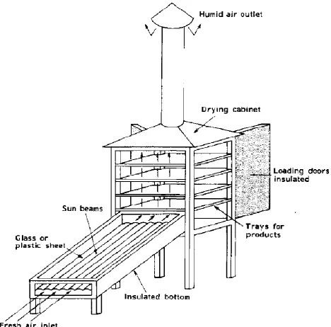
of the incident solar radiation is reflected back into the atmosphere by the glass cover, while the rest is transmitted through the glass onto the crop. The crop temperature is raised by the radiation incident on it, and it starts emitting long wavelength radiation, which unlike for OSD, is prevented from escaping into the atmosphere by the glass cover. As a result, the temperature in the chamber above the crop rises. The glass cover also prevents heat loss to the ambient by convection, thereby further increasing the temperature of the crop and chamber. As for OSD, the crop loses water by evaporation. Air entering into the chamber from below and exiting at the top takes away the moisture by natural convection as in passive dryers, or by forced convection, in the case of active dryers. Limitations of direct solar dryers include:
a) Small capacity limiting it to small scale applications
b) Discoloration of the crop due to direct exposure to solar radiation c) Moisture condensation inside the glass cover reducing its transitivity
d) Insufficient rise in crop temperature affecting moisture removal (Tiwari, 2002).
Figure 2. 3: Direct Solar Dryer Source: Tiwari (2016)
14
Instead, heated air from a separate solar collector is passed through the crop, placed in a separate chamber. Evaporation of moisture from the crop is obtained as in OSD and DSD (Tiwari, 2002).
In a mixed mode solar dryer, heated air from a separate solar collector is passed through a grain bed and at the same time the drying cabinet absorbs solar energy directly through a transparent wall and roof (Bolaji and Olalusi, 2008). Because solar dryers are not functional at night or during rainy or cloudy conditions, studies have been carried out to integrate them with back up heaters or heat storage systems. Kaaya and Kyamuhangire (2010) as well as Rigit et al. (2013) showed that use of biomass back up burners not only reduces drying time, but also improves quality of product.
This research adopted an indirect mode of forced convection solar drying. This was to ensure cracking and discoloration of grain, common in the direct mode was prevented. Application of a fan also made it possible to vary air flow rate to investigate how this affected the drying process.
2.1.3 Drying theory
The drying of grain occurs as water at the surface evaporates and water in the inner part migrates to the surface to also get evaporated. If left for long enough, a moist grain will give up water to the surrounding air until the grain reaches its equilibrium moisture content. Much of the moisture present in the crop is ‘free water’, loosely
held in the cell pores and is therefore quickly lost after harvest. The remaining water (usually 30-40%) is bound to the cell walls by hydrogen bonds, and is therefore harder to remove. Unsaturated air passing over the grain takes up water from it by evaporation, the heat to evaporate the water being derived from the air and the crop (Twidell and Weir, 2006; Bolaji and Olalusi, 2008).
15
different times. The diffusion theory relies on Fick’s law [eq. (2.2)] to explain liquid diffusion within the kernel. In this equation, P is the rate of permeation while k, A
and represent diffusion constant, cross sectional area and concentration gradient
respectively.
(2.2)
16
because one product was investigated, in which pore sizes and distribution could be assumed to be similar.
Kamenan et al. (2009), while analysing drying rate curve for cassava and plantain banana, showed the existence of two distinct phases: a constant drying rate phase and a falling drying rate phase. The constant drying rate phase, which is short and not available for all products, involves rise in temperature of the product up to attaining the wet bulb temperature characteristic of the drying environment. It is not taken into account during the analysis of the drying rate curve but describes a rapid movement of free water by capillarity from inside the product to the surface. In this phase, drying does not depend on the nature of the product. It only depends on the drying conditions, the moisture content tending towards the critical moisture content development.
The falling drying rate phase is further subdivided into two: the falling drying rapid rate phase and the falling drying slow rate phase. Once the moisture content is below the critical moisture level, capillary forces are not sufficient to transport moisture to the surface of the product. At the beginning of the falling drying rate phase, drying rate reduces rapidly. The zone of evaporation is now inside the product and there exist two sections with different modes of transport. Upstream in the centre of the product, there is still migration of water by capillarity. Downstream, migration is due to the diffusion phenomenon, in the case of vapour, and diffusion sorption, in the case of tied water. The moisture content now tends towards its level at hygroscopic equilibrium. The falling drying slow rate phase begins once the product is in the hygroscopic domain. During this phase, a resistance to vapour diffusion appears and if the temperature continues to rise, the first fissures in the product may appear (Kamenan et al., 2009).
2.2 Airflow Simulation and Sizing of Dryer
17
research, airflow through the dryer was simulated in order to ensure it would be well distributed within the drying chamber for uniform drying of the grain. . Also, the air must be able to penetrate the grain layers for drying to occur. This can be effected by ensuring the grain layers are not too thick, and that the number of grain layers is not too many for the air to penetrate. A fan that is able to overcome the static resistance to air flow also needs to be selected. According to Misha et al. (2013), uneven drying is the consequence of poor air flow distribution in the drying chamber. Product closer to the air inlet is better dried than that further, due to reduced temperature and air velocity. Actual measurement of air flow parameters is not only expensive and time consuming, but is also difficult since sensors have to be installed in many different positions. Simulation is a better option to apply in the investigation of air flow in a dryer. Simulating air flow within the drying cabinet can be used to ensure the design enhances air distribution. This would reduce or eliminate non-uniformity in drying, thereby increasing dryer efficiency. It may also be applied for predicting the pressure drop within the drying chamber, and use it to size the fan.
18 2.2.1 Simulation
Simulation deals with two systems. The first is the physical system, whose performance is to be studied, or whose design is to be optimized. The physical system may be a real system that is actually in operation, or it may only be on paper, and still at the design stage. The second system involved in simulation is a model of the system to be studied. The model may itself be another physical system, or it may be a mathematical model. Usually, simulation involves first, creation of a mathematical model of the system to be studied. This is followed, whenever possible, by manipulation of the model to obtain desired information. A computer is then used as another system to simulate the mathematical model. Then starting from the model, a second physical system is created (Frangopoulos and Sciubba, 2002). This process is summarized in Figure 2.4. Solar drying is, according to Garg and Prakash (2005), a complex phenomenon, depending on several parameters. Simulation models are greatly useful in predicting and studying inter-relationships between various parameters that affect the solar drying process.
Simulation soft wares come in different forms. Analysis Systems (ANSYS) software is a general purpose finite element modeling package for numerically solving a wide range of mechanical problems in areas such as heat transfer, fluid mechanics, static and dynamic structural analysis. It allows the construction of computer models of structures, components or systems, application of operating loads and other design criteria and study of parameters such as temperature distributions, air velocity and pressure. It permits an evaluation of a design without having multiple prototypes in testing (Nakasone et al., 2006).
19
ANSYS. First is by means of the Graphical User Interface (GUI), which uses conventions of popular Windows and X-Windows based programs. The second method uses command files (Nakasone et al., 2006). Li et al. (2015) used ANSYS to simulate air flow in a mixed flow grain dryer in order to determine how air velocity was influenced by air duct size. They found that smaller air ducts yielded higher air velocities.
Transient Systems (TRNSYS) uses a graphically based software environment to simulate the behavior of transient systems. It is made up of two parts. The first part is the engine, called the kernel. It reads and processes the input files, iteratively solves the system, determines convergence and plots the system variables. The second part is an extensive library of components, each of which models the performance of one part of the system. Models in the library include pumps, wind turbines and basic HVAC equipment, among approximately 150 other models in a standard library (University of Wisconsin, 2013). Habtamu (2008) used TRNSYS to simulate a cereal solar dryer and was able to predict useful energy and collector output temperatures for given incident flux, ambient air temperature and solar collector parameters. However, these predictions were not verified experimentally.
ComsolMultiphysics software is a general purpose software platform based on advanced numerical methods and is used for modeling and simulating Physics based problems. It is suitable for electrical, mechanical, fluid flow and chemical applications, among others. In addition, the user is able to include own equations that may describe a material property, boundary, source or even a unique set of partial differential equations. The user can then create new physics interphases from the equations entered (Comsol, 2012).
2.2.2 Pressure drop and fan sizing a) Pressure drop
Jia et al. (2009) explain that air flow through packed material may be described using the Ergun equation (eq. 2.3). According to this equation, pressure drop ,
20
viscosity ( void space ( and fluid density ( The effect of cross sectional area
(due to container diameter) is ignored in this equation.
(2.3)
Although there are many channels through packed material, fluid will normally only flow through a few of them, a phenomenon called channeling. This leads to lack of distribution of fluid flow. Another limitation is that of formation of hot spots, which leads to damage to the bed and packing materials (Sachdeva et al., 2012). The pressure drop in the drying chamber limits the number of trays that may be used. Due to high resistance to air flow through drying product, only a few drying shelves can be used without significantly affecting air movement (Aissa et al., 2014).
Jia et al. (2009) used glass beads and copper coated metal balls and air velocities ranging between 1 m/s – 4 m/s to study pressure drops through packed material and found that experimental data were within 20 % of the values predicted using Ergun equation. This equation was used in this research to simulate airflow up the dryer with grain as the packed material in an attempt to predict the pressure drop. Although the packed material was not grain, the air velocities used in the current research were within the range investigated by Jia et al. (2009).
b) Fan sizing
21
Typical air flow rates range from 0.25-0.51 m3/s.m2 of perforated screen area, these flow rates creating relatively low static pressures of 0.249-1.25 kPa in cross flow and mixed-flow dryers. The fan to be used for such a dryer must be of sufficient capacity to overcome this static pressure, being the resistive force the fan works against while trying to push the air through the grain column (Maier and Bakker-Arkema, 2002).
Fan power ( may be obtained either from manufacturers’ charts or from eqs. (2.4)
and (2.5), as suggested by Wilcke and Morey (2015) and Maier and Bakker-Arkema (2002).
(2.4)
(2.5)
( is air volume flow rate while Ps represents static pressure)
The equations are similar, although for eq. (2.5), an impeller efficiency of 60% has been assumed and incorporated. According to Weiss and Buchinger (2012), fan efficiency ranges between 30 % and 70 %, hence the assumption is reasonable to cater for most fans if cost of fan and that of power is the major consideration. In the current study, eq. 2.5 was adopted to cater for a general situation where efficiency of fan does not have to be used every time.
22
2.3 Effect of Various Factors on Dryer Performance
Various researchers have evaluated the performance of solar dryers on the basis of different criteria. Mohanraj and Chandrasekar (2009) use dryer thermal efficiency, drying rate and specific moisture extraction rate as their basis, while Kassem et al.
(2011) base their evaluation solely on dryer efficiency. Uniformity of drying in different trays, and even within the same tray, is also important in evaluating dryer performance. Drying time within a permissible maximum temperature so as not to cause loss in flavour, colour, aroma and vitamins is another measure (Murthy, 2009).
This research focused on drying rate and efficiency of dryer as performance criteria, these being factors that would interest the user.
Drying rate is given by eq. (2.6) [Twidell and Weir, 2006], and being
initial and final moisture fractions, respectively during a drying time t.
(2.6)
However, drying rate varies every instant and would not be beneficial to the user, in planning drying schedules, for example. This research therefore adopted moisture removal rate (ratio of mass of moisture removed to mass of wet grain per hour) as this would then be used to predict the total drying time for some given quantity of product with certain moisture content.
Factors affecting drying rate include air temperature, air velocity, porosity of product, layer thickness and moisture content of product. Other factors are humidity of the surrounding air, method of drying, moisture diffusivity and drying kiln structure (Twidell and Weir, 2006; Bolaji and Olalusi, 2008; Sevik, 2013). The total energy required to dry a given quantity of material may be estimated using eq. (2.7), the basic energy balance equation for the evaporation of water (Twidell and Weir, 2006; Bolaji and Olalusi, 2008).
23
In this equation, and represent mass of air through dryer and of water
vapour evaporated, respectively. and are the latent heat of vapourisation for
water and specific heat capacity of air, while and represent initial and final air
temperatures, also respectively
Different researchers have used different criteria and equations to determine efficiency of dryers. Average dryer thermal efficiency , applied by Aduewa et al. (2014) using eq. (2.8) was determined to be 31.45% at 60 .
(2.8)
Here represented masses of dried food, water in the food and water vapour lost, where-as specific heat capacities of food, and of the water, both at constant temperature were represented by and . On the other hand , and represented final and initial temperatures as well as latent heat of vapourisation of water, while and were the absorptivity of collector plate and transmitivity of the collector glazing, respectively. This equation was not applied in this research since the focus of the study was the utilization of energy available in the hot air entering the drying cabinet in in moisture removal, and not the energy absorbed by the solar collector. Also the equation required mass of dried food, which was not determined in this study.
Aissa et al. (2014), however, determined overall system drying efficiency , being the ratio of energy required to evaporate moisture to that supplied to solar dryer (including that consumed by blower), was obtained from eq. (2.9).
(2.9)
24
indicator of efficiency adopted in the current research was drying efficiency (ratio of energy used in removing moisture to sum of energy lost by drying air and that used for running fan).
Researchers have investigated products such as longan, bananas, yam, beans, maize, mango and cassava using forced convection dryers. Drying air temperature in most of these studies ranged between 40 °C and 60 °C (Mumba, 1996; Lahsasni et al. 2004; Agbossou et al., 2016). Aissa et al. (2014) used a wider temperature range of 35.2 °C – 69.8 °C. In the current study, a lower limit of 40 °C was used to ensure drying air temperature was always greater than the ambient, while an upper limit of 60 °C was used to avoid cracking and discoloration of the grain. Air velocities in most studies ranged from 0.22 m/s to 2 m/s (Jangai et al. 2009; Kamenan et al.
2009; Afriyie et al. 2009; Ikejiofor, 2010; Gatea, 2011; Rahmatinejad et al., 2016). In this research, the air velocity range applied was 0.21 m/s – 0.41 m/s. Very low air velocities would have resulted in very high drying air temperatures, while high velocities would lead to low air temperatures. Also Sevik (2013) reported that air velocities above 0.42 m/s have no influence on drying rates.
2.3.1 Effect of air velocity
A forced convection solar grain dryer requires adequate air flow in order for the drying process to occur effectively. This requires the use of an appropriate fan, one that will overcome the static pressure developed in the drying cabinet, and also ensure air flow at the appropriate velocity. Murthy (2009) reported that optimum air flow rate is essential for achieving satisfactory dryer performance. Slower air flow rate may increase drying air temperature while higher air flow rate may decrease moisture removed.
a) Drying rate
25
above 6000kg/m2hr had no influence on drying rate (Sevik, 2013; Tzepelinkos et al.,
2014). This is equivalent to an air velocity of 0.42 m/s and influenced the decision on the highest air velocity used in this research. Hedge et al. (2015), however, after investigations of banana, reported that 1 m/s drying air velocity resulted in best quality in terms of colour, taste and shape in comparison to 0.5 and 2 m/s. Mghazli
et al. (2017) dried Moroccan Rosemary leaves at 50 °C, 60 °C, 70 °C and 80 °C at 150 m3/h and 300 m3/h and reported that although drying rate increased with increased air flow rate, this was important at low temperature but became insignificant at high temperature. Samira et al. (2016) reported that drying air temperature was the parameter that affects drying rate most. They added that air velocity is more effective at lower temperatures.
b) Drying Efficiency
26
However, Gatea (2011) reported that drying efficiency decreased with increased air flow rate, with a maximum value of 18.41 % at 0.405 kg/s and a minimum of 16.27 % at 0.0675 kg/s flow rate. This finding contradicts those by other researchers and therefore requires further investigation.
2.3.2 Effect of grain layer thickness
The grain layer thickness should not be too big to prevent penetration by the hot air, nor should it be too small to prevent efficient utilization of the available thermal energy. Sarker (2012) carried out experiments to analyse drying behavior of potato at a constant air velocity of 0.6 m/s, temperatures of 40, 45 and 60 °C, and product thicknesses of 3 mm, 5 mm and 7 mm. It was found that drying time increased with increase in thickness, thus implying that drying rate was greater for thinner layers. Romdhane and Combarnous (2011) as well as Delgado and Lima (2014) reported similar results after studies on orange peels. With respect to drying efficiency, Kumar and Shobhana (2011) reported a decrease with size of food product, an equivalent of layer thickness. In this research, effect of grain layer thickness on moisture removal rate and efficiency of dryer was investigated.
2.3.3 Effect of number of trays
27 2.3.4 Effect of drying air temperature
Using an indirect forced convection solar dryer to study thin layer drying of prickly pear peels, Lahsasni et al. (2004) carried out experiments at 50 - 60 drying air
temperature and 0.0277-0.0833 m3/s drying air flow rate. The main factor controlling drying rate was found to be drying air temperature. Samira et al. (2016) reported similar results after drying experiments on potato slices using a tunnel dryer. Experiments were carried out at 45 -70 °C temperatures and 1.60 – 1.81 m/s air velocities. Delgado and Lima (2014) concurred. Though not mentioning effect of other factors, they stated that air temperature affects drying rate more than air flow rate. Researchers such as Romdhane and Combarnous (2011), Sarker (2012), El-sebaii and Shalaby (2013), Tzepelinkos et al. (2014) as well as Rahmatinejad et al. (2016), among others, showed that drying rate is proportional to drying air temperature. These conclusions emanated from investigations involving products such as thymus and mint.
Drying air temperature also affects the efficiency of the dryer. According to Balbine
et al. (2015), dryer efficiency decreases with increase in drying air temperature. This appears to be confirmed according to results by Aissa et al. (2014), who reported that dryer efficiency increased with increase in air flow rate, a phenomenon that results in reduced drying air temperature.
2.4 Theoretical Framework
2.4.1 Optimisation of dryer performance
28
suggested by Parkinson et al. (2013) is to use a combination of judgment, experience, modeling and opinions of others to make design decisions. However, adding that this may not yield an optimal design (especially where many variables with conflicting objectives and/or constraints are involved) they suggest application of computer based approach to multi-objective design optimisation.
Taguchi approach, structural optimisation, genetic algorithm, artificial neural networks and simulated annealing, to mention a few, are examples of the many optimisation techniques that are available for application. In this research, the Taguchi approach was adopted for use, since it is based on experimental data. The other optimisation techniques, discussed in part (b) of this, apply a computer based approach.
a) Taguchi approach
In order to produce a high quality product at a low cost, it is necessary to design experiments to investigate how different parameters affect the process performance characteristics. This may be done using the Taguchi Approach, which allows collection of necessary data to determine which factors affect a product quality most. By studying the effect of individual factors, this approach may be used to enable determination of the best combination of factors. The approach is a powerful and efficient method of optimisation. It does this with a minimum amount of experimentation, thus resulting in savings on time and resources (Fraley et al., 2007; Kamaruddin et al., 2010; Karna et al., 2012).
29
of levels. Next is to conduct the experiments as indicated in the arrays. This is done to collect data on the effect of the parameters on the performance measure. Finally, data analysis is done to determine the effect of the different parameters on the performance measure. A confirmation experiment is then carried out to verify the optimal process parameters obtained, unless the optimal combination coincidentally matches with one the experiments in the orthogonal array (Kamaruddin et al., 2010; Fraley et al., 2007).
The analysis of data to determine the effect of each variable on the output involves calculation of the Signal to Noise ratio, called the SN number, using eqs. (2.10) - (2.12). The term ‘signal’ refers to the product quality i.e. the desirable effect, while ‘noise’ entails the uncontrollable factors i.e. the undesirable effect. Usually, there are
three categories of quality of characteristics in the analysis of SN ratio: the-lower-the-better, the-higher-the-better and the-nominal-the-better. Regardless of the category, greater SN ratio corresponds to better quality characteristics, hence the optimal level of the parameter is the level with greatest SN ratio.
(2.10)
Where: and
Also, i is experiment number, u the trial number, the number of trials for
experiment, the mean value and the variance.
For minimizing the performance characteristic, the SN number is determined using eq. (2.11).
)
(2.11)For maximizing the performance characteristic, eq. (2.12) yields the SN number.
30
After calculating the SN number for each experiment, the average SN value is found for each parameter and level, and the larger the mean of SN value for the parameter, the larger its effect on the performance characteristic. Analysis of Variance (ANOVA) on the collected data from Taguchi design experiments may be used to select new parameter values to optimize the performance characteristic. The data from the arrays may also be analysed by plotting and performing visual analysis, and Chi-square test (Kamaruddin et al., 2010; Fraley et al., 2007).
The Taguchi approach has been applied by different researchers in the optimisation process. For example, Kamaruddin et al. (2010) used the optimisation technique and found that a combination of 240 °C melting temperature, 110 bar injection pressure, 96 bar holding pressure, 5 second holding and 10 second cooling time resulted in optimum minimum shrinkage of 0.1645 cm. Muguthu et al. (2013) applied the technique to optimize machining parameters that influence the machinability of AI2124SiCp (45 % wt) metal matrix composite. They found that the optimal combination of parameters for lowest specific power were 40 m/min cutting speed, 0.15 mm/rev feed rate, 0.20 mm depth of cut and polychrystalline diamond (PCD) tool. After similar experiments, Singaravel and Selvaraj (2016) determined the optimum combination of cutting speed, feed rate and depth of cut for minimum tool vibration to be 215 m/min, 0.07 mm/rev and 0.5 mm, respectively. It is evident that this technique has, in most cases, been applied in manufacturing sector. However, it was adopted in this research due to its suitability for optimisation that relies on experimental data.
b) Other optimisation techniques
31
shape optimisation and topology optimisation. In sizing optimisation, the shape of the structure is already known, and is optimised by adjusting sizes of the components. In shape optimisation, the topology (number of holes, beams etc.) is known and design variables include, for example, thickness distribution, diameter of holes or radii of fillets (Olason and Tidman, 2011). In topology optimisation, the optimal distribution of material is sought without prior knowledge of the optimal topology. Optimisation soft wares such as Solver Optistract may be used (Bracket et al., 2011; Olason and Tidman, 2011). Structural optimisation was not applied in this research, since performance was to be optimized, rather structure.
Genetic Algorithms (GAs) are optimisation techniques inspired from evolution, and which are therefore based on the ‘survival for the fittest strategy’. GAs use search
operators (selection, mutation and cross over) to determine the optimal solution (Fang, 2007). A GA search begins with a random set of solutions, coded in binary string structures, every solution being assigned a fitness related to the optimisation problem. The population of solutions is then modified into a new one by application of the search operators, through an iterative process that ends when a termination criteria is satisfied (Deb, 2004). In a project aimed at determining optimal design for a hydraulic brake model Fang (2007), applied GAs to determine the combination of inputs (supply pressure and area curves) that resulted in an efficient (largest possible velocity change due to deceleration) and comfortable (predetermined maximum jerk) brake system. This technique was not used in this research because of its computer based approach, as opposed to the experimental method used in this research.
32
of the ANN, according to Berke et al. (1993), utilises available useful information from several optimum designs. The trained ANN, as an expert designer, can then be used to predict an optimum design from a new situation. Somasiri et al. (2004) applied ANN for optimising the design of a multilayer patch antenna to minimise patch sizes and maximise resonance band width. This technique was also not used in this research because of its computer based approach.
2.4.2 Drying Models, their Selection and Verification a) The solar drying model
According to Kamenan et al. (2009), modeling of solar drying curves is generally to elaborate a function verifying eq. (2.13).
(2.13)
In this case, is moisture ratio, given by eq. (2.14). X is the moisture content, Xcr
and Xeq being the critical and equilibrium moisture contents, respectively.
(2.14)
Lahsasni et al. (2004) used eq. (2.15) for the determination of moisture ratio, with X0 being the initial moisture content.
(2.15)
According to Osman et al. (2001), moisture ratio may be simplified to eq. (2.16) since relative humidity of the drying air continually fluctuates during solar drying. Balmine (2015) states that Xeq may be neglected since the values are small compared
to those of X.
=
(2.16)33
course of the experiments, thus interfering with the results. This is in conformity with assertions by Osman et al. (2001).
b) Model selection and verification
34 Table 2. 1: Mathematical Models for Drying Curves
S/ No Model Name Model Equation Source Crop
1 Page Page(1949) Shelled corn
2 Wang &Singh Wang& Singh(1978) Rough rice
3 Two Term Yi et al. (1980) Corn
4 Modified Page White et al. (1981) Pop corn
5 Verma et al. Verma et al. (1985) Rice
6 Diffusion approach Kassem (1998) Wheat
7 Midilli et al. Midilli et al. (2002) Mushoom
8 Modified Handerson and Pabis
Ademiluyi et al. (2011) Popcorn
35
One of these statistical tools is the Coefficient of Determination (R2), which varies between 0 and 1, and is obtained from eq. (2.17) or eq. (2.18). The closer the R2 value is to 1, the closer the relationship between the experimental and model predicted values (Devore and Farnum, 2005; Hossain et al., 2007; Sen, 2008; Eterkin and Firat, 2015). Modelling Efficiency (EF) is another tool [eq. (2.19)], its value tending towards 1 for a good fit. Root Mean Square Error (RMSE) or Root Mean Square Deviation (RMSD) is yet another tool, obtained from eq. (2.20), and for which values should tend to 0 for the best fit Reduced chi-square ( , shown in eq. (2.21), is the mean square of deviations between experimental and predicted values. The lower its value, the better the goodness of fit (Lahsasni et al., 2004; Eterkin and Firat, 2015).
(2.17)
(2.18)
(Where SSRes= Residual sum of Squares, SSTo= Total sum of squares,
, , = predicted value and the mean value)
(2.19)
(2.20)
(2.21)
(N and n represent the number of observations and constants respectively, while MRexp,i is the experimental moisture ratio and MRpre,i the predicted moisture ratio)
Oliveira et al. (2014) determined relative average error P using eq. (2.22), in which Y, and N represented the experimental value, model predicted value and number
36
eq. (2.23), where and are the ith experimental and predicted moisture ratios respectively, and df the number of degrees of freedom of the
regression model. Coefficient of correlation (r) is the square root of R2, and is a measure of correlation (linear dependence) between two variables. Its value, obtained from eq. (2.24) varies between +1 and -1 (Aregbesola et al., 2015; Eterkin and Firat, 2015).
(2.22)
(2.23)
(2.24)
In this research R2, RMSE and , being the most widely used were applied to enable comparison.
2.5 Past studies on selection of drying models
37
Table 2. 2: Drying Models with Model Constants for Maize
S/ No Model Name Model Equation Model Constants
for maize
1 Page k= 0.1248
n = 1.0440 2 Wang
&Singh
a = 0.09199 b = 0.00210
3 Two Term ko= 0.1171
k1= 0.1239
a=-1.989 b=3.002 4 Modified
Page
k=0.0515 n=1.0932
5 Verma et al. a=2.089
k=0.1324 g=0.1281 6 Diffusion
approach
a=7.436 b=0.9879 k=0.1267
7 Midilli et al. k=0.106
n=1.137 a=0.988 b=0.001084 Source: Agbossou et al. (2016)
38
fruit and once again found that the Page model gave the best fit. Moisture ratio was determined using eq. (2.16). Meisami-asl and Rafiee (2009) used three statistical parameters RMSE, χ2
and modelling efficiency (EF) for selecting the best fitting drying model for thin layer apple drying. Experiments were carried out at temperature ranges of 40 to 80 °C, air velocities 0.5, 1 and 2 m/s as well as slice thicknesses of 2, 4 and 6 mm. The Midilli model gave the best fit.
Akpinar (2008) carried out experiments to select the best fitting drying model for white mulberry. After application of R2, χ2 and RMSE to determine the goodness of fit for various existing models, the Logarithmic model, given in eq. (2.25) was selected for forced convection drying while Verma model (Table 2.2) gave a better fit for natural convection drying.
(2.25)
( is moisture ratio while a, c and k and model constants)
39 Table 2. 3: Fitting Different Products to Various Drying Models
Product Drying Mode Drying Conditions Statistical
Indicator Best Fitting Model Source Soy bean Grains Oven (Forced Convection)
40, 55, 70, 85 & 100 °C
R2 & P Page Oliveira et al. (2014) Dika Kernels Oven (Forced Convection)
50, 60, 70 & 80 °C R2 & SEE Modified Handerson-
Pabis
Aregbesola et al. (2015)
Dika Nuts Oven (Forced Convection)
50, 60, 70 & 80 °C R2 & SEE Two term Aregbesola et al. (2015)
Wheat Forced
Convection Dryer
35, 45, 50, 60 & 70 °C 0.3 m/s
r & χ2 Page Rafiee et al.
(2006)
Potato Forced
Convective Tunnel dryer
45- 70 °C 1.6-1.81 m/s
R2, χ2 & RMSE
Midilli et al. Samira et al.
(2016) Orange slices Forced Convective Microwave
100, 150 & 200 °C R2, SEE & RSS
Midilli -Kucuk Karaaslan & Erdem (2014)
Red Chilli Pepper
Vacuum Oven
50- 75 °C 0.05, 7 & 13 kPa
R2 Modified
Handerson- Pabis
40 2.6 Observations from Literature Review
Having reviewed various sources of literature, the following observations were made.
It was noted that simulation of air flow may be used to improve the design of a dryer so that uneven drying may be reduced. Use of actual measurement to facilitate such design is not only difficult, but it would also be expensive and time consuming. However, few studies have been carried out in this area.
Studies have been carried out using Taguchi Approach to optimize mechanical
processes, but none on solar dryers. It is therefore necessary to carry out research to determine the best combination of factors that would result in the optimum performance of such dryers.
41
CHAPTER THREE: MATERIALS AND METHODS
This chapter deals with the methodology applied in this study. First, the research site is described after which the process of developing the experimental dryer is outlined. This is followed by a description of the procedure for testing and optimisation of the experimental dryer. Finally, there is a description of the procedure for selection and verification of an appropriate model for the drying process, as well as development of a computer simulation model to predict drying time for a given moisture ratio.
3.1 Research Site
The study was carried out in Njoro, Nakuru County, Kenya. Njoro is located 18 km South West of Nakuru town. It lies at an altitude of 1800 m above sea level, and experiences temperature ranges between 17-22 ºC. The average rainfall is 1200 mm, distributed trimodally, with peaks in April, August and December. Nakuru County is a moderate to high solar energy potential area. The amount of available solar energy is season dependent, with the December-February season receiving the highest amount of insolation of 678 kWh/m2. The September-November season receives the least insolation of 602.6 kWh/m2. Harvesting is normally carried out between August and December, depending on the type of grain (Omwando, 2012; Walubengo, 2007; Maloba et al., 2007).
3.2 Simulation and Sizing of Experimental Dryer
3.2.1 Simulation to estimate grain layer thickness and number of trays
42
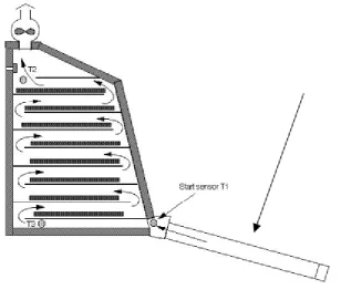
thicknesses ranging between 0.1 m – 0.3 m for air velocities ranging between 1 m/s - 5 m/s. A parametric sweep enables simulation within the specified range of parameter values in one process, without having to do it for discrete values. The purpose of the parametric sweep was to determine the maximum grain layer thickness that would allow the fan to overcome static resistance to airflow.
Once the maximum allowable layer thickness was determined, simulation of air flow up increasing number of grain layers was carried out in order to determine the number of layers the air was able to penetrate. In this case, variation of pressure up the drying cabinet with different grain layer numbers was observed. It was expected that pressure would decrease gradually up the drying cabinet. Any behavior to the contrary would suggest air was not able to penetrate.
43 Figure 3. 1: Model creation
.
Figure 3. 2: Flow chart of preprocessing stage of simulation
Once simulation was complete, post-processing, summarized in Figure 3.3, was carried out to extract the results in various forms as required.
Open SolidWorks
Click Sketch & select plane
Sketch rectangular section & dimension figure
Extrude figure to required dimensions
For chimney, expand fillet, select top, chamfer edges, dimension
Select top face, sketch and extrude circle For plenum, select face,
sketch, extrude rectangle To shell, select inlet & outlet, dimension wall thickness
Open COMSOLMultiphysics &Select Physics (laminar flow)
To import model, select Livelink interfaces
Select Livelink for SolidWorks, Synchronise
Select Defeaturing & repair, Cap faces
Select the materials (wood, air)
44 Figure 3. 3: Post-processing stage of simulation 3.2.2 Sizing of solar dryer
a) Fan power determination
Having found the maximum grain layer thickness to allow penetration by the air to be 0.1 m (section 3.2.1), the simulated pressure drop for this layer thickness was taken as being equivalent to the static pressure to be overcome by the suction fan. This static pressure ( ) as well as the corresponding air flow rate ( ) was applied in
eq. (2.5) to determine the power of the appropriate fan. The results are shown in section 4.1.2.
b) Drying cabinet and solar collector i. Drying cabinet
To determine the cross sectional area of the drying cabinet, a capacity of 18 kg per tray (a mass that an average family would dry for milling, and also that can be carried comfortably when loading) was assumed. The volume (Vgr), of grain per tray
was determined using eq. (3.1), the grain density for maize being 0.76 g/cc. The cross sectional area of the drying cabinet Acb was then determinedfrom eq. (3.2), the
value of (maximum grain layer thickness) having been determined as 0.1 m from
section 3.2.
Select Results, expand Parameter (velocity/pressure), choose slice (1)
To export data, select parameter (velocity/pressure), Export data
For graphs click Results, then ID Plot group, choose type of graph (line)
Choose Define cut line and appropriate section, plot
For report, Choose Result, Report, type of report (complete), form of report (ms word), image (jpeg)