On The Distribution of Linear Biases:
Three Instructive Examples
Mohamed Ahmed Abdelraheem1, Martin ˚Agren2, Peter Beelen1, and Gregor Leander1
1
Technical University of Denmark, DK-2800 Kgs. Lyngby, Denmark
{M.A.Abdelraheem,P.Beelen,G.Leander}@mat.dtu.dk 2
Dept. of Electrical and Information Technology, Lund University, P.O. Box 118, SE-221 00 Lund, Sweden
Abstract. Despite the fact that we evidently have very good block ci-phers at hand today, some fundamental questions on their security are still unsolved. One such fundamental problem is to precisely assess the security of a given block cipher with respect to linear cryptanalysis. In by far most of the cases we have to make (clearly wrong) assumptions, e.g., assume independent round-keys. Besides being unsatisfactory from a scientific perspective, the lack of fundamental understanding might have an impact on the performance of the ciphers we use. As we do not understand the security sufficiently enough, we often tend to embed a se-curity margin – from an efficiency perspective nothing else than wasted performance. The aim of this paper is to stimulate research on these foundations of block ciphers. We do this by presenting three examples of ciphers that behave differently to what is normally assumed. Thus, on the one hand these examples serve as counter examples to common beliefs and on the other hand serve as a guideline for future work.
1
Introduction
IT Security plays an increasingly crucial role in everyday life and business. When talking on a mobile phone, when withdrawing money from an ATM or when buying goods over the internet, security plays a crucial role in both protecting the user and in maintaining public confidence in the system. Moreover, security techniques are often an enabler for innovative business models, e.g., iTunes and the Amazon Kindle require strong copyright protection mechanisms, or after-sale feature activation in modern cars. Virtually all modern security solutions are based on cryptographic primitives. Block ciphers are arguably the most widely used type of these primitives.
Besides being unsatisfactory from a scientific perspective, the lack of funda-mental understanding might have consequence on the performance of the ciphers we use. As we do not understand the security sufficiently, we tend to embed a security margin in the ciphers we are using. From an efficiency perspective, a security margin is nothing else than wasted performance. While for some appli-cations this might not be critical, for others it certainly is. In particular, when it comes to cryptography in the emerging field of pervasive computing, the com-putational resources of the devices in question are often highly constrained, and we can only allow close to zero overhead for a security margin.
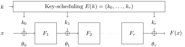
Especially for the key-scheduling algorithm, the fundamental part of a cipher that is responsible for generating key-material from a master-key to be used at several places in the algorithm (see Figure 1 for an example), simplifying assumptions are standard. While these assumptions are strictly speaking wrong, the hope is that the behaviour of the real cipher does not differ significantly from the simplified model.
Linear Cryptanalysis One of the best known and most general applicable attacks on block ciphers is Matsui’s linear attack [17]. Since its introduction many extensions and improvements have been made, and we mention a selection here. A more precise estimate for the success probability and the data complexity are given by Sel¸cuk [22]. The effect of using more than one linear trail, referred to as linear hulls, has been introduced by Nyberg [19]; see also Daemen and Rijmen [9]. This has been used for example by Cho [7]. Multi-dimensional linear attacks have been studied by Hermelin, Cho, and Nyberg [11] as a way to further reduce the data complexity of the basic attack. We also like to mention the critics on the concept of linear hulls by Murphy [18]; see Leander [15] for a further discussion. One of the most recent developments is the idea to make use of unbiased linear approximations by Bogdanov et al. [4].
However, despite its discovery more than 15 years ago, and the many exten-sions introduced since then some very fundamental properties are not yet well understood.
In a nutshell, for claiming a cipher secure against linear attacks, one has to demonstrate that the cipher does not possess certain statistical irregularities. In almost all cases the best we can do is to bound the correlation of a single linear trail, as this roughly corresponds to bounding the number of active Sboxes. Thus, using for example the well established wide-trail strategy used in AES [9], ob-taining strong bounds on the correlation of a single trail is quite easy nowadays. However, when it comes to bounding the correlation of a linear approximation, or linear hull to emphasize its relation to many linear trails, no general con-vincing arguments are available. More precisely, the task of understanding the distribution of linear correlations over the keys is unsolved.
While independent round-keys are hardly ever used in any real cipher, this assumption is on the one hand needed to make the analysis feasible and on the other hand often does not seem problematic as even with the keys not inde-pendently and uniformly chosen, most ciphers (experimentally) do not behave different from the expectation.
However, those experimental confirmations that the cipher behaves as as-sumed are inherently insufficient. For a 128 bit block cipher a single linear ap-proximation that for a fraction of 2−30of all keys has a correlation greater than 2−30 is something that, on the one hand, we clearly want to avoid but, on the other hand, we will never discover by experiments only.
Thus, it is important to really understand the distribution of bias, where the distribution is taken over all possible keys. Only by studying the entire distribu-tion can weak keys possibly be identified (this has been pointed out previously, cf. for example [9]). Promising results along these lines include the work of Dae-men and RijDae-men [10] where the problem is clearly stated and attempts are made to give general statements. Unfortunately, as we will discuss below, one of the most general theorems is strictly speaking wrong.
Our Contribution The aim of this paper is to stimulate research on the foun-dations of block ciphers. We do this by presenting three examples of ciphers that behave differently to what is normally assumed. Thus, on the one hand these ex-amples serve as counter exex-amples to common beliefs and on the other hand serve as a guideline for future work. The value of our examples as guidelines for future work is specific for each example. The first example mainly limits the most gen-eral statements one can hope to prove, and in particular is a counter example to Theorem 22 in [10] where under rather natural conditions it was stated that the distribution of correlations is well approximated by a normal approximation and in particular one should expect many different possible values for the bias. The second example considers the influence of the key scheduling on the distribution of correlations. Here the variance (but not the shape) of the distribution signifi-cantly depends on the key-scheduling. For future work this suggests that highly non-linear key scheduling algorithms are superior to linear ones with respect to the distribution of correlations. Here highly non-linear has to be understood not as a vague criteria but in terms of minimizing the absolute values for all linear approximations. The last example is again related to key-scheduling but more so to symmetries in ciphers. We show a general equivalence of symmetries and linear approximations for weak-keys that exist for any number of rounds and illustrate this fact with an example.
The techniques used to analyze these examples are surprisingly diverse and of independent interest.
2
Notation and Preliminaries
Given an nbit functionF :Fn
2 →Fn2, alinear approximation is an equation of the form
hα, xi+hβ, F(x)i= 0,
whereh·,·idenotes an inner product. The vectorαis called the input mask and
β is the output mask. Thebias F(α, β)∈[−1/2,1/2] of a linear approximation is defined as
Prob(hα, xi+hβ, F(x)i= 0) =1
2 +F(α, β),
where the probability is taken over all inputsx. The bias is the value of major importance for linear attacks. However, due to scaling reasons, it is much more convenient to work with thecorrelationcF(α, β)∈[−1,1] defined by
cF(α, β) = 2F(α, β).
Another measure that we are going to use is the Fourier-transformation ofF,
b
F(α, β) = X x∈Fn2
(−1)hβ,F(x)i+hα,xi.
Up to scaling Fb(α, β) is equivalent to the bias F(α, β) and the correlation
cF(α, β). More precisely,
F(α, β) =
cF(α, β)
2 =
b
F(α, β)
2n+1 . (1)
Linear Trails and Linear Hull Given a composite functionF, i.e.,Fi:Fn2 → Fn2 such thatF=Fr◦· · ·◦F2◦F1, alinear trailθis a collection of all intermediate masks
θ= (θ0=α, . . . , θr=β) and its correlation is defined by
Cθ= Y
i
cFi(θi, θi+1).
It is well known, see e.g., [9], that the correlation of a linear approximation is the sum of all correlations of linear trails starting with the same mask α and ending with the same maskβ, i.e.,
cF(α, β) =
X
θ|θ0=α,θr=β
Cθ. (2)
Key-schedulingE(k) = (k0, . . . , kr) k
x
k0
F1
k1
F2 Fr
kr
F(x)
θ0 θ1 θr
Fig. 1.A key-alternating cipher
in Fig. 1. An nbit key-alternating cipher with ak bit (master) key consists of round functionsFi:Fn2 →Fn2 and a key-scheduling algorithmE:Fk2 →F
n(r+1)
2 .
The dependence of the correlation of a linear trail is conceptually very simple, only the sign of the correlation depends on the key. More precisely,
Cθ= (−1)hθ,E(k)i Y
i
cFi(θi, θi+1).
Plugging this into Equation (2) leads to the following result.
cF(α, β) =
X
θ|θ0=α,θr=β
(−1)hθ,E(k)i+σθ|C
θ| (3)
It is exactly this equation that is often referred to as thelinear hull: The correla-tion of a linear approximacorrela-tion is the key-dependent signed sum of the correlacorrela-tion of all trails.
In this work we are interested in the distribution over the keys of the linear correlation. Here one can think of each linear trailCθas a random variable with a fixed absolute value that with probability 1/2 is positive and with probability 1/2 is negative. In this setting the linear hull is the sum of those random variables. While in general not a lot is known about this distribution, two important characteristics can be stated, assuming independent round-keys. First, as the average of a sum of random variables is the sum of the averages, the average bias is zero. Here, independent round-keys are used to ensure that each single trail has average zero. Moreover, it is easy to see that two distinct linear trails
Cθ and Cθ0 are pairwise independent. It follows (cf. Theorem 7.9.1 in [9]) that with independent round-keys the variance of the distribution, i.e., the average square correlation, is the sum of the squares of the correlations of all trails. We summarize this in the following proposition.
Proposition 1. Assuming independent round-keys, i.e.,k=n(r+1)andE(k) =
k, the average correlation is zero, i.e.,
E(Cθ) = 0.
Moreover, the average square correlation is given by
E(Cθ2) = X
i
Finally, we already note here an observation that we will make use of later. Lemma 1. If the key-scheduling E : Fk2 → F
n(r+1)
2 is linear then two distinct
linear trailsCθ andCθ0 are either independent or Cθ=±c·Cθ0 for a constantc.
More precisely Cθ and Cθ0 are independent if and only if E∗(θ+θ0)6= 0 where
E∗ is the adjoint linear mapping.
Proof. The lemma follows directly from the observation that
hθ, E(k)i+hθ0, E(k)i=hE∗(θ), ki+hE∗(θ0), ki=hE∗(θ+θ0), ki
and the general remark that a linear function`(·) =ha,·i is either balanced (if
a 6= 0) or constant (if a = 0). Thus two trails are independent if and only if
E∗(θ+θ0)6= 0. ut
3
Our Results
In this section we briefly describe our examples, the results and their interpre-tation. As the first and the last example require more technical details for a full explanation, the exact analysis of those results and their proofs are given in later sections.
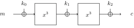
3.1 Example I: The Cube-Cipher
As a first example, we study the two round key-alternating cipher depicted in Fig. 2 with block sizen,nodd. The round functionx→x3has to be understood as a mapping on the finite field F2n with 2n elements (as n is odd this is a bijection). The key consists of three independent subkeys k0, k1, k3 each of n bits. Obviously, and for various reasons [13, Section 8.4], this is an artificial example of a block cipher. However, for the purpose of this counterexample that does not matter – it is a counterexample anyway. Moreover, as this cipher clearly belongs to the class of key-alternating ciphers, general theorems on these have to either explicitly exclude this (and similar) examples or the statements have to cover this strange behavior as well.
m
k0
x3
k1
x3
k2
c
Fig. 2.TheCube-cipher
the same absolute correlation. This seems the ideal situation (we even have a parameter, n, that could go to infinity) for assuming that the distribution of correlations over the keys is very well approximated by a normal distribution, cf. Theorem 22 in [10].
Theorem 1 (Theorem 22 of [10]). Given a key-alternating cipher with in-dependent round-keys. If the number of linear trails with non-zero correlation is large and the square of the correlation of each linear trail is small compared to the variance of the distribution then the distribution is well approximated by a normal distribution.
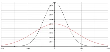
The intuition why a normal distribution should be a good approximation is that in this case the linear hull is the sum of a huge amount of pairwise(!) independent random variables. However, it turns out to be wrong. In particular, for any n, the correlation of the cipher actually takes only 5 different values. Thus, the roughly 2n−2 random variables are not independent at all. As an example of the real distribution compared to the assumed normal distribution we consider the case n = 31 (other cases behave very similarly). Figs. 3(a) and 3(b) show both distributions and make clear that the normal approximation is not a very good approximation and in particular does not get substantially better whenn
increases. In Section 4 we prove that in general only 5 values are obtained and we furthermore study the exact distribution of those 5 values.
(a) The (normalized) distribution of the
Cube-cipher vs the normal distribution
(b) The (normalized) cumulative probabil-ity distribution of the Cube-cipher vs the normal distribution
3.2 Example II: PRESENT with identical round-keys
Our second example is related to the block cipher PRESENT by Bogdanov et al., see [3] for details. As was previously shown, e.g., by Ohkuma [21], for an increasing number of rounds PRESENT exhibits many linear trails with only one active Sbox per round. Due to the design criteria of the Sbox, it follows that all those trails have the same linear bias. Besides, those trails are the ones with a maximal correlation (in absolute terms).
It was experimentally confirmed in [21] that the distribution of the correlation nicely follows a normal-distribution with mean zero and variance 2(−2r−1)2N whereN is the number of the linear trails with only one active Sbox per rounds. Thus, experimentally, we can notice two facts: Firstly, for PRESENT different trails behave like independent random variables (in contrast to theCube-cipher) and secondly, the contribution of the non-optimal trails does not influence the distribution significantly.
Let us now come to a variant ofPRESENT with identical round-keys1 (and round-constants to avoid trivial slide attacks [1]). As it turns out this is an in-triguing example of the influence of the key-scheduling on the distribution of the correlations. We started by performing experiments on a large number of random keys and observed that the total variance of the bias distribution for some linear approximations of PRESENT with identical round-keys is consistently bigger than that of standard PRESENT for any number of rounds ≥5. Fig. 4 shows the distribution of the linear correlation for the identical round-keys case vs. the originalPRESENT key-scheduling for 17 rounds.
Fig. 4. The (normalized) probability distribution of the PRESENT-cipher with the usual vs the identical round-keys case
The difference is significant in the sense that more rounds of PRESENT with identical round-keys are vulnerable to linear attacks for a non-negligible fraction of keys. In other words, in this example it is indeed the choice of the key-scheduling that makes the cipher secure or insecure against linear cryptanalysis.
1
To illustrate the difference consider a 20 round version. The fraction of keys with a squared bias larger than 2−55 is 33.7% in the case of identical round-keys but only 1.1% in the case of the standardPRESENT key-scheduling.
For computing the variance of a sum of random variables it is sufficient to study the pairwise covariance of the summands. Now, as mentioned above in Lemma 1 for a linear key-scheduling algorithm there are only two possibilities for the covariance. Either two trails are independent or identical up to a constant factor. In our particular case this constant is either 1 or −1 as all trails we consider have the same absolute correlation. Note furthermore that, following Lemma 1, two trailsCθandCθ0 are identical (up to a constant±1) iffE
∗(θ+θ0) =
0 whereEdenotes the key-scheduling function. For identical round-keys, we have that E(k) = (k, . . . , k) and thus
E∗(θ) =E∗(θ0, . . . , θr) = r X
i=0
θi.
In other words two trails are identical iff the (xor) sums of all intermediate masks are identical. While in general, computing the number of trails is much more efficient than listing all trails, it is still feasible for r≤20 to compute the list of trails and sort this list according to the sum of the intermediate masks. Thus, for r ≤ 20 we can relatively easily compute the expected variance for the PRESENT-variant with identical round-keys. Table 1 shows the expected variance (Var2) of the bias distribution of the optimal linear approximation for a specific one bit input and output difference. ForPRESENT with identical round-keys the expected variance is very close to the observed variance (ObsVar) sampled over 20000 random keys. Table 1 also shows the expected variance of the bias distribution of the optimal linear approximation of (standard)PRESENT (Var1) along with the number of trails (N1) with one active Sbox per round, and the number of trails (N2) where the sign depends on the keybits, for number of roundsr, 15≤r≤20.
Table 1.Analytical and experimental data onr-round reducedPRESENT(possibly with identical round-keys).N1is the number of all linear trials with one active Sbox.N2
is the number of trails (amongN1) that don’t behave the same (their absolute values
are equal but the correlation sign is different and it changes according to the subkeys). Var1 gives the expected variance of the bias of the optimal linear approximation of
(standard)PRESENT, while Var2 corresponds toPRESENT with identical round-keys. ObsVar is the experimentally observed variance sampled over 20000 random round-keys.
r N1 N2 log2(Var1) log2(Var2) log2(ObsVar)
It is important to note that, while theCube-cipher is certainly an artificial design, PRESENT with identical round-keys is not. In this context we like to mention that it is precisely the behavior described here that resulted in the need to choose a different Sbox in thePRESENT-inspired sponge-based hash-function
SPONGENTby Bogdanov et al. [2].SPONGENTcan be seen as a fixed key
and large block size variant ofPRESENT with identical round-keys.
3.3 Example III: PRINTcipher or Block Ciphers with Symmetries
It was already pointed out by Leander et al. [16] that for PRINTcipher-48 [12] by Knudsen et al. there exist strongly biased linear relations for any number of rounds. More precisely,
Proposition 2 (Corollary 2 in [16]). For a fraction of 2−28 of all keys
and for any round r ≤ 48 there exists at least one linear approximation for
PRINTcipher-48 with correlation at least2−16−2−32.
Here (cf. Section 5), we extend upon this analysis by showing an equivalence between a submatrix Aof the correlation matrix that has an eigenvector with eigenvalue one and a round function that has an invariant subspace. This is cru-cial as this implies that this sub-matrixA, when taken to ther-th power, does not converge to the all-zero matrix. In particular in the case where there is a unique eigenvector with eigenvalue of norm 1,Arconverges to a non-zero constant.This
is equivalent to saying that trails with all intermediate masks determined by the invariant subspace cluster significantly for any number of rounds.
Note that an invariant subspace in particular captures, as a special case, what is usually referred to as symmetries. Thus, besidesPRINTcipherone could also imagine an identical-round-key variant of AES with round constants that do not destroy the symmetries introduced by the very structured and byte oriented linear layer of AES. This example reveals two interesting points. First, in such a situation of trail clustering, increasing the number of rounds does not help and secondly without the link to invariant subspaces it seems very hard to understand why certain trails should cluster even for an AES-like design that follows the wide-trail strategy. Moreover this clustering is not inherently limited to ciphers with weak mixing (e.g., PRINTcipher), but is rather a problem for all ciphers exhibiting symmetries.
Interestingly, in a restricted sense to be discussed in Section 5, the reciprocal statement holds as well. That is, if the cipher does not exhibit symmetries, then no sub-matrices (of a certain type) have eigenvectors (of a certain type) with eigenvalue 1. Thus by avoiding symmetries one also ensures that trail clustering for any number of rounds is highly unlikely.
2−21 Bias
(a) The non-weak xor keys
2−9.0 Bias
(b) The weak xor keys
Fig. 5.The distribution ofPRINTcipher-24 biases for a fixed permutation key. The experimentally observed meansm are indicated. In both distributions, the standard deviationσis approximately 2−13.0. Ticks have been placed atm+kσ,k∈ {−3, . . . ,3}.
4
Example I: The
Cube
-Cipher
In this section we give a detailed analysis of the distribution of the correlations in theCube-cipher2.
We denote the block size byn, where in this examplenhas to be odd. First note that the initial and the final key-addition do not change the distribution. Thus, to simplify notation, we ignore them from now on. We therefore have to consider the functionFk(x) = (x3+k)3. Moreover, to make the analysis easier, we focus on the input and output mask 1∈ F2n. That is, we are interested in the distribution ofFbk(1,1) for varying key k.
As a first step we show that the corresponding linear hull contains a very large number of trails with non-zero correlations. More precisely, the following holds (cf. Appendix A for the proof).
Theorem 2. The number t of trails with non-zero correlation of the form
1 x
3
→αx
3
→1
is
t= 2
n+ 1−(an
1 +an2+an3+an4)
4 ,
where ai are the four (complex) roots of the polynomial x4+x3+ 2x+ 4.
Fur-thermore, each trail has a correlation of ±21−n.
The next proposition shows that, despite the huge number of non-zero trails, only 5 values occur for the correlations.
Proposition 3. Fbk(1,1)∈ {0,±2 n+1
2 ,±2
n+3 2 }
2
Proof. We denote byµ(x) = (−1)Tr(x), where Tr(x) =x+x2+x4+. . . x2n−1
is the trace mapping and note that Tr(xy) is the natural inner product onF2n.
b
Fk(1,1)2= X
x,y
µ (x3+k)3+ (y3+k)3+x+y
=X
x,y
µ ((x+y)3+k)3+ (y3+k)3+x
=X
x
µ (x3+k)3+x+k3 X y
µ x64+ (k16+k4)x16+ (k8+k2)x4+x
y8
= 2n X x∈M
µ (x3+k)3+x+k3
where
M ={x|x64+ (k16+k4)x16+ (k8+k2)x4+x= 0}.
Thus, we have to understand the kernel (and in particular its size) of the F2 -linear mapping
P(x) =x64+ (k16+k4)x16+ (k8+k2)x4+x.
As a polynomial,P splits nicely into factors, i.e.,
P(x) =A1(x3)A2(x3)A3(x3)A4(x3)x, with
A1(x) =x3+k2x+ 1 A3(x) =x6+x4+ (k4+k2+ 1)x2+x+ 1
A2(x) =x3+ (k2+ 1)x+ 1 A4(x) =x9+x3+ (k8+k2)x+ 1.
For now, we show thatA3(x) does not have any roots. Note that this is actually enough to prove the proposition, as this upper bounds the number of elements inM by 16 = 9 + 3 + 3 + 1 and for general reasons we know that|M|= 2i with
iodd. Thus |M| ∈ {2,8}. Assume thatA3(x) = 0. Then
k4+k2+ 1 = x
6+x4+x+ 1
x2 =x
4+x2+1
x+
1
x2.
Applying the trace mapping to both sides implies Tr(1) = 0.3 A contradiction,
asnis odd. ut
This already demonstrates an unexpected behavior. The following theorem, proven in Appendix B, allows us to compute the exact distribution of the 5 occurring values for reasonably large n.
Theorem 3. We have
#{k∈F2n|Fbk(1,1)2= 2n+3}= 1
3#{β ∈F2n|β satisfies Eqns. (4)}, 3
where
Tr
1 (β2+β)
1/9!
= 1 Tr
β3 β2+β
1/9!
= 1 Tr
(1 +β)3
β2+β 1/9!
= 1(4).
The advantage of the above theorem is that it gives a fast way to compute the numberAofk∈F2n such thatFbk(1,1) = 2n+3. Let us further denote byB the number ofk∈F2n such thatFbk(1,1) = 2n+1. Then clearly
X
k b
Fk(1,1)2=A2n+3+B2n+1.
On the other hand, since knowing the number of trails with non-zero correlation together with their correlation values, corresponds to knowing the average square correlation, we have
X
k b
Fk(1,1)2= 2−n X
α b
C(1, α)2Cb(α,1)2.
Using the above and Theorem 2 we see that
A2n+3+B2n+1=X k
b
Fk(1,1)2= 2n(2n+ 1−a1n−an2−an3−an4),
where, as in Theorem 2,ai are the four (complex) roots of the polynomialx4+
x3+2x+4. Thus using Proposition 3 and the symmetry of the distribution (which can easily be proven in this case) one can now obtain the complete distribution for how manyk,Fk(1,1) obtains a particular value in {±2(n+3)/2,±2(n+1)/2,0} for reasonably large values of n. We give some examples below.
n −2(n+3)/2 −2(n+1)/2 0 2(n+1)/2 2(n+3)/2
1 0 1 0 1 0
3 1 0 6 0 1
5 0 6 20 6 0
9 10 90 312 90 10
19 10868 87078 328396 87078 10868
31 44732008 357939982 1342139668 357939982 44732008
5
Example III:
PRINTcipheror Block Ciphers with
Symmetries
The results in this section, especially as summarized in Theorem 5, are quite general, applying to any block cipher (permutation) exhibiting these kinds of symmetries. For this reason, we do not describe PRINTcipher in detail here, but refer to Appendix D or [12] instead. We only note here that the round-key is the same in every round (there is a small round constant).
The Invariant Subspace Let us define a subspace U ⊂ Fn
2, the orthogonal subspace U⊥ = {y : hx, yi = 0,∀x ∈ U⊥} and a constant d ∈ Fn
2. Then, the invariant subspace property (cf. [16]) can be expressed asFi(U+d) =U+d. In the case of PRINTcipher, the exact definitions of U, U⊥, and d can be found in Appendix E. We only note that for PRINTcipher, |U +d| = 216, and the trails do not involve the round constants so the invariant subspace extends to the entire cipher F, regardless of the number of rounds. However, even if an invariant subspace only occurs for some rounds of the cipher, it can certainly be interesting in linear cryptanalysis as seen below.
Understanding the Large Correlations The correlation matrix (cf. [9])
Mi = (cFi(α, β))αβ collects all correlation coefficients for a single round. We are interested in the submatrix A = (aαβ)α,β∈U⊥ constructed through aαβ =
cFi(α, β) and its powers A
r. ThusA collects the correlations where input and output masks only involve the bits that govern the invariant subspace. In any correlation matrix, the first row and column are all-zero except forc(0,0) = 1. We extract the sub-matrixB = (aαβ)α,β∈U⊥\{0}, since it will be slightly more
convenient to use.
We should identifyAi withFi, but the round constants do not affectAi, so allAi are equal. In particular ArAr−1. . . A1 =Ar. Note howAr describes the contribution to the linear hull from following trails with intermediate masks in
U⊥. More specifically, we can write Equation (3) as
cF(α, β) =
X
θ |θ0 =α,θr=β, θi∈U⊥,∀i
(−1)hθ,E(k)i+σθ|C θ|+
X
θ| θ0 =α,θr=β,
∃i:θi /∈U⊥
(−1)hθ,E(k)i+σθ|C θ|,
where the first sum corresponds to element (α, β) ofAr. If elements ofArhave a large magnitude, then the corresponding elements ofMrhave (at least) the same magnitude, unless the contributions from trails that go outsideU⊥ (essentially) cancel those from inside.
We now examine the asymptotic behaviour ofAr. Define v = (v
α)α∈U⊥ by
vα= (−1)hd,αi.
Lemma 2. vT is an eigenvector to Awith eigenvalue 1, i.e., AvT =vT. We prove this lemma in Appendix C.1.
Now, in the case where there is no other (non-trivial) eigenvector with eigen-value 1 the sequenceAr will converge (see the theorem below). This motivates the following definition.
Definition 1. If the algebraic multiplicity ofA’s eigenvalue1is two andA has no other eigenvalue of absolute value 1, we say that A (or the corresponding cipher) has a stable symmetry. (The eigenvectors are that given in Lemma 2, and the vector(1,0,0, . . . ,0)T.)
For the following theorem, we use thatAhas eigenvalues with absolute value at most 1, the Schur decomposition ofA and the relation between convergence of
Theorem 4. IfAhas a stable symmetry thenBr→C= 1 2dim(U)−1u
Tu,r→ ∞,
u= (vα)α∈U⊥\{0}.
If other contributions tocF(α, β) are negligible, then all characteristics with non-zeroα, β∈U⊥havecF(α, β)≈ ±2−dim(U)so biasF(α, β)≈ ±2−dim(U)−1.
Equivalence Between Eigenvectors and Invariant Subspaces With the following theorem, which we prove in Appendix C.2, we establish a loose relation between symmetries in block ciphers and susceptibility to linear cryptanalysis. In the case of PRINTcipher, this was a negative result, but in case of block ciphers without symmetries, it is positive.
Theorem 5. Consider an invertible vectorial Boolean function F, a subspace
U, the orthogonal subspace U⊥ and a vector d. Define A = (aαβ)α,β∈U⊥ and
v= (vα)α∈U⊥,vα= (−1)hd,αi. ThenAvT =vT if and only ifF(U+d) =U+d.
Experimental Results onPRINTcipher We have implementedPRINTcipher -48 for a key from the class of weak keys used as the main example in [16]. This allowed us to derive A and verify that AvT = vT. We could also derive the biases for 16 characteristics with α, β ∈ U⊥. All of them were close to ±2−17 as suggested by the above analysis. This gives some circumstancial support to the idea thatB48≈C, that this is the main contribution toc
F(α, β), and that PRINTcipheractually has a stable symmetry.
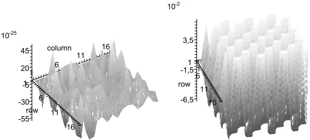
OnPRINTcipher-12, we can deriveB12 analogously to above. Here the sta-ble symmetry can then be confirmed by deriving the eigenvalues numerically for all possible matricesB12. Also, the convergence can be observed experimentally. Fig. 6(a) showsB100
12 for a non-weak key, while Fig. 6(b) corresponds to a weak key. The matrices clearly differ both in terms of magnitude and structure. Fur-thermore convergence is rather fast, B10
12 is already very close to the expected limit.
6
Conclusion and Future Work
We presented and analyzed three interesting examples of ciphers with a non-expected distribution of correlations. The first example mainly limits the most general statements one can hope to prove. General theorems on key-alternating ciphers have to deal with this strange behavior as well.
The second example considered the influence of the key scheduling on the distribution of correlations. For future work this suggests that highly non-linear key scheduling algorithms might be preferable (cf. also [20]). To see this con-sider the covariance between two different non-zero trails Cθ and Cθ0 for θ =
(a) The matrixB12100for a non-weak key (b) The matrixB 100
12 for a weak key
Fig. 6.The matrixB10012 for two different keys
δ = (θ2+θ02, . . . , θr−1+θ0r−1) andE0(k) = (E2(k), . . . , Er−1(k)), in this setup the covariance is essentially determined by
X
k
(−1)hθ+θ0,E(k)i=X k
(−1)hδ,E0(k)i+hγ,ki,
which is nothing else than the Fourier coefficientEc0(γ, δ). Thus minimizing all covariances corresponds to minimizing the absolute value of Ec0(γ, δ) which in turn corresponds exactly to maximizing the nonlinearity ofE0.
The last example is again related to key-scheduling but more so to symme-tries in ciphers. We show a general equivalence of symmesymme-tries and linear approx-imations for weak keys that exist for any number of rounds. This is actually a positive result as it suggests that avoiding these symmetries makes clustering of trails unlikely. Future work is needed to either make this equivalence tighter or find examples of round-independent trail clustering that does not originate from symmetries.
We hope that this work stimulates further research on this fundamental topic.
Acknowledgments The second author was supported by the Swedish Foun-dation for Strategic Research (SSF) through its Strategic Center for High Speed Wireless Communication at Lund.
References
2. A. Bogdanov, M. Knezevic, G. Leander, D. Toz, K. Varici, and I. Verbauwhede. SPONGENT: A lightweight hash function. In B. Preneel and T. Takagi, edi-tors, CHES, volume 6917 of Lecture Notes in Computer Science, pages 312–325. Springer, 2011.
3. A. Bogdanov, L. R. Knudsen, G. Leander, C. Paar, A. Poschmann, M. J. B. Rob-shaw, Y. Seurin, and C. Vikkelsoe. PRESENT: An ultra-lightweight block cipher. In P. Paillier and I. Verbauwhede, editors,CHES, volume 4727 ofLecture Notes in Computer Science, pages 450–466. Springer, 2007.
4. A. Bogdanov and M. Wang. Zero correlation linear cryptanalysis with reduced data complexity. InFSE, 2012.
5. M. L. Buchanan and B. N. Parlett. The uniform convergence of matrix powers.
Numerische Mathematik, 9(1):51–54, 1966.
6. C. Carlet. Boolean functions for cryptography and error-correcting codes. In Y. Crama and P. L. Hammer, editors,Boolean Models and Methods in Mathemat-ics, Computer Science, and Engineering, pages 257–397. Cambridge University Press, 2010.
7. J. Y. Cho. Linear cryptanalysis of reduced-round PRESENT. In J. Pieprzyk, editor, CT-RSA, volume 5985 of Lecture Notes in Computer Science, pages 302– 317. Springer, 2010.
8. J. Daemen, M. Peeters, G. V. Assche, and V. Rijmen. Nessie proposal: NOEKEON. http://gro.noekeon.org/Noekeon-spec.pdf, 2000.
9. J. Daemen and V. Rijmen.The design of Rijndael: AES - the Advanced Encryption Standard. Springer, 2002.
10. J. Daemen and V. Rijmen. Probability distributions of correlation and differentials in block ciphers. IACR Cryptology ePrint Archive, 2005:212, 2005.
11. M. Hermelin, J. Y. Cho, and K. Nyberg. Multidimensional extension of Matsui’s algorithm 2. In O. Dunkelman, editor, FSE, volume 5665 of Lecture Notes in Computer Science, pages 209–227. Springer, 2009.
12. L. R. Knudsen, G. Leander, A. Poschmann, and M. J. B. Robshaw.PRINTcipher: A block cipher for IC-printing. In S. Mangard and F.-X. Standaert, editors,CHES, volume 6225 ofLecture Notes in Computer Science, pages 16–32. Springer, 2010. 13. L. R. Knudsen and M. Robshaw. The Block Cipher Companion. Information
security and cryptography. Springer, 2011.
14. Gilles Lachaud and Jacques Wolfmann. The weights of the orthogonals of the ex-tended quadratic binary goppa codes. IEEE Transactions on Information Theory, 36(3):686–692, 1990.
15. G. Leander. On linear hulls, statistical saturation attacks, PRESENT and a crypt-analysis of PUFFIN. In K. G. Paterson, editor, EUROCRYPT, volume 6632 of
Lecture Notes in Computer Science, pages 303–322. Springer, 2011.
16. G. Leander, M. A. Abdelraheem, H. AlKhzaimi, and E. Zenner. A cryptanalysis of
PRINTcipher: The invariant subspace attack. In P. Rogaway, editor,CRYPTO, volume 6841 ofLecture Notes in Computer Science, pages 206–221. Springer, 2011. 17. M. Matsui. Linear cryptanalysis method for DES cipher. In T. Helleseth, editor,
EUROCRYPT, volume 765 ofLecture Notes in Computer Science, pages 386–397. Springer, 1993.
18. S. Murphy. The effectiveness of the linear hull effect.Technical report, RHUL-MA-2009-19, 2009.
20. K. Nyberg. Comments on key-scheduling, 2012. Personal communication. 21. K. Ohkuma. Weak keys of reduced-round PRESENT for linear cryptanalysis. In
M. J. Jacobson Jr., V. Rijmen, and R. Safavi-Naini, editors, Selected Areas in Cryptography, volume 5867 ofLecture Notes in Computer Science, pages 249–265. Springer, 2009.
22. A. A. Sel¸cuk. On probability of success in linear and differential cryptanalysis. J. Cryptology, 21(1):131–147, 2008.
A
Proof of Theorem 2
In this section we prove the following theorem.
Theorem 6. The number t of trails with non-zero correlation of the form
1 x
3
→αx
3
→1
is
t=2
n+ 1−(an
1 +an2+an3+an4) 4
where ai are the four (complex) roots of the polynomial x4+x3+ 2x+ 4.
Fur-thermore, each trail has a correlation of ±21−n.
For the ease of notation, we define
C:F2n→F2n
C(x) = x3.
A trail
1→α→1
has a non-zero correlation if and only if
b
C(1, α)6= 0 and Cb(α,1)6= 0
We make use of the following known lemma.
Lemma 3.
b
C(α, β)2=
0 if Tr(αβ−1/3) = 0and(α, β)6= (0,0) 22n if(α, β) = (0,0)
Proof.
b
C(α, β)2=X x,y
µ(βx3+αx+βy3+αy)
=X
x,y
µ(β(x+y)3+α(x+y) +βy3+αy)
=X
x
µ(βx3+αx)X y
µ(βx2y+βxy2)
=X
x
µ(βx3+αx)X y
µ(y2(β2x4+βx))
= 2n X
x|β2x4+βx=0
µ(βx3+αx)
Note that the equation
β2x4+βx= 0
for any non-zero β has exactly two solutions, namely x = 0 and x = β−1/3. Thus, we continue
b
C(α, β)2= 2n1 +µ(ββ−1+αβ−1/3) = 2n1 +µ(1 +αβ−1/3) = 2n1−µ(αβ−1/3)
which proves the lemma. ut
Thus the number of trails 1→α→1 with non-zero correlation is equal to the number of elements in the set
M ={α| Tr(α−1/3) = 1 and Tr(α) = 1} Note that
|M|= X α| Tr(α)=1
1−µ(α−1/3)
2 = 2
n−2−1 2
X
α| Tr(α)=1
µ(α−1/3)
and
X
α| Tr(α)=1
µ(α−1/3) + X α| Tr(α)=0
µ(α−1/3) = 0.
Therefore,
|M|= 2n−2−1 4
X
α| Tr(α)=1
µ(α−1/3)− X α| Tr(α)=0
µ(α−1/3)
= 2n−2+1 4
X
α
Thus, in order to compute |M|it is sufficient to study
X
α
µ(α−1/3+α) =X α
µ(α3+α−1)
This turns out, just as demonstrated in [14] for the inverse function, to be related to a curve. Namely, we have
Tr(α3+α−1) = 0 iff ∃y∈F2n such thatα3+α−1=y+y2
The equation relating α and y gives rise to an projective algebraic curve C defined overF2of genus 2. The number of points Nn onC defined overF2n can be expressed as
Nn= X
α
1 +µ(α3+α−1)= 2n+X α
µ(α3+α−1),
which implies that
|M|= 1 4Nn.
Using the theory of algebraic curves over finite fields, one can obtain a closed formula forNn in terms of the eigenvalues of the Frobenius operator. Since the curve C has genus 2, these can be computed fromN1 andN2. It is easy to see that N1=N2= 4, which gives rise to the formula
Nn = 2n+ 1−(an1+a n 2+a
n 3 +a
n 4),
wherea1, a2, a3, anda4are the complex roots of the polynomialx4+x3+ 2x+ 4. The theorem now follows.
B
Proof of Theorem 3
Before we give the proof of Theorem 3 we state and prove some intermediate results.
Proposition 4. Let α∈ F2n be a root of A1(x). Then Tr(k3) = 1 + Tr(α−3).
Moreover,A1(x)has exactly one root inF2n if and only ifTr(k3) = 0. Similarly
A2(x) has exactly one rootα∈F2n if and only ifTr(k3) = 1. In both cases this
root satisfies Tr(α−3) = 1.
Proof. We only prove the statement forA1(x) (the statement for A2(x) can be shown by replacingkbyk+ 1 in the proof below). Ifαis a root of A1(x), then
k6= (k2)3= (α2+α−1)3=α6+α3+ 1 +α−3.
Taking traces and using that n is odd, we obtain that Tr(k3) = 1 + Tr(α−3). This implies the first part of the proposition and also the last statement, namely that Tr(α−3) = 1 for a root ofA
Now suppose thatα is the only root of A1(x). Then the polynomial A1(x) factors into irreducible parts as follows
A1(x) = (x+α) x2+αx+ (k+α)2 The polynomial
x2+αx+ (k+α)2 is irreducible if and only if the polynomial
x2+x+
(k+α)
α
2
is irreducible. However this implies that
Tr
(k+α)
α
= 1
which is equivalent to Tr(k2/α2) = 0. As k2 = α2+α−1 we conclude Tr(1 +
α−3) = 0, which by the first part of the proposition implies that Tr(k3) = 0. Conversely assume that Tr(k3) = 0. Let Fbe the smallest extension of F2n containing all roots ofA1(x). ThenFcontains an elementαsatisfyingα3+k2α+ 1 = 0 and (by considering the given factorisation ofA1(x) as above) an element
β satisfyingβ2+αβ+ (k+α)2= 0. The extension degree [F:F2n] can be one (in case all roots of A1(x) are in F2n), two (in case exactly one root of A1(x) is in F2n ) or three (in case A1(x) has no roots in F2n). A direct computation shows that the element γ := β/α+α3+k3 ∈
F is a root of the polynomial
x2+x+k3+ 1. However, since Tr(k3) = 0, this polynomial is irreducible. We see that
[F:F2n] = [F:F2n(γ)][F2n(γ) :F2n] = [F:F2n(γ)]2,
which implies that [F:F2n] = 2. Therefore the polynomial A1(x) has exactly 1
root in F2n. ut
One can say more about the dependence of the roots of the polynomials
A1(x), A2(x) and A4(x). In particular we show in the following lemma that a root ofA4(x) gives rise to roots of A1(x) andA2(x). More precisely, we have Lemma 4. Letξbe a root of the polynomialA4(x). Thenξ(ξ+k)6, respectively
ξ(ξ+k+ 1)6, is a root ofA1(x), respectivelyA2(x).
Proof. The lemma follows by a direct computation.
We are now in the situation to give a characterization of the situation when |M|= 8.
Proposition 5. The polynomialsA1(x),A2(x)andA4(x)together have7roots
in F2n if and only if the polynomial A4(x)has exactly three roots. Moreover in
this situation, if Tr(k3) = 0 (resp. Tr(k3) = 1), the polynomial A
2(x) (resp.
Proof. First of al note that Proposition 4 implies thatA1(x) andA2(x) together can have 1 or 4 roots inF2n. Now assume thatA1(x),A2(x) andA4(x) together have 7 roots. ThenA4(x) will have at least one root. The previous lemma then implies thatA1(x) andA2(x) together have at least two roots. Combining, we see thatA4(x) has exactly three roots. Conversely, assumingA4(x) has exactly three roots, one obtains by a similar reasoning that A1(x) andA2(x) together have four roots. The final part of the lemma follows from Proposition 4.
The next goal is to determine for how many k ∈ F2n it happens that b
Fk(1,1)2 = 2n+3. It is not difficult to see that half such k satisfy Tr(k3) = 0, while the other half satisfies Tr(k3) = 1. From now on we will assume that Tr(k3) = 1 and count how manyk∈
F2n satisfyFbk(1,1)2= 2n+3.
Theorem 7. Given k∈F2n such thatTr(k3) = 1 andFbk(1,1)2 = 2n+3. Then
there existsβ ∈F2n such that
(β2+β+ 1)3 (β2+β)2 =k
6 (5)
Tr
1
(β2+β) 1/9!
= 1 (6)
Tr
β3
β2+β 1/9!
= 1 (7)
Tr
(1 +β)3
β2+β 1/9!
= 1. (8)
Conversely, givenβ∈F2nsatisfying Eqns. (6,7,8), there existsk∈F2nsatisfying
Equation (5), Tr(k3) = 1, andFbk(1,1)2= 2n+3.
Proof. First assume thatFbk(1,1)2= 2n+3. We have seen before that a necessary condition is that |M| = 8, which implied that eitherA1(x) or A2(x) has three roots inF2n. Since Tr(k3) = 1 we see using Proposition 4 thatA1(x) has three roots. This is exactly the case ifα, β∈F2n exist such that
k2=α2+α−1and α−3=β2+β.
The three roots ofA1(x) areα(obviously) andαβ andα(β+ 1). This implies
k6= (α2+α−1)3 =α6+α3+ 1 +α−3
= (β2+β)−2+ (β2+β)−1+ 1 +β2+β
= (β
2+β+ 1)3 (β2+β)2 ,
used to defineM. It is easy to see that all other elements of M are just linear combination ofx1,x2, andx3, i.e.
M ={ax1+bx2+cx3 a, b, c∈F2}. In particular
b
Fk(1,1)2=
2n+3if Tr (x3i +k)3+xi
= Tr(k3) = 1∀i
0 else
Thus, we have to compute
Tr (x3i +k)3+xi
.
AsA1(x3i) = 0 it holds that
x9i +k2x3i + 1 = 0,
therefore
Tr (x3i +k)3+xi
= Tr x9i +kx6i +k2x3i +xi+k3
= Tr kx6i +xi+k3+ 1
= Tr k2x1i2 +xi+k3+ 1
.
Usingk2=x6i +x−i3 we get Tr (x3i +k)3+xi
= Tr x18i +x9i +xi+k3+ 1
= Tr xi+k3+ 1
= Tr (xi),
as Tr(k3) = 1. Thus
b
Fk(1,1)2=
2n+3if Tr (x
i) = 1∀i
0 else
The conditions Tr (xi) = 1 are, when expressed in terms ofβ, exactly Equations (6,7,8).
Conversely assume that we are given β ∈F2n satisfying Equations (6,7,8). Since β ∈F2n, there is exactly one k∈F2n satisfying Equation (5). For this k we have
Tr(k3) = Tr(k6) = Tr
(β2+β+ 1)3 (β2+β)2
= Tr
β2+β+ 1 + 1
β2+β + 1 (β2+β)2
Also for this k, the polynomial A1(x) = x3+k2x+ 1 has three roots in F2n, namely (β2+β)−1/3,β(β2+β)−1/3, and (β+1)(β2+β)−1/3.Reasoning as above, we obtain using Equations (6,7,8) thatFbk(1,1)2= 2n+3as desired.
The above theorem gives an alternative way to determine for how many
k∈F2n it happens thatFbk(1,1)2= 2n+3. More precisely, we find Theorem 8. We have
#{k∈F2n|Fbk(1,1)2= 2n+3}= 1
3#{β∈F2n|β satisfies Eqns. (6,7,8)}.
Proof. For convenience we define
S:={β∈F2n|β satisfies Eqns. (6,7,8)}.
As noted before, half of allk∈F2nsatisfyingFbk(1,1)2= 2n+3satisfy Tr(k3) = 0, while the other half satiesfies Tr(k3) = 1. Therefore, the corollary follows once we show that
#{k∈F2n|Fbk(1,1)2= 2n+3,Tr(k3) = 1}= 1
6#S. (9)
We have already seen that there is a correspondence betweenβ∈F2nsatisfying Eqns. (6,7,8) and k ∈ F2n such that Fbk(1,1)2 = 2n+3and Tr(k3) = 1. This correspondence is expressed by Equation (5). Given β ∈ S, there is only one
k ∈ F2n satisfying Equation (5), but the converse is not true. More precisely, givenk, there are six possible solutions to Equation (5). Once one solutions has been fixed, sayβ, the other possibilities can be expressed in thisβ asβ+ 1, 1/β, (β+ 1)β, 1/(β+ 1), and β/(β+ 1). Forβ ∈ F2n\F2, this gives exactly all six distinct solutions to Equation (5). Note that 0 and 1 are not elements ofS. This shows that there is a six to one correspondence between possible values ofβ and
k, thus establishing Equation (9).
C
Proofs of Symmetry-Related Results
C.1 Proving Lemma 2
Proof (Lemma 2).
2n(A·vT)α= 2n X
β∈U⊥
aαβvβ= 2n X
β∈U⊥
2−nFb(α, β)vβ
= X
β∈U⊥
X
x
(−1)hβ,F(x)i+hα,xi+hd,βi
=X
x
(−1)hα,xi X β∈U⊥
A general result states that
X
y∈U⊥
(−1)ha,yi=
|U⊥| ifa∈U,
0 else.
Applying this to the above and using the invariant subspace property, we get
2n(A·vT)α
=|U⊥| X F(x)∈U+d
(−1)hα,xi
=|U⊥|X x∈U
(−1)hα,x+di
=|U⊥|(−1)hα,diX x∈U
(−1)hα,xi,
and as x∈U andα∈U⊥ it holds thathα, xi= 0. So we finally get
2n(A·vT)α=|U⊥||U|(−1)hα,di= 2nvα,
i.e.,vT is an eigenvector ofA, with eigenvalue 1. ut
In Appendix F we give a much more detailed proof, specific toPRINTcipher, where we look at how the individual bits behave: we look at how the linear approximation table of the Sbox is affected by the xor and permutation keys, and how it comes that everything adds up.
C.2 Proving Theorem 5
The “if” part follows from a straightforward generalization of Lemma 2, so we focus entirely on showing the “only if” part. For this, we need the inverse trans-form,
(−1)hβ,F(x)i= 2−nX α
(−1)hα,xi
b
F(α, β).
We first state a general lemma.
Lemma 5. Consider a functionF:Fn2 →F2 and its Fourier transform Fb. Let
U⊥ be a subspace of Fn
2. If2−n P
α∈U⊥(−1)hi,xiFbα= (−1)b, then F(x) =b. In a sense, what this lemma says is that if the calculation ofF(x) from{Fbα}α∈Fn2
appears to be possible using only some subset of Fourier coefficients{Fbα}α∈U⊥,
Proof (Theorem 5).Let us considerβ∈U⊥,x∈U+d. We will study the inverse
F−1 of F. Its Fourier coefficients are d
F−1(α, β) = b
F(β, α). We sum only over
α∈U⊥:
2−n X α∈U⊥
(−1)hα,xi
d
F−1(α, β) = X α∈U⊥
(−1)hα,dia
βα
= X
α∈U⊥
vαaβα=aβ·vT
= 1·vβ= (−1)hd,βi,
whereaβ= (aβα) is a row ofA. By Lemma 5, we can conclude thathβ, F−1(x)i= hβ, di, β ∈U⊥. Since this holds for allβ ∈U⊥, F−1(x)∈(U+d). This holds for all x∈(U+d), soF−1 has the invariant subspace property. Then so does
F. ut
D
PRINTcipherPRINTcipher (of e.g., 48 bits) is constructed as an SPN network that uses a permutation key of 32 bits and an xor key of 48 bits (so in total 80 bits of key). One round of PRINTcipher-48 is shown in Fig. 7, where only a part of the linear layer is shown — the rest has no relevance for the property exploited in [16] or this paper. The lower part of the permutation, after the xor with a round constant, is dependent on the permutation key. Thus, what is shown here corresponds to a particular weak permutation key.
xor sk1
xorRCi
S S S S S S S S S S S S S S S S
E
The invariant subspace
The relevant definitions ofU,U⊥, anddfor the class of weakPRINTcipherkeys used as the main example in [16] are
U ={00* *00 *** *** 00* *00 *** *** 00* *00 *** *** 00* *00 *** ***}, U⊥={**0 0** 000 000 **0 0** 000 000 **0 0** 000 000 **0 0** 000 000},
d=000 010 000 000 000 010 000 000 000 010 000 000 000 010 000 000.
F
A Technical,
PRINTcipher-Specific Proof of Lemma 2
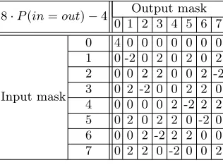
Table 2.Linear Approximation Table (LAT) for the Sbox inPRINTcipher. All non-trivial non-zero values have the same magnitude.
8·P(in=out)−4 Output mask 0 1 2 3 4 5 6 7
Input mask
0 4 0 0 0 0 0 0 0 1 0 -2 0 2 0 2 0 2 2 0 0 2 2 0 0 2 -2 3 0 2 -2 0 0 2 2 0 4 0 0 0 0 2 -2 2 2 5 0 2 0 2 2 0 -2 0 6 0 0 2 -2 2 2 0 0 7 0 2 2 0 -2 0 0 2
We considerPRINTcipherwith a weak key and want to show the eigenvector property,AvT =vT. If one only wants to understand why this property arises in the general case, the proof given in Section 5 is sufficient and simpler. However, in this section, we will take a careful look at what happens insidePRINTcipher, how the individual bits interact with each other and how everything adds up. We attempt to present things from the bottom up, first looking at individual bits and Sboxes, and then gradually moving to larger structures until we reach the entire matrixA.
Table 2 gives the linear approximation table of thePRINTcipherSbox. As all interesting non-zero elements are the same in absolute terms, we will from now on give elements simply as “+” or “-”. This can be done without loss of stringency when they have the same (known) absolute value and it is known how many these non-zero elements are.
in B = Bodd ∪ Beven partitioned into Bodd = {47,43,35,31,23,19,11,7} and Beven={46,42,34,30,22,18,10,6}.
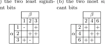
We note that we care about precisely two input and output bits for each Sbox, where the bits indexed in Bodd (Beven) enter the Sboxes inSodd (Seven). Looking at the restrictions of the LAT that arise, there are only two unique such “sub-LATs”. They are given in Tables 3(a) and 3(b). AnactiveSbox is an Sbox with a non-zero input mask. For any input mask, the Sboxes that contribute to the biased output masks are precisely the active Sboxes. The following can be readily verified:
Lemma 6. When the xor key is the all zero key, the Sboxes in Seven use the partial LAT in Table 3(a), while the Sboxes in Sodd use the partial LAT in Table 3(b).
Table 3. Linear Approximation Tables (LATs) for the Sbox in PRINTcipher, re-stricting ourselves to . . .
(a) the two least signifi-cant bits
β
1 2 3
α
1 - +
2 + +
3 +
-(b) the two most signifi-cant bits
β
2 4 6
α
2 + +
4 + +
6 + +
Throughout this section, α ∈ U⊥ is implicitly assumed and r denotes the corresponding row of A, i.e., r = (aαβ)β∈U⊥. (We should write e.g., rα, but
prefer some sloppiness over notation overload.)αis determined by the 16 bitsαn,
n∈ B(α= 247α
47+. . .+ 24α4). We havevα= (−1)hd,αi= (−1)α43+α31+α19+α7. Lemma 7. P
β|rβ| = 1. More precisely, there are 2k non-zero elements of r,
each being±2−k, wherek is the number of active Sboxes with the input maskα.
Proof. It can be seen from Tables 3(a) and 3(b) that each non-zero input mask yields precisely two different output masks. Due to this, there will arise precisely 2k output masks with non-zeror
β. As all non-zero values of the LATs have the same magnitude 2−1, each non-zeror
β will be±2−k. ut
Let us now take the xor key into account. This will change the signs in the LATs. More explicitly, we will now be using three different LATs. They are given in Tables 4(a), 4(b), and 4(c). It is straightforward to derive the following: Lemma 8. With a weak xor key, the Sboxes in Seven use the partial LAT in Table 4(a). The Sboxes inSouter
odd use the partial LAT in Table 4(b), while those
inSinner
Table 4. Linear Approximation Tables (LATs) for the Sbox in PRINTcipher, re-stricting ourselves to some particular choices of xor key bits and . . .
(a) the two least signifi-cant bits
β
1 2 3
α
1 + -2 3 +
-(b) the two most signifi-cant bits
β
2 4 6
α
2 -
-4 + +
6
-(c) the two most signifi-cant bits
β
2 4 6
α
2 + +
4 6
-Proving Lemma 2 amounts to proving thathr, vi=vα, ∀α. Recall that the scalar product is hr, vi = P
β∈U⊥rβvβ. We know from Lemma 7 that r sums absolutely to 1. Sincevα∈ {−1,1}, calculatinghr, viboils down to summing the non-zero elements ofrwith or without a change of sign. Thus, to prove Lemma 2, we need to show that hr, vi ∈ {−1,1}, i.e., the elements ofr are always added constructively, and that the sum isvα (as opposed to−vα).
Lemma 9. Let αn = 0,n /∈ {34,18}. That is, S2 is the only active Sbox with
inputα2 = (α
18, α34)∈ {01,10,11}. Thenhr, vi= +1, so the absolute value of
the scalar product is 1. Further,hr, vi=vα.
Proof. We know from Lemma 7 that there are two nonzerorβ’s. First note that
vβ = (−1)j7. We use the shortcut notationvj7j6=vβ(=v27j7+26j6), andS2(α, β)
denotes an entry in the appropriate LAT. Depending onα(α2) we get one of
hr, vi=
S2(01,01)·v01+S2(01,11)·v11= (+·+) + (− · −) = +, α2= 01,
S2(10,10)·v10+S2(10,11)·v11= (− · −) + (− · −) = +, α2= 10,
S2(11,01)·v01+S2(11,10)·v10= (+·+) + (− · −) = +, α2= 11.
We see that the two non-zero elements add up constructively and that we always gethr, vi= +1. Thatvα= 1 follows directly fromα43+α31+α19+α7= 0. ut Since all Sboxes in Seven have the same LAT, it is tempting to generalize Lemma 9 to these four Sboxes. A careful study of the structure ofPRINTcipher shows that this is indeed possible.
Actually, we now also understand what happens when the input mask in-volves several of these (but only these) Sboxes. The signs in the “big LAT”, as constructed from the “smaller” LATs, is found by multiplying the signs con-tributed from the individual Sboxes. Thus, we once again acquire the scalar product 1 which is equal to vα since the four αn determining vα are zero. We summarize this:
Lemma 10. Let αn = 0, n /∈ Beven. That is, the active Sboxes are found in
Seven. Thenhr, vi= +1, so the absolute value of the scalar product is 1. Further,
Similarly, we can formulate the following:
Lemma 11. Let αn = 0, n /∈ Bodd. That is, the active Sboxes are found in
Sodd. Thenhr, vi=±1, so the absolute value of the scalar product is 1. Further,
hr, vi=vα.
Proof. Let us focus onS3, and assume that it is the only active Sbox with input
α3 = (α
35, α19). As in the proof of Lemma 9, we consider what happens with the three different input masks.vβ= 1 as the indices of the interesting bits ofo are found inBeven.
hr, vi=
S3(01,01)·v01+S2(01,11)·v11= (+·+) + (+·+) = +, α3= 01,
S3(10,10)·v10+S2(10,11)·v11= (− ·+) + (− ·+) =−, α3= 10,
S3(11,01)·v01+S2(11,10)·v10= (− ·+) + (− ·+) =−, α3= 11. Again, the terms are added constructively, so the scalar product is ±1. To see that the sign matches withvα, we need to observe thatvα= (−1)α19.
We now also know howS15 behaves. By redoing the analysis above for the Sboxes in Sinner
odd , we can master all Sboxes in Sodd. By a similar argument of multiplication as used for the previous lemma, we can generalize this to
activat-ing all combinations of these four Sboxes. ut
Proof (Lemma 2). We are essentially done. What remains is a straightforward application of the same multiplication argument used above. ut
We offer the following recapitulation/interpretation: The LAT of the entire PRINTcipher round is constructed from several smaller LATs for the different Sboxes. With Lemma 6, we essentially learn which 2 LATs are introduced by the weak permutation key. At this stage, we can see how each row of the partial correlation matrix adds up to one, absolutely. Lemma 8 then adjusts the signs for the weak xor keys, creating 3 distinct LATs.
Lemma 10 depends on eachcolumn of Table 4(a) containing a single sign, which “matches” the most significant bit of the input mask. Similarly, Lemma 11 relies on eachrow of Tables 4(b) and 4(c) containing a single sign. Two rows are −and one, precisely the one corresponding to the bit used in the rule forv, is +.