Phase Field Crystal Approach to the Solidification of Ferromagnetic Materials

(1)

Electronic Thesis and Dissertation Repository

6-28-2012 12:00 AM

Phase Field Crystal Approach to the Solidification of

Ferromagnetic Materials

Niloufar Faghihi

The University of Western Ontario

Supervisor Mikko Karttunen

The University of Western Ontario

Graduate Program in Applied Mathematics

A thesis submitted in partial fulfillment of the requirements for the degree in Doctor of Philosophy

Follow this and additional works at: https://ir.lib.uwo.ca/etd

Part of the Condensed Matter Physics Commons, Dynamic Systems Commons, Other Materials Science and Engineering Commons, and the Partial Differential Equations Commons

Recommended Citation Recommended Citation

Faghihi, Niloufar, "Phase Field Crystal Approach to the Solidification of Ferromagnetic Materials" (2012). Electronic Thesis and Dissertation Repository. 617.

https://ir.lib.uwo.ca/etd/617

This Dissertation/Thesis is brought to you for free and open access by Scholarship@Western. It has been accepted for inclusion in Electronic Thesis and Dissertation Repository by an authorized administrator of

(2)

PHASE FIELD CRYSTAL APPROACH TO THE SOLIDIFICATION OF

FERROMAGNETIC MATERIALS

(Thesis format: Monograph)

by

Niloufar Faghihi

Graduate Program in Applied Mathematics

A thesis submitted in partial fulfillment

of the requirements for the degree of

Doctor of Philosophy

The School of Graduate and Postdoctoral Studies

The University of Western Ontario

London, Ontario, Canada

c

(3)

CERTIFICATE OF EXAMINATION

Supervisor:

. . . . Professor Mikko Karttunen

Co-Supervisor:

. . . . Professor Nikolas Provatas

Supervisory Committee:

. . . .

Professor Robert M. Corless

Examiners:

. . . . Professor Alex Buchel

. . . . Professor John R. de Bruyn

. . . . Professor Zhi-Feng Huang

. . . . Professor GeoffWild

The thesis by

Niloufar Faghihi

entitled:

Phase Field Crystal Approach to the Solidification of Ferromagnetic Materials

is accepted in partial fulfillment of the requirements for the degree of

Doctor of Philosophy

. . . . Date

. . . .

Chair of the Thesis Examination Board

(4)

Acknowlegements

This work was made possible by many friends and collaborators. First and foremost, I sincerely thank my supervisor, Professor Mikko Karttunen, for his continuous support, encour-agement and patience.

I would also like to express my gratitude towards my co-supervisor, Professor Nikolas Provatas, who provided me with the opportunity to visit his research group at McMaster Uni-versity where I learned a lot from the several discussions that I had with him and his research group. I acknowledge his valuable advice and guidance which enabled me to solve this prob-lem.

I am indebted to Professor Ken Elder whose truly scientific intuition leaded me to higher levels of understanding of physical phenomena. During my visits to his research group at Oakland University, I had the opportunity to discuss my project with him which enabled me to overcome the challenges of the problem. Working with him was very inspiring and enriched my growth as a student and a researcher, from which I will benefit for the rest of my academic work.

I was very fortunate to start in the soft matter group in UWO when Cristiano Dias was a postdoc there. His questions regarding the project helped me to clarify the ambiguities and to challenge the deeper aspects of my project. His curious character and wisdom was inspiring and provided a lively and active atmosphere in the group. I would like to thank him for his continuous help and support.

I would also like to thank Markus Miettinen for his encouragement, help and guidance as a senior graduate student of the group. It was fun to chat with him and to share the same office during his time at UWO.

I am grateful to Nana Ofori-Opoku for always being there for discussions and for being so kind to edit my thesis. Also I would like to thank Matthew Hoopes and Jari Jalkanen for spending time to edit my thesis and for their useful comments.

It is a pleasure to recall my friends Susanna, Jirasak, John, Shadi and Sarah and the great time we had together gathering, biking and chatting during my time in London, ON.

Finally, I would like to express my deepest gratitude towards my parents, Pari and Mohsen, for their unconditional support and love, and dedicate this work to them.

(5)

The dependence of the magnetic hardness on the microstructure of magnetic solids is inves-tigated, using a field theoretical approach, called the Magnetic Phase Field Crystal model. We constructed the free energy by extending the Phase Field Crystal (PFC) formalism and includ-ing terms to incorporate the ferromagnetic phase transition and the anisotropic magneto-elastic effects,i.e.,the magnetostriction effect.

Using this model we performed both analytical calculations and numerical simulations to study the coupling between the magnetic and elastic properties in ferromagnetic solids. By an-alytically minimizing the free energy, we calculated the equilibrium phases of the system to be liquid, non-magnetic solid and magnetic solid. We also studied the anisotropic manegostriction effect using the infinitesimal strain theory. Finally we calculated the hysteresis loop of a single crystal by minimizing the material’s magnetic free energy. These analytical calculations gave us an insight into the properties of the model.

We then used numerical simulations to solve the dynamical equations of motion and to track the evolution of the density and magnetization fields. Using simulations we confirmed the analytically calculated phase diagram and the hysteresis loop of a single crystal. We also performed simulations to address the effect of the grain size on the magnetic hardness. In these simulations we computed the coercivity of the system for different grain sizes and showed that the results are in agreement with the experimental data on magnetic nanocrystalline alloys. This is a quite interesting result which enables us to comprehend the mechanism of the formation and growth of the domains in the presence of the grains and the mutual effects of the elastic and magnetic properties. Finally we studied the effect of the coercivity on the grain boundary angle and showed that the coercivity decreases with increasing the grain boundary angle. The importance of such studies lies in today’s need for more efficient electronic devices such as transformers and magnetic recording devices.

The PFC formalism used in this research, although being a coarse-grained free energy, can resolve the atomic structure and symmetries of the solid and therefore many natural properties of the solid that are associated with the symmetry and periodicity, spontaneously emerge in this formalism. This includes elastic and plastic deformations, differently oriented grains and grain boundaries in polycrystals and formation and diffusion of the defects. These features makes this method ideal for the subject of this research.

Keywords: ferromagnetic materials, phase field crystal method, grain, hysteresis curve, coercivity

(6)

Chapter 1 Introduction

In this work, I have been working towards understanding the inter-relation between morpho-logical structure and magnetic properties of ferromagnetic solids, specifically the dependence of the magnetic hardness (coercivity) on the grain size in ferromagnetic solids. Analytical considerations and finite difference simulations were used to analyze the anisotropic magnetic effects in crystalline solids and to investigate the microstructural dependence of the coercivity in ferromagnetic materials.

One of the important quantities that characterize the hysteresis curve of a ferromagnetic material is the coercivity. It is the reversed field required to reduce the magnetization of a saturated magnetic sample to zero. Ferromagnetic materials are classified to hard and soft. Soft magnetic materials have a small magnetic hardness (low coercivity) while hard magnetic materials have a high coercivity [60].

Magnetic materials are the essential components in many devices and are at the root of progress in electrical engineering, electronics and many areas of material science. Soft mag-netic materials are used in devices that need a quick change of magnetization with the mini-mum energy loss per cycle such as transformers and play a key role in power generation and conversion devices [22]. Increasing the capability of these devices which results in increased production of energy and reduction of losses can be accomplished by improving soft magnetic properties.

Magnetic materials also play an important role in magnetic data storage devices. In recent years focus has been moved from microcrystalline to nanocrystalline materials and the need for producing materials with higher areal density1 _{and smaller sizes have been significantly} increased.

A typical magnetic recording data system, such as a computer hard disk, consists of three main components: 1) Storage medium which is composed of a magnetic layer and several other layers, each of which has its own specific role in the production of high performance magnetic recording media [46]. The data is stored in the form of small magnetized areas in the magnetic layer [60]. 2) The write head which consists of a wire coil wound around a magnetic material which generates a magnetic field by electromagnetic induction, when current passes through the coil. This magnetic field is used to write data in the magnetic layer by magnetizing the data bits. 3) The read head which reads the the recorded magnetized areas, either by a reverse

1_{The areal density is the number of bits per unit area of the disk surface [60].}

(13)

process of magnetic induction or by magnetoresistance2. A photograph of the inside of a hard disk drive is shown in Fig.1.1.

Figure 1.1: The inside of a hard disk drive. It is a device for storing and retrieving digital information. It consists of one or more rapidly rotating discs (storage medium) which is coated with the magnetic layer, read and write heads. This picture is reproduces from [20] under the terms of GNU Free Documentation License.

Designing an efficient recording device is challenging. By using higher coercivity materials in the magnetic layer we can stabilize smaller bits and increase the areal density. To enable writing in higher coercivity media, we need higher magnetization in the write head and to allow detecting field lines from smaller bits we need lower read head to disk spacing and more sensitive read heads. It is important to develop processing methods to produce alloys that are more efficient to be used in magnetic recording devices.

We learn from material science and engineering is that the macroscopic properties of ma-terials depend on their microstructures which in turn depend on the method the mama-terials was produced [46]. The magnetic anisotropy produces a barrier to magnetize and demagnetize the material. For soft magnetic materials, a small magnetic anisotropy is favourable to minimize the hysteresis losses and maximize the permeability. Structure-dependent magnetic properties are determined by defects concentration, atomic order, impurities, grain size, thermal history, etc. In materials consisting of multi-domains, the domain wall energy spatially varies as a re-sult of local variations in chemical variation, defects, etc. This is the key concept that makes

(14)

3

the control of soft magnetic properties possible by controlling the microstructures.

The relation between the the magnetic hardness (coercivity Hc) and the grain size D has

been examined through several experiments [46]. It has been observed thatHcis inversely

pro-portional to the grain size for the materials with grain sizes aboveD ∼150nm. Here the grain boundary acts as an obstruction to domain wall motion and thus materials with smaller grain size are magnetically harder. Progress in understanding the magnetic properties has led to the discovery of nanocrystalline Fe-based alloys that exhibit prominent soft magnetic properties [27], [28]. Experimental work on nanocrystalline materials implied that for very small grain sizes D < 50nm, Hc steeply decreases with decreasing grain size following D6 law in three

dimensions. This is explained using the fact that for such grain sizes the domain wall’s thick-ness increases the grain size and several magnetic grains lie within one magnetic domain which causes averaging over the anisotropies of the grains with different orientations. This is the main idea of the Random Anisotropy Model [28] and suggests that nanocrystalline and amorphous alloys are potentially ideal as soft magnetic materials. By processing the nanocrystalline grains to be exchange-coupled, we can produce ideal soft magnetic materials [29].

In this dissertation we constructed a novel free energy functional (Magnetic PFC Model) to incorporate the elastic and magnetic properties of ferromagnetic crystalline phases. The free energy is an extension of the traditional Phase Field Crystal (PFC) free energy with additional terms to include the ferromagnetic phase transition and anisotropy effects in ferromagnetic solids.

The advantage of a free energy based on the PFC model to study the microstructure evo-lution in ferromagnetic solids is its atomistic spatial resoevo-lution. The PFC free energy, is min-imized by periodic structures (in 2D by liquid, stripe and hexagonal phases), and naturally incorporates the elastic properties of a material [16]. Furthermore the amplitude expansion method allows us to derive the Magnetic PFC free energy in terms of the strain tensor elements. This gives us a clear interpretation of the free energy terms that incorporate the magneto-elastic effects.

Using other field theoretical models such as the Phase Field method to study dependence of the magnetic properties on the microstructure is tedious due to the fact that the phase field free energy functional does not resolve the atomistic structure of the solid and therefore one needs to include the effects that emerge from the periodic atomistic structure by adding several terms to cover all of the effects [38].

Chapters 2 to 6 are the review chapters and provide the basis necessary to understand the original work done in this study, i.e.,the Magnetic PFC model (Chapter 7). The main results of the calculations are presented in Chapters 8, 9. A detailed description on how to derive the model and the phase diagram, as well as an explanation of the numerical methods are given in the Appendices A to C.

It should be mentioned that the Magnetic PFC model is a novel model, with terms that couple the elastic effects to the magnetic effects. Coupling terms that give rise to elastic effects and the terms that give rise to the magnetic effects is the key here, to have a correct description of the inter-relation between the magnetic and the elastic effects. A notable time in this research has been devoted to figure out the correct form of the Magnetic PFC free energy and to include appropriate terms to model ferromagnetic solids, correctly.

(15)

theory. This section contains different energy terms that are associated with the formation of the domains and anisotropy effects in magnetic solids.

In Chapter 3, the traditional approach to study the solidification process, namely the Stefan problem is explained. The procedure to calculate the phase diagram of a binary mixture, using the common tangent construction is covered. This method is used in Chapter 7 to calculate the equilibrium states of the Magnetic PFC method. Then the kinetics of the phase transition and the two different mechanisms of phase transition (spinodal decomposition and nucleation) are explaind. This provides the background to understand the origins of the differently oriented grains and to discuss the experimental works done to discover the dependence f the magnetic hardness on the grain size.

Then I consider the basic concepts to understand the Phase Field Crystal method. Starting with the necessary background, the Langadu-Ginzburg theory of phase transition the concept of coarse-graining is explained in Chapter 4. Then in Chapter 5, I explain the dissipative dy-namics to study non-equilibrium interface phenomena and coarsening processes. Eventually in Chapter 6, I discuss the PFC formalism, the derivation of its free energy functional, calculation of its phase diagram and the amplitude expansion method.

In Chapter 7, the Magnetic PFC free energy is presented. The connection between the phenomenological parameters of the free energy and the measurable physical quantities is ex-plained and derivation of the free energy of the magnetic field inside the ferromagnetic material is provided. The dynamical equations of motion, used to do simulations are also considered in this chapter.

Chapter 8 is devoted to understand the properties of the model using analytical calculations. These calculations consist of calculation of the free energy in terms of the amplitudes,ηj, of

the density field in the Fourier space. Then we incorporated elastic deformations by assuming that the amplitudes vary over long length scales and evaluated the free energy in terms of the strain tensor elements. Writing the free energy in this form is instructive since it indicates the physical essence of the different terms of the free energy more clearly. Using this form of the free energy we calculate the equilibrium states of the model by minimizing the free energy and evaluating the phase diagram. The anisotropic effect in magneto-elastic coupling,i.e.,the magnetostriction effect is examined by considering the deformation of a ferromagnetic sample under the influence of an external magnetic field. In the last section of Chapter 8, I discussed the analytical procedure we used to calculate the hysteresis loop of a singe crystal and the coercivity.

In Chapter 9, the results of the dissipative dynamics simulations and the numerical cal-culation of the coercivity, using the Magnetic PFC free energy is presented. We used finite difference simulations to confirm the phase diagram that was calculated in Chapter 7 and to confirm the coercivity that we calculated analytically. Simulations were also used to examine the experimental results by Herzer, i.e. the coercivity-grain size relation. Finally we checked the dependence of the coercivity on the grain boundary angle.

(16)

Chapter 2 Magnetic Materials

If an external magnetic fieldHis applied to a material, the magnetic field inside the material is different from H. This is due to the interaction of the atomic currents with the external magnetic field. In the classical picture atomic currents result from electron motion around the atomic nucleus [33]. The magnetic field inside the material is called themagnetic induction,B. The relationship betweenB(measured inTeslasin SI units andGaussunits in the cgs system) andH(measured inAmperes per Meter in SI system andOersted in cgs) is a property of the material.

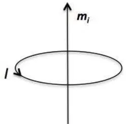
Figure 2.1: Magnetic dipole momentmi resulting from atomic current,I.

Each atomic current is a tiny closed circuit and therefore, a magnetic dipole mi could be

assigned to each atomi, as schematically shown in Fig. 2.1. The magnetic properties of matter are characterized by the macroscopic quantity, calledmagnetization, as

M= lim

∆v→0 1

∆v !

i

mi (2.1)

where∆vis the volume element, in which the magnetic dipole moments are vectorially summed up. It depends on both the individual magnetic moments of the atoms and how they interact with each other and is measured inAmperes per Meter in SI and emu/cm3 _{in cgs. It should}

(17)

be mentioned that for the purposes of this work we do not specifically use any microscopic description of the magnetic moments. We only use the macroscopic magnetization defined in Eq. 2.1.

The equation relating the applied magnetic fieldHand the magnetic induction,Bis (in SI unites)

B= µ₀(H+M) (2.2)

whereµ0is the permeability of free space and is a measure of the amount of resistance encoun-tered when forming a magnetic field in vacuum. It has an exact (defined) value ofµ0 =4π×10−7

Newtons per Ampere squaredin the SI systems.

Depending on the configuration of the electrons in the outermost shell of the atomic or-bitals, the reaction of the material to the external magnetic field, can change. If the valence shell of the atom is filled, then the atom does not have any net magnetization since the mag-netic fields from two paired electrons cancel each other and the net magnetization of the atom sums up to zero anddiamagneticeffect is observed in such materials. If an electron in the va-lence shell does not pair up with another electron, then each atom will have a net magnetization and this changes the magnetic properties of the material and how it reacts to an external mag-netic field. In such materials, eitherparamagnetismorferromagnetismis observed depending on the strength of the interaction among neighbouring magnetic moments.

2.1 Susceptibility, Permeability and Hysteresis

Knowing M is not enough to understand the magnetic properties of the material [60]. It is essential to have a relationship between B andH or, equivalently betweenM and one of the magnetic field vectors. This relationship depends on the nature of the magnetic material and is usually obtained from experiments. The ratio of the magnetization to the applied magnetic field is called the susceptibility, and it is not necessarily a scalar quantity. This means that the the magnetization produced in the material by applying the magnetic field,H, might not be in the direction ofH. In general the susceptibility,χi j, is defined as a second rank tensor

Mi =

!

j

χi jHj (2.3)

It shows how responsive a material is to an applied magnetic field. The ratio of the magnetic induction to the applied magnetic field is called permeability. To describe permeability in anisotropic media, a permeability tensor,µ_{i j}, is needed, which is defined as

Bi =

!

j

µi jHj, (2.4)

It indicates how permeable (penetrable) the material is to the magnetic field. A material which has higher amount of magnetic flux in it, has a higher permeability.

(18)

2.1. S, P H 7

Figure 2.2: Magnetization curve for typical paramagnetic and diamagnetic materials.

is negative and permeability is slightly less than one. For paramagnetic material the slope is positive and permeability is slightly greater than unity, as illustrated in Fig. 2.2.

Figure 2.3 shows the magnetization curve for ferromagnets. First of all, in ferromagnets permeability and susceptibility are much larger than dia- and paramagnets. A much larger magnetization is obtained by applying a much smaller external field. This is apparent from the rough values [60] denoted on the M and H axes in Figs. 2.2 and 2.3. Second, above a certain applied field, the magnetization converges to a constant value, the saturation magnetization. Finally, decreasing the field to zero does not reduce the magnetization to zero. It takes a magnetic field in the opposite direction to remove the magnetization. This phenomenon is calledhysteresis.

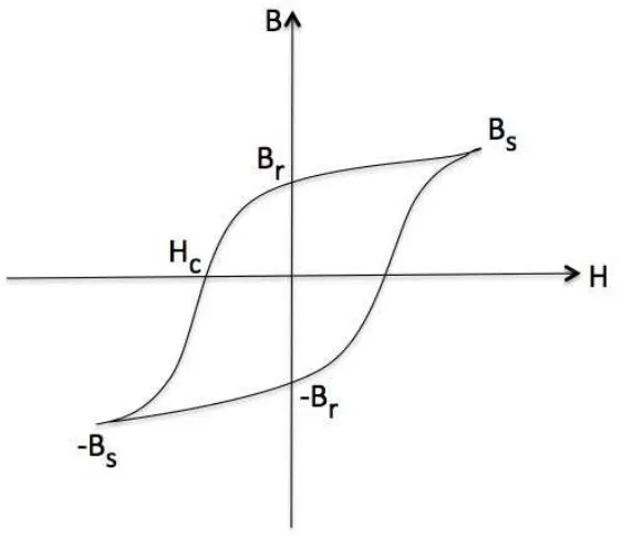
In fact, ferromagnets continue to show interesting behaviour when the fieldHis reduced to zero and then reversed in direction. The graph ofBorMversusHwhich shows the behaviour of ferromagnets in such a process is called ahysteresis loop. Considering the process shown in figure 2.4, the material starts in an unmagnetized state, at the origin. The magnetic induction follows the curve from 0 toBs, as the field is increased in the positive direction.Bcontinues to

increase even after the magnetization saturates, becauseB = µ0(H+M). WhenHis reduced to zero after saturation, the induction decreases fromBstoBr.

The magnetization left behind after an external magnetic field is removed, is called rema-nence. The reversed field required to reduce the induction to zero is called coercivity, Hc.

When the reversedHis increased further, saturation is achieved in the reverse direction. Both tips represent magnetic saturation and there is inversion symmetry about the origin.

(19)

Figure 2.3: Magnetization curve for typical ferromagnetic materials.

and inductors that need to operate at highACfrequencies. On the other hand if the coercivity is high, then a large magnetic field is required to demagnetize the magnetic material. Such materials are ideal as permanent magnets.

2.2 Diamagnetism

Diamagnetism is the result of Lenz’s law in atomic scale1_{. When a magnetic field is applied,} the atomic currents are modified in such a way that they tend to weaken the effect of this field, so the induced magnetic moments are directed opposite to the applied field. That is the reason why the slope of the curve for diamagnets in Fig. 2.2 is negative.

Diamagnetic effect occurs in all atoms even those in which all electron shells are filled and so have a zero net magnetic moment. In fact, it is such a weak phenomenon that only those atoms that have no net magnetic moment are classified as diamagnetic. In other materials, the net magnetic moment introduces much stronger interactions and the diamagnetic effect is negligible comparing to those interactions.

If a container of a diamagnetic material, such as bismuth, is suspended in a non-uniform magnetic field, it will swing away from the high field region, to decrease the induced magneti-zation energy inside it.

1_{Lenz’s law states that the induced current is in such a direction as to oppose the change of flux through the}

(20)

2.3. P 9

Figure 2.4: Hysteresis loop for a ferromagnetic material

2.3 Paramagnetism

Paramagnetic effect can be observed in materials that have a net magnetic moment. First, the orbital motion of each electron in an atom or molecule can be described in terms of a magnetic moment. Second, it is known that the electron has an intrinsic property called spin, and an intrinsic magnetic moment associated with this spinning charge. Each molecule then, has a magnetic moment which is the vector sum of orbital and spin moments from various electrons in the molecule.

Langevin theory of paramagnetism explains the paramagnetic effect and the temperature dependence of susceptibility [60]. In paramagnetic materials, magnetic moments are only weakly coupled to each other and so thermal energy causes random alignment of the magnetic moments. When an external magnetic field is applied, the moments start to align with the field. Suppose that a magnetic moment has an angleθwith the applied fieldH. In equilibrium at temperature T, the probability that the magnetic moment has an energyE, is given by the Boltzmann distribution:

e−E/kBT ₌ _em·H/kBT ₌_emHcosθ/kBT _(2.5)

Here,kBis the Boltzmann’s constant andmandHare the magnitudes of the respective fields.

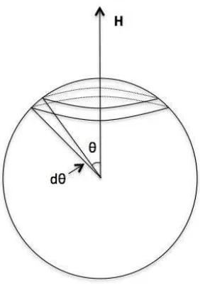
The number of moments having an angle betweenθandθ+dθwith respect toHis proportional to the fractional surface area of a surrounding sphere,dA=2πr2_sin_θ_d_θ_{, depicted in Fig. 2.5.}

(21)

Figure 2.5: Fractional area, dA, confined by the angledθ

p(θ)= e

mHcosθ/kBT_sin_θ_d_θ

"π

0 emHcosθ/kBTsinθdθ

(2.6)

where the factors of 2πr2 _{cancel out. Each moment contributes an amount}_m_cos_θ_{to the total} magnetization parallel to the magnetic fieldM

M=Nm< cosθ >= Nm

# π

0

cosθp(θ)dθ

=Nm

"π

0 e

mHcosθ/kBT_cos_θ_sin_θ_d_θ

"π 0 e

mHcosθ/kBTsin_θd_θ

(2.7)

Evaluating the integrals gives:

M= Nm$coth%mµ0H

kBT

&

− kBT mµ0H

'

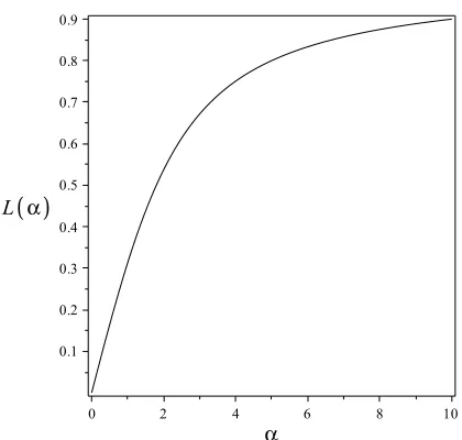
= NmL(α) (2.8)

whereα= mH/kBT andL(α) =coth(α)−1/αis called the Langevin function. L(α) is plotted

in Fig. 2.6. Asαincreases,L(α) approaches its maximum, andMapproachesNm. Increasing

αcorresponds to increasingHor decreasing the temperature which results in alignment of the spins with the applied magnetic field.

To find the susceptibility, we first Taylor expand the Langevin function around zero [60]:

L(α)= α

3 −

α3

45 +... (2.9)

(22)

2.4. F 11

Figure 2.6: Langevin function,L(α), used to describe the dependence of the susceptibility on temperature in paramagnetic materials

M= Nmα

3 =

Nµ0m2 3kB

H

T (2.10)

This gives the susceptibility:

χ= M

H =

Nµ₀m2 3kBT

= C

T (2.11)

whereC = Nm2_/₃_k

B. This isCurie’s law, which states that the susceptibility of a paramagnet

is inversely proportional to the temperature.

2.4 Ferromagnetism

There are some paramagnetic materials that do not follow Curie’s law, but instead follow the

Curie-Weisslaw:

χ= C

T ₋θ (2.12)

where θ is a constant, with the dimensions of temperature. Paramagnetic materials which follow the Curie-Weiss law undergo aspontaneous orderingand become ferromagnetic below some critical temperature,TC, which for all practical purposes is equal toθ. WhenT = θthe

(23)

molecular field, which does not vanish in the absence of an external magnetic field and results in the alignment of the magnetic moments in the absence of an applied field.

Weiss was able to explain the Curie-Weiss law i.e., Eq. 2.12, by assuming that the intensity of the molecular field is directly proportional to the magnetization

Hw =γM (2.13)

whereγis called themolecular field constant. Therefore, the total field would be:

Htot =H+Hw (2.14)

ReplacingHtotin the Curie susceptibility, Eq. 2.11, results in,

M H+γM =

C

T (2.15)

which gives,

χ= M

H =

C

T −Cγ =

C

T −θ (2.16)

which is the Curie-Weiss Law. θ = Cγis a measure of the strength of the interaction and is a property of the material.

2.4.1 Spontaneous magnetization

Using Weiss’ theory, we could see how spontaneous magnetization occurs. As discussed in section 2.3, the Langevin theory of paramagnetism tells us that the magnetization is given by Eq. 2.8.

Let us consider a sample in which each atom has a net magnetic moment. Based on the Langevin theory of paramagnetism, the magnetization of the material increases with increas-ing the applied magnetic field at constant temperature. The solid line in Fig. 2.7, is a plot of magnetization as a function ofα. Next, we assume that the only field acting on the material is the Weiss molecular fieldHw. InsertingH=Hwin the relation forαgives:

α= mHw

kBT

= mγM

kBT

(2.17)

which gives [60]:

M= %kBT

mγ

&

α (2.18)

Thus, the magnetization is a linear function ofα, with the slope proportional to temperature. The dotted and dashed lines in Fig. 2.7 are plots of this equation for T = TC and T < TC,

respectively.

(24)

2.4. F 13

Figure 2.7: Spontaneous magnetization in ferromagnetic materials.

increases, the slope of the line also increases and it intersects with the Langevin function at a smaller spontaneous magnetization.

AtT = TC, the only solution is at the origin, meaning that there is no spontaneous

magne-tization. As the temperature is decreased, the spontaneous magnetization increases smoothly, which is in agreement with the fact that paramagnetic to ferromagnetic transition is a continu-ous phase transition, as will be discussed in Chapter 4.

The essential aspects of ferromagnetism are illustrated by the implications of the following experimental facts [36]:

It is possible to change the overall magnetization of a suitably prepared ferromagnetic specimen from an initial value of zero (in the absence of an applied magnetic field) to a satu-ration value of the order of 1000 gauss, by the application of a field whose strength may be of the order of 0.01 oersteds.

The statement above contains two significant observations:

(a) It is possible in some cases to attain saturation magnetization by the application of a very weak magnetic field.

(b) It is possible for the magnetization of the same specimen to be zero in zero (or nearly zero) applied field.

(25)

increase the magnetization of a paramagnetic salt such as ferrous sulfate, by about 10−6_gauss, as compared with 103 _{gauss in the ferromagnetic specimen. The small e}_ff_{ect in the case of} the paramagnetic salt is known to be caused by thermal fluctuations of magnetic moments. In the paramagnetic salt effectively only one magnetic field in 109 _{is oriented by the field of} 0.01 oersted, so the distribution of the magnetic moment directions remains random. This high degree of randomness is a result of thermal fluctuations in a system where the magnetic moments are independent, without important mutual interaction.

Weiss pointed out that the randomness caused by thermal agitation could be largely cir-cumvented if one postulated in ferromagnetic materials the existence of a powerful internal molecular field, which is a mutual interaction between electrons which would tend to line up the magnetic moments parallel to one another.

The required magnitude for the Weiss molecular field may be estimated. At the Curie temperature,Tc, the thermal energykBTcof an electron spin is of the same order of magnitude

as the interaction energyµHwof the magnetic momentµof an electron acted on by the effective

molecular fieldHw:

kBTc ≈ µHw (2.19)

so that

Hw ≈ kBTc

µ ≈

10−16₁₀3 10−20 ≈10

7_oersteds _(2.20)

This is a very powerful effective field. It is about twenty times more intense than any actual magnetic field produced in a laboratory. At temperatures belowTc, the effect of the molecular

field outweighs the thermal fluctuation energy and the specimen is accordingly ferromagnetic. It is known that the origin of the molecular field lies in the quantum mechanical exchange force [36] and the ordinary magnetic moment interaction between electrons is much too weak to account for the molecular field. The magnetic field at a lattice point, arising from the mag-netic moment of a neighbouring electron is of the order of:

H ≈ µ

r3 ≈

10−20

(2_×10−8₎3 ≈10

3_oersteds _(2.21)

which is smaller than the effective molecular fieldHwby a factor of the order of 10−4.

2.5 Domain Theory

In the previous section we saw how the existence of the powerful Weiss molecular field enables saturation magnetization to be obtained. How do then we explain statement (b) above, that it is possible for the magnetization to be zero in zero applied field? It seems at first sight contradictory, in view of the 107oersted molecular field, to suppose that a 10−2_{oersted applied} field can alter the magnetic moment of the specimen by an appreciable amount [36].

(26)

2.6. T  D 15

in the value of the resultant magnetic moment of the specimen under the action of an applied field may be imagined to take place by an increase in the volume of the domains which are favourably oriented with respect to the field at the expense of unfavourably oriented domains; or by rotation of the direction of magnetization towards the direction of the field, Fig. 2.8.

Figure 2.8: Schematic domain arrangement in a ferromagnetic material and magnetization of the sample by domain growth and domain rotation.

In weak fields the magnetization changes usually proceed by means of domain boundary displacements so that the domains change in size. In strong fields the magnetization changes by means of rotation of the direction of magnetization.

2.6 The origin of Domains

There are a number of different contributions to the total magnetic energy of the ferromag-netic material. The formation of domains allows the minimization of the total free energy

which consists of: exchange energy, magneto-static energy, magnetocrystalline (anisotropy) and magnetostriction (magnetoelestic) energies.

2.6.1 Exchange Energy

Heisenberg showed that the Weiss molecular field could be explained using a quantum

me-chanical treatment of the many-body problem [60].

Looking at the quantum mechanical calculation for the energy of the helium atom, which has two electrons and provides a simple example of the many-body Hamiltonian shows that there is a term ofelectrostatic originin the energy of interaction between neighbouring atoms that tends to orient the electron spins parallel to each other. This term is called theexchange integraland does not have a classical analog [60].

The exchange interaction is a result of thePauli exclusion principle, which states that no two identical fermions (particles with half-integer spins) may occupy the same quantum state simultaneously [58]. For example, no two electrons in a single atom can have the same four quantum numbers. Ifn,l,mlare the same, thenmsmust be different such that the electrons have

(27)

state. But this results in a spatial overlap of the two electrons which increases the electrostatic Coulomb repulsion. On the other hand, if they have parallel spins, they must occupy different states and will minimize any unfavourable repulsion interaction.

If two atoms i and j have spins of Si and Sj, then the exchange energy between them is

given by [36]

Eex =−JexSi·Sj =−jexSiSjcosφ (2.22)

where Jex is a particular integral, called theexchange integral, which occurs in calculation of

the exchange effect and φis the angle between the spins. If Jex is positive,Eex is a minimum

when the spins are parallel and a maximum when they are anti-parallel, which is the case for ferromagnetic materials.

Figure 2.9: Reduction of magnetostatic energy by domain formation. In (a) the external de-magnetizing field is big. In (b) the block is divided into domains to decrease the dede-magnetizing field and therefore the magnetostatic energy. In (c) the triangular domains at the top and bottom of the sample allow the magnetostatic energy to be completely zero, as they are paths by which the flux can close on itself.

2.6.2 Magnetostatic Energy

(28)

2.6. T  D 17

configuration does not have any magnetic poles at the surface of the sample, and accordingly the demagnetizing field is zero in this configuration.

2.6.3 Magnetocrystalline Energy

The anisotropy energy or the magnetocrystalline energy is minimized when the magnetization aligns in certain definite crystallographic axes, which are called directions of easy

magneti-zation. Measurements show that in iron, for example, the saturation magnetization can be

achieved with quite low fields, of order of a few tens of oersteds in the direction of easy mag-netization<100>2, while it takes high fields, of the order of several hundred oersteds to saturate iron in<111>direction which is accordingly called thehard direction of magnetization.

Figure 2.10: Domain configuration that minimizes the magnetocrystalline energy in a uniaxial crystal.

To minimize the magnetocrystalline energy, the domains will form so that their magneti-zation is along the easy direction. For a uniaxial crystal (like hexagonal crystals of cobalt) the domain structure is particularly simple, as seen in Fig. 2.10. The domains of closure form when the material has easy axes that are perpendicular to each other. In such materials, this configuration is favourable because it eliminates the magnetostatic energy, without increasing the magnetocrystalline anisotropy energy [60].

2_{The orientation of a plane is given by a vector normal to the plane. There are reciprocal lattice vectors normal}

(29)

The origin of the magnetocrystalline anisotropy is thespin-orbit coupling[58]. Because of this coupling, the orbit of the electrons needs to be reoriented when the spin aligns along an applied magnetic field. However, the orbit is strongly coupled to the lattice. This explains the resistance against the rotation of spin, due to the magnetocrystalline anisotropy.

2.6.4 Magnetostriction Energy

The change in the dimensions of a ferromagnetic material in the presence of an external mag-netic field is called magnetostriction effect [14]. The fractional change in length∆l/lis simply a strain, which is different from the strain caused by an applied stress. The magnetically induced strain, which can be negative or positive, is given by:

λ= ∆l

l (2.23)

Magnetoscriction is described using a quantity called the magnetistrictive coefficient, L, and is defined as the fractional change in length of the sample as the magnetization of the material increases from zero to the saturation value. It is a very small quantity, of order of

L∼ 10−5 _{for magnetic materials such as Iron, Nickel and Cobalt [9].}

In iron, the magnetostriction causes the domains of closure in Fig. 2.9-c to try to elongate horizontally, and the long vertical domains try to elongate vertically. Since both elongations can not happen at the same time, a change in the length of the substance happens [60]. An elastic strain energy term is added to the total free energy, to explain this effect. This elastic energy is proportional to the volume of the domains of closure and can be lowered by reducing the size of closure domains, which results in smaller domains. This increases the exchange energy. Thetotal free energyis minimized by a compromised domain arrangement such as that shown in Fig.2.11

Magnetostriction effect is also due tospin-orbit coupling. The mechanism of magnetostric-tion is schematically shown in figure 2.12. The picture shows a secmagnetostric-tion through a row of atoms in a crystal. Below the Curie temperature, they orient about the easy axis (horizontal axis in this picture) due to the spin-orbit coupling [14].The change in length of the specimen occurs when the specimen is exposed to strong fields. Then the spins and electron orbitals would ro-tate to be parallel to the direction of the field and the domain of which theses atoms are a part would experience a strain∆l/l.

2.7 Coercive Force

(30)

2.7. CF 19

Figure 2.11: A domain arrangement that reduces the total energy which is the sum of of exchange, magnetostatic, magnetocrystalline and domain wall energy.

When a magnetic domain boundary crosses the imperfection, the poles will be removed by formation of closure domains and therefore the magnetostatic energy could be eliminated. A local energy minimum occurs in the intersection of the magnetic domain boundary and the crystal imperfection. This is a local minimum, and energy is needed to move the domain boundary and pass it over the imperfection. This energy is provided by the applied magnetic field. Eventually the applied field will remove all domain walls and produce a single domain.

When the magnetic field is removed, the dipoles rotate back to their easy axis. Now the domain walls should move back to their initial state. However, the demagnetizing field is much weaker than the applied external magnetic field and is not strong enough to overcome the energy barriers and pass the magnetic domains across the imperfections. Therefore, the sample remains partially magnetized when the external magnetic field becomes zero. The

(31)

(32)

Chapter 3 Solidification and the Origin of Grain

Structure

In this chapter, the classical approach to the solidification of a pure liquid (the Stefan prob-lem), the equilibrium phase behaviour of binary mixture and different kinetics observed in the phase transition process (nucleation and spinodal decomposition) are considered. The discus-sion about the solidification is provided, as a background to understand the physics behind the crystallization from an undercooled melt in the PFC simulations (Chapter 6). Discussions regarding the equilibrium phase diagram of the binary mixture provide the basis to understand the common tangent construction used in Chapter 8 to calculate the phase diagram of the Mag-netic PFC model. Finally, the differently oriented grains resulting from nucleation at different sites of the system are considered and the experiments on the dependence of magnetic hardness on grain size are explained in Section 3.3. The results of the simulations, using the Magnetic PFC model to reproduce these experimental data are reported in Chapter 9.

The process of crystal growth from a liquid phase is referred to as solidification [43]. In general, complex patterns can be produced in a solidification process, which are controlled by the external conditions at which a crystal is growing. A natural example of crystal growth is the formation of snowflakes, which have dendritic (tree like) microstructure. These structures are controlled by the temperature and humidity and the concentrations of various air pollutants. A typical dendritic microstructure, developed by immersing a crystalline seed in its undercooled melt, is shown in Fig. 3.1.

Dendritic structure also occurs in solidification of alloys. The patterns are very sensitive to growth conditions and material parameters. In these microstructures, defects and chemi-cal inhomogeneities, which have been formed during the solidification process, determine the mechanical, thermal, electric and magnetic properties of solids. For example yield strength of a polycrystal varies as the inverse square of the average grain size [19]. Accordingly, under-standing the solidification process is very important since it forms the basis for controlling the microstructure and therefore the macroscopic properties and behaviour of alloys.

(33)

Figure 3.1: Primary dendrite of succinonitrile (a transparent crystal with cubic symmetry) growing in its undercooled melt. Note the smooth paraboloidal tip, the secondary sidebranch-ing oscillations emergsidebranch-ing behind the tip and the beginnsidebranch-ing of tertiary structure on the well-developed secondaries [44] .

3.1 Solidification of a pure liquid

The simplest solidification process is the solidification of a pure substance from its melt, for example, the freezing of ice from water. For a pure substance, solidification is completely governed byheat flow. The rate of solidification at any point is controlled by how fast the latent heat released, can be transferred into the bulk or removed at the boundaries [43]. Solidification of a material with a melting point above the ambient temperature will take place once some of the solid has formed.

Considering the solidification in a container or mould, the heat effectively is being trans-ferred to the ambient environment via the mould. The heat flux from the hot melt to the sur-rounding material allows the liquid to cool and to transform to solid and the solid to cool to reach the temperature of the surrounding medium.

In the case of a pure material, the basic element in the mathematical problem of predicting the motion of the solidification interface is a diffusion field, i.e., the temperature T which satisfies the diffusion equation

∂T

∂t =DT∇

2_T _(3.1)

where DT is the thermal diffusion constant. We need to write Eq. 3.1 for the liquid and solid

phases, with different values of diffusion constants (DT and D(_T). We also need the condition

of heat conservation at each point on the moving interface:

Lvn =

$

D(_Tc(_p(_∇T)_solid₋DTcp(∇T)liquid

'

(34)

3.2. K 23

whereLis the latent heat per unit volume of the solid,cp andc(pare the specific heats per unit

volume of the liquid and solid, respectively;vn is the normal velocity of the interface and ˆnis

the normal vector of the interface. Thus, the left-hand side is the rate at which heat is generated at the boundary and the right-hand side is the rate at which this heat flows into the bulk phases on either side.

To describe the motion of the solidification front, this model also needs a thermodynamic boundary condition at the interface. The simplest choice would be that the temperature along the surface of the interface must be equal to the bulk melting temperature. With this condition we reach to a relatively tractable mathematical problem, theStefan problem[43]. However this simple condition omits the effect of surface tension which is a crucial force in pattern formation problems.

In fact, for any solid/liquid bulk of volume V which is enclosed by an interface of area A, there is an excess interface energy which is required for its creation. So in inhomogeneous systems, part of the system which has a higher A/V ratio, has a higher energy and therefore less stable relative to a part which has a lowerA/V ratio. The relative stability can be related to the equilibrium temperature of the two phases (melting point).

The correct form of the thermodynamic boundary condition is:

Tinter f ace = TM(1−(γK/L))−β(vn) (3.3)

where γ is the liquid-solid surface tension, K is the curvature of the interface, defined to be positive for a convex solid and TM is the melting temperature of the bulk. The term β(vn)

is a function of the normal interface velocity to correct for kinetic effects. A linear function

β =β0vn would be accurate for a rough interface. Equation (3.3) is called theGibbs-Thomson

relation [43], which describes the change in melting point (Tinter f ace−TM) due to the curvature

effect. Equations (3.1), (3.2) and (3.3) completely specify the model of solidification of a pure substance.

A useful analysis to study the stability of a particular pattern in the process of solidification is theMullins-Sekerka Instability[43]. The basic idea in this method is to introduce a pertur-bation in the original interface shape and to determine whether this perturpertur-bation will grow or decay [49].

Using the linear stability analysis [43], it is observed that simple shapes such as planes, spheres, cylinders, etc., are unstable under certain commonly encountered conditions and more complicated patterns are formed. This instability occurs because on the one hand, diffusion kinetics favours as large a surface area as possible so that latent heat can be dissipated more rapidly; on the other hand the surface tension increases when the ratioA/V increases. It is the interplay between these two effects which produces the complex growth patterns observed in nature.

3.2 Kinetics

(35)

under-standing of the process, we need to look at the kinetics of the process by which the phase transition happens.

A change in temperature of a liquid that is so rapid that the state of the system immediately after the change is still liquid, is called a quench. After the system is quenched, the under-cooling, i.e., the difference between the temperature of the undercooled liquid and the melting temperature will drive the system to solid phase, to minimize the free energy.

3.2.1 Phase diagram

In this section a brief description on the phase diagram of a binary liquid mixture is provided. The discussions of this section are based on [34] and help us to understand the phase behaviour of a system with two phases that are different in concentration or density, in the temperature-concentration plane. This produces the basic framework of phase diagram calculation of the Magnetic PFC model in Section 8.2.

In order to understand the kinetics of phase transitions, we look at a simple example: The situation in which two liquids of types Aand B in aclosed container are miscible in all pro-portions at high temperature, but separate into two distinct phases (A-rich zones and B-rich zones) when the temperature is lowered. To calculate the equilibrium states of the system as a function of the temperature and composition, i.e., thephase diagram, the free energy of mixing is estimated using the mean field theory. The mean field assumption here is that a given site of the system haszφA (A) neighbours andzφB (B) neighbours whether the site is occupied byAor Bmolecules.

The order parameter is taken to be the volume fraction ofAmolecules,ηA, which is defined

to be the volume of Amolecules divided by the total volume of the system. If the system is incompressible, ηB = 1−ηA. If we know the volume fraction of A, then the volume fraction

ofBcan be calculated; therefore, from here on we assume all volume fractions refer toA. The details of the calculation can be found in [34]. Here, we only consider the main results of the calculation which enables us to understand the phase diagram.

The free energy of mixingFmixis

Fmix = FA+B−(FA+FB) (3.4)

whereFA+Bis the free energy of the system ifAandBare mixed in a single container,FAis the

free energy of the system containingAmolecules only andFB is the free energy of the system

containingBmolecules only.

It is shown in [34] that the free energy of mixing is equal to

Fmix kBT

=ηlnη+(1₋η) ln(1₋η)+χη(1₋η) (3.5)

whereχis the energy change in units ofkBT when a moleculeAis taken from an environment

of pure A and put into an environment of pure B. It expresses the strength of the energetic interaction between the Aand B components. It is temperature dependent and varies as 1/T

(36)

3.2. K 25

Figure 3.2: Plots of the free energy of mixing, Eq. 3.5 for different values ofχ. The system has one minimum for the interaction parameters χ < 2, at a volume fraction ofη = 0.5. This means that the mixture is miscible, regardless of the initial proportions ofAandB. Forχ _≥ 2 the free energy has two minima and a maximum atη=0.5.

If we plot the free energy curve as a function of the volume fractionη, for different values ofχ (Fig. 3.2), we see that forχ < 2 the curve has a global minimum at ηA = ηB = 0.5. For χ_≥2 the curve has two minima, and a maximum atηA = ηB =0.5.

To understand whether a phase-separated phase is stable or the mixture, we need to calcu-late the free energy of the phase-separated system,Fsep, and compare it with that of the mixed

system,Fmix. We consider a volume,V0, of mixture whose starting volume fraction isη0. If the mixture separates into a region of volume, V1, with volume fraction, η1, and a region of volume,V2, with volume fraction,η2, then we haveη0V0 =V1η1+V2η2. This is due to the fact that the system is closed and the total number ofAandBis conserved. Thus we can write

η0 =α1η1+α2η2 (3.6)

whereα1andα2are the relative proportions of the two phases and

α1+α2= 1 (3.7)

The free energy of the phase-separated system,Fsep = α1Fmix(η1)+α2Fmix(η2), can be written as

Fsep =

η0−η2

η1−η2

Fmix(η1)+

η1−η0

η1−η2

Fmix(η2) (3.8)

(37)

to the value of this straight line at the volume fractionη0. For a concave curve this free energy is higher than the free energy, Fmix(η0), for all values of η1 andη2. This situation is shown in Fig. 3.3-a. This means that for allχ <2 values or equivalently for all temperatures greater than a critical temperature, the mixture is miscible, regardless of the initial proportions ofAandB.

If there is any region of compositions for which the free energy curve is convex, then there are some initial compositions that can lower the free energy by phase separation. Such regions can be found in the free energy curve shown in Fig. 3.3-b. The free energy of the phase-separated system, is evaluated by calculating the value of the straight line “1”, joining two compositionsη1 andη2, atη0. It can be observed in the figure that it is less than the free energy of the mixed system atη0. Thus, at this temperature there exist initial compositions that are unstable with respect to phase separation.

The limiting compositions, η1, and η2, that separate the regions of concavity of the free energy from the regions of its convexity are the compositions that are joined by acommon tan-gent, line “2”, and are known as thecoexistingcompositions. If we increaseχor decrease the temperature,the composition range enclosing the unstable phase increases. Thus in the phase diagram the region enclosed by the coexistence line should become wider as the temperature is decreased.

(a) The plot ofFmixforχ=1 (b) The plot ofFmixforχ=2.6

Figure 3.3: The free energy of mixing for different values of the interaction parameter, χ or equivalently at different temperatures. In (a), the free energy of mixing is concave and has one global minimum. Thus the value of Fsep(η0) is greater than Fmix(η0) for all compositionsη1 and η2 and the mixture is stable at all proportions. In (b), χis increased or correspondingly the temperature is decreased. Fmix has both regions of convexity and concavity. Line “1” in

(38)

3.2. K 27

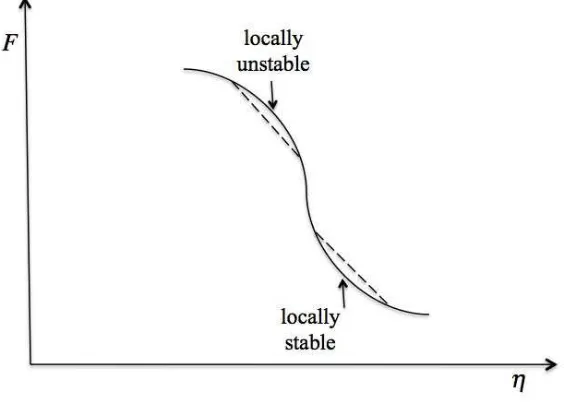
Figure 3.4: The free energy of mixing as a function of the composition. This figure schemati-cally shows a composition in which the system is loschemati-cally stable (metastable) and a composition in which the system is unstable.

For the compositions that are within the coexistence curve there is another distinction: the curvature of the free energy in this region might be either positive or negative. As shown in Fig. 3.4 the system might be either locally stable or locally unstable although it is globally unstable. This means that there exist some compositions in this region that are unstable with respect to small fluctuations in composition (locally and globally unstable). Any small fluctu-ation in composition will cause a phase separfluctu-ation. On the other hand there exist compositions where the system is locally stable with respect to separation into two coexisting phases al-though it is globally unstable. These are the compositions at which the system is in the state of

metastability. In this case, if the fluctuation is big enough to overcome the free energy barrier, the system will phase separate. But if the fluctuation is small the system will not ”see” that it is in the globally unstable phase and will not phase separate. The limit of local stability is determined by the condition thatd2_F_/_d_η2₌_{0 and defines the}_{spinodal line}_.

With this information about the free energy, we can determine the equilibrium phase of a liquid-liquid mixture at a particular temperature and density, i.e., we can calculate thephase diagram. Figure 3.5 shows the phase diagram of such systems. It can be observed in the figure that at a certain point on top of the coexistence line, the stable phase and unstable phase are indistinguishable. This point is the thecritical pointof the phase diagram. Above this point, it is possible to pass to different volume fractions without going through a coexistence region.

As shown in Fig. 3.5, if a mixture having a particular initial value of composition, η0, is quenched down below the coexistence line or equivalently if χ is increased, it will phase separate to regions with compositionη1 (B-rich regions) and regions with compositionη2 (A-rich regions).

(39)

Figure 3.5: The phase diagram of a binary liquid mixture. The horizontal axis is the volume fraction of the A component. If we prepare the system at an initial volume fraction, η0, and quench the system to the unstable region of the phase diagram, it will separate into two phases with volume fractionsη1 (B-rich) andη2(A-rich).

N = N1+N2 is a constant and thatη0 = α1η1+α2η2, i.e., Eq. 3.6. Minimizing with these two constraints gives us a set of equations that is the mathematical formulation for the common tangent construction [56]

µ = ∂Fmix

∂η1

= ∂Fmix

∂η2

(3.9)

µ = Fmix(η1)−Fmix(η2)

η1−η2

(3.10)