Design optimization considering variable thermal mass, insulation, absorptance of solar radiation, and glazing ratio using a prediction model and genetic algorithm

(1)

sustainability

Article

Design Optimization Considering Variable Thermal

Mass, Insulation, Absorptance of Solar Radiation,

and Glazing Ratio Using a Prediction Model and

Genetic Algorithm

Yaolin Lin1,*, Shiquan Zhou1, Wei Yang2and Chun-Qing Li3

1 _{School of Civil Engineering and Architecture, Wuhan University of Technology, Wuhan 430070,}

China; [email protected]

2 _{College of Engineering and Science, Victoria University, Melbourne 8001, Australia; [email protected]}

3 _{School of Engineering, RMIT University, Melbourne 3000, Australia; [email protected]}

* Correspondence: [email protected] or [email protected]

Received: 18 December 2017; Accepted: 24 January 2018; Published: 29 January 2018

Abstract:This paper presents the optimization of building envelope design to minimize thermal load and improve thermal comfort for a two-star green building in Wuhan, China. The thermal load of the building before optimization is 36% lower than a typical energy-efficient building of the same size. A total of 19 continuous design variables, including different concrete thicknesses, insulation thicknesses, absorbance of solar radiation for each exterior wall/roof and different window-to-wall ratios for each façade, are considered for optimization. The thermal load and annual discomfort degree hours are selected as the objective functions for optimization. Two prediction models, multi-linear regression (MLR) model and an artificial neural network (ANN) model, are developed to predict the building thermal performance and adopted as fitness functions for a multi-objective genetic algorithm (GA) to find the optimal design solutions. As compared to the original design, the optimal design generated by the MLRGA approach helps to reduce the thermal load and discomfort level by 18.2% and 22.4%, while the reductions are 17.0% and 22.2% respectively, using the ANNGA approach. Finally, four objective functions using cooling load, heating load, summer discomfort degree hours, and winter discomfort degree hours for optimization are conducted, but the results are no better than the two-objective-function optimization approach.

Keywords:design optimization; prediction model; thermal load; thermal comfort

1. Introduction

The energy consumption in building sector accounts for about one third of the primary energy consumption in the world [1]. About 40% of the total energy in the U.S. was consumed by buildings [2]. The building energy consumption in China is second only to the USA [1] and is increasing with the great demand for thermal comfort. Therefore, it is very important to design energy efficient buildings to minimize building energy consumption while maintaining or improving the indoor thermal comfort level.

The building energy demand can be alleviated through improved/optimized building design to reduce the thermal load of the buildings [3–5]. Thermal load and thermal comfort of buildings are affected by a number of factors, among which thermal mass (in particular the thickness of the concrete slab), insulation level, absorptance of solar radiation of the exterior walls/roof, and glazing ratio (also known as the window-to-wall ratio) are four factors that have important impacts [6]: (1) thermal mass can affect the fluctuation of the daily temperature inside the house; (2) insulation can affect the

(2)

Sustainability2018,10, 336 2 of 15

conduction heat gain/loss through the opaque envelope; and (3) the absorptance of solar radiation of the opaque envelope and the location and size of the windows can affect the solar heat gain.

Various approaches have been applied to improve building design through the consideration of thermal mass, insulation level, absorptance of solar radiation, and glazing ratio, and they have been studied at different levels of detail, e.g., uniform solar absorptance for all exterior walls [7–9], different solar absorptance for each external wall [10], one solar absorptance variable for the roof [8,11], uniform window size for all façades [5,7,9,12–17], different window sizes for each façade [18–27], uniform insulation level for exterior walls and roof [13,28], uniform external wall insulation level [17,22,29], one variable for external wall insulation and one variable for roof insulation [5,11,12,21,30–33], different insulation levels for each wall [34], and uniform thermal mass for all external walls [20,21,28,29]. By taking into account the building design variables and using optimization algorithms, the reduction on building energy consumption can be as much as 50% with thermal comfort improved by 1.5% [23].

So far, no literature has been found that has proposed a design optimization considering thermal mass, insulation level, absorbance of solar radiation for each exterior wall/roof, and glazing ratio for each façade at the same time. However, to achieve full potential of energy savings with improved thermal comfort in building design, all those variables deserve to be fully explored. Optimization on each of the parameters can result in improvement for the building performance (reduction of thermal load and discomfort degree hours). When one more parameter is added for optimization, further improvement can be achieved, which results in a greater reduction on thermal load and discomfort degree hours. As the number of design variables increases, the level of complexity to obtain optimal design solutions also increases. One way to solve this problem is to use parallel computing technology, e.g., the optimization time was reduced from almost 12 days to 4.4 h for the cases with 108 and 1016 possibilities when coupled optimization approach with simulation software [9], and from 118 h to 3 h with 48 processors using parallel computing for the case with six discrete variables [35]. The other way is to use an energy prediction model to characterize building behavior and then combine this with genetic algorithm, where most of the time was used to generate the sample data, e.g., it took three weeks to generate the results of thermal load and comfort level of 450 cases for two residential houses in Canada, and it took around 7 min to complete the optimization process which may take 10 years when using simulation software coupled with a genetic algorithm directly [20]. As parallel computing resources are not always available, the latter approach is adopted in this paper by developing prediction models to couple with genetic algorithms to find the optimal design solutions.

In this paper, different variables of thermal mass, insulation, absorbance of solar radiation are assigned for each exterior wall/roof, and the glazing ratios for each façade are considered separately. A total of 19 variables are considered, including five variables for concrete thickness, five variables for insulation thickness, five variables for the absorptance of solar radiation for each exterior walls/roof, and four variables for the window-to-wall ratio of each façade. In order to reduce the computation time, the Latin Hypercube Sampling Method is used to create the samples required to generate prediction models, and the commercial software, DesignBuilder (DesignBuilder Software Ltd, Stroud, Gloucestershire, UK) [36], is used to calculate the sub-hourly heating load, cooling load, and indoor air temperature to evaluate the thermal comfort condition. Two typical prediction models, multi-linear regression (MLR) model and an artificial neural network (ANN) model, are developed based on the sample data and coupled with a multi-objective genetic algorithm to find the optimal design solutions. The results from the two objective functions, namely, thermal load and annual discomfort degree hours, are also compared with the outcomes using the cooling load, heating load, summer discomfort degree hours, and winter discomfort degree hours as the objective functions for optimization.

(3)

a building with a high indoor thermal comfort level and low thermal load. The accurate modeling can ensure utilizing the least amount of materials to achieve optimal building performance. Optimal usage of material for different building components can be selected to achieve a minimum thermal load and discomfort degree hours, which is different from traditional design, and can improve the quality of construction project. This is coincidence with 3D printing technology where the material for each component can be tailored. It is expected that advancement of 3D house printing technology will make it possible for wide application in design practice in the future.

2. Optimization Approach

2.1. Formulation of the Problem

2.1.1. Objective Functions to be Optimized

The following two objective functions are used in this study to find the optimal building design, and they are described as follows:

Min f1(x), f2(x), x= [x1, x2· · ·, xn]. (1)

The first objective function is the annual thermal load, which was also investigated by [5,37]. The total building thermal load, calculated by DesignBuilder (DesignBuilder Software Ltd., Stroud, Gloucestershire, UK) [36], was composed of a cooling load and heating load:

f1(x) =QC(x) +QH(x). (2)

The second objective function is the total number of discomfort degree hours, which was proposed by Zhang et al. [38]. The total number of discomfort degree hours is composed of two parts. The first part is the cooling discomfort degree hours, which can be calculated as [37,38]:

Is(x) =∑8760i=1(ti(x)−tH) (if ti(x)>tH). (3)

where ti(x)is the indoor air temperature at time i; and tH is the higher limit temperature in the

thermal comfort range, taken as 26◦C according to the energy efficient building design standard JGJ134-2010 [39].

The second part is the heating discomfort degree hours, which can be calculated as [38]:

Iw(x) =∑8760_i=1(tL−ti(x))(if ti(x)<tL). (4)

where tLis the lower limit temperature in the thermal comfort range, taken as 18◦C according to

JGJ134-2010 [39].

The total number of discomfort degree hours is then calculated as:

f2(x) =Is(x) +Iw(x). (5)

2.1.2. Base Model

(4)

efficient building of the same size before further optimization is applied. The typical energy efficient building was built to meet the standard JGJ134-2010 [39] with K values of 0.974 W/m-K for the exterior walls, 0.592 W/m-K for the roof, and 3.835 W/m-K for the window, respectively. The thermal load of the energy efficient building is 36,301.50 kWh, while the one of the green building is 23,233.00 kWh.

Sustainability 2018, 10, x FOR PEER REVIEW 4 of 15

window, respectively. The thermal load of the energy efficient building is 36,301.50 kWh, while the one of the green building is 23,233.00 kWh.

Figure 1. Overview of the base building.

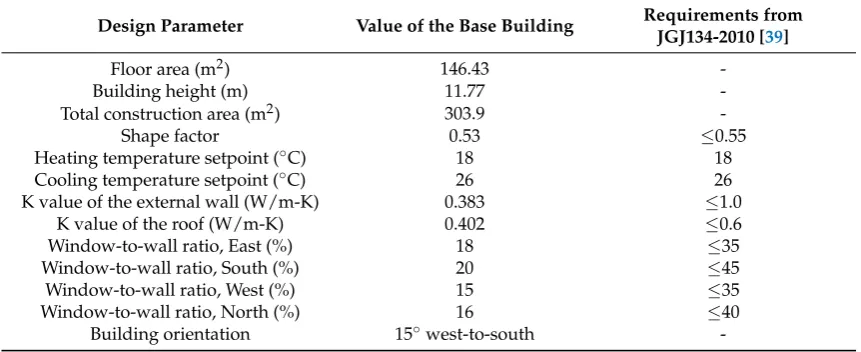
Table 1 lists the values of design parameters of the base building and the requirements from the energy efficient building design standard JGJ134-2010 [39]. It can be found that the K values of the external walls/roof and window-to-wall ratio far exceed the requirements from JGJ134-2010 [39].

Table 1. Values of the design parameters for the base building.

Design Parameter Value of the Base

Building

Requirements from JGJ134-2010 [39]

Floor area (m2_{) 146.43 -}

Building height (m) 11.77 -

Total construction area (m2_{) 303.9} _-

Shape factor 0.53 ≤0.55

Heating temperature setpoint (°C) 18 18

Cooling temperature setpoint (°C) 26 26

K value of the external wall (W/m-K) 0.383 ≤1.0

K value of the roof (W/m-K) 0.402 ≤0.6

Window-to-wall ratio, East (%) 18 ≤35

Window-to-wall ratio, South (%) 20 ≤45

Window-to-wall ratio, West (%) 15 ≤35

Window-to-wall ratio, North (%) 16 ≤40

Building orientation 15° west-to-south -

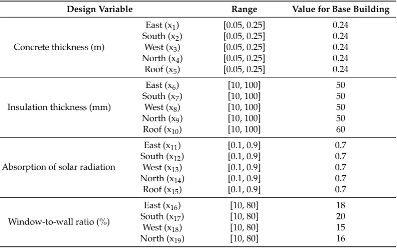
A total of 19 design variables are selected for study, which are concrete thickness, insulation thickness, and absorptance of solar radiation for each external wall/roof, and window-to-wall ratio for each façade. Table 2 lists the variable types and value ranges.

Figure 1.Overview of the base building.

Table1lists the values of design parameters of the base building and the requirements from the energy efficient building design standard JGJ134-2010 [39]. It can be found that the K values of the external walls/roof and window-to-wall ratio far exceed the requirements from JGJ134-2010 [39].

Table 1.Values of the design parameters for the base building.

Design Parameter Value of the Base Building Requirements from JGJ134-2010 [39]

Floor area (m2) 146.43

-Building height (m) 11.77

-Total construction area (m2) 303.9

-Shape factor 0.53 ≤0.55

Heating temperature setpoint (◦C) 18 18

Cooling temperature setpoint (◦C) 26 26

K value of the external wall (W/m-K) 0.383 ≤1.0

K value of the roof (W/m-K) 0.402 ≤0.6

Window-to-wall ratio, East (%) 18 ≤35

Window-to-wall ratio, South (%) 20 ≤45

Window-to-wall ratio, West (%) 15 ≤35

Window-to-wall ratio, North (%) 16 ≤40

Building orientation 15◦west-to-south

(5)

Table 2.Variable types and value ranges.

Design Variable Range Value for Base Building

Concrete thickness (m)

East (x1) [0.05, 0.25] 0.24

South (x2) [0.05, 0.25] 0.24

West (x3) [0.05, 0.25] 0.24

North (x4) [0.05, 0.25] 0.24

Roof (x5) [0.05, 0.25] 0.24

Insulation thickness (mm)

East (x6) [10, 100] 50

South (x7) [10, 100] 50

West (x8) [10, 100] 50

North (x9) [10, 100] 50

Roof (x10) [10, 100] 60

Absorption of solar radiation

East (x11) [0.1, 0.9] 0.7

South (x12) [0.1, 0.9] 0.7

West (x13) [0.1, 0.9] 0.7

North (x14) [0.1, 0.9] 0.7

Roof (x15) [0.1, 0.9] 0.7

Window-to-wall ratio (%)

East (x16) [10, 80] 18

South (x17) [10, 80] 20

West (x18) [10, 80] 15

North (x19) [10, 80] 16

The climatic information of Wuhan is listed in Table3.

Table 3.Climatic information.

City Latitude (◦)

Longitude (◦)

HDD18 (◦C·d)

CDD26 (◦C·d)

Average OAT

(◦C) Climatic Region

Wuhan 30.62 114.13 1501 283 16.7 Hot Summer & Cold

Winter Region

2.2. Optimization Framework

The optimization framework of this study is summarized in Figure2, and is divided into three steps. In the first step the simulation software obtained the thermal load and discomfort degree hours for a selected number of samples, which are generated based on the ranges of the 19 design variables as shown in Table2. In the second step the samples from the database is used to develop two prediction models, the MLR model and the ANN model. In the third step, the MLR model and the ANN model are used to couple with a multi-objective genetic algorithm to find the optimal solutions. Finally, the results of the optimal solutions based on different prediction models and objective functions are compared and discussed.

Table 2. Variable types and value ranges.

Design Variable Range Value for Base Building

Concrete thickness (m)

East (x1) [0.05, 0.25] 0.24

South (x2) [0.05, 0.25] 0.24

West (x3) [0.05, 0.25] 0.24

North (x4) [0.05, 0.25] 0.24

Roof (x5) [0.05, 0.25] 0.24

Insulation thickness (mm)

East (x6) [10, 100] 50

South (x7) [10, 100] 50

West (x8) [10, 100] 50

North (x9) [10, 100] 50

Roof (x10) [10, 100] 60

Absorption of solar radiation

East (x11) [0.1, 0.9] 0.7

South (x12) [0.1, 0.9] 0.7

West (x13) [0.1, 0.9] 0.7

North (x14) [0.1, 0.9] 0.7

Roof (x15) [0.1, 0.9] 0.7

Window-to-wall ratio (%)

East (x16) [10, 80] 18

South (x17) [10, 80] 20

West (x18) [10, 80] 15

North (x19) [10, 80] 16

The climatic information of Wuhan is listed in Table 3.

Table 3. Climatic information.

City Latitude

(°) Longitude (°) HDD18 (°C·d) CDD26 (°C·d) Average

OAT (°C) Climatic Region

Wuhan 30.62 114.13 1501 283 16.7 Hot Summer & Cold

Winter Region

2.2. Optimization Framework

The optimization framework of this study is summarized in Figure 2, and is divided into three steps. In the first step the simulation software obtained the thermal load and discomfort degree hours for a selected number of samples, which are generated based on the ranges of the 19 design variables as shown in Table 2. In the second step the samples from the database is used to develop two prediction models, the MLR model and the ANN model. In the third step, the MLR model and the ANN model are used to couple with a multi-objective genetic algorithm to find the optimal solutions. Finally, the results of the optimal solutions based on different prediction models and objective functions are compared and discussed.

Figure 2. Optimization framework.

(6)

3. Prediction Model

3.1. Creation of the Sample Dataset

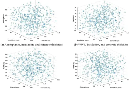
The Latin Hypercube Sampling Method (LHSM) [41] was used to generate the distribution of the simulation parameters used for constructing the sampling database. The LHSM generates a near-random sample of parameter values and ensures that the ensemble of random numbers is representative of the real variability. McKay [41] determined that a sample of 2×Nsampling data is enough (whereNis the number of variables). However, Conraud [42] and Magnier and Haghighat [20] found 22.5×Nsampling data is more appropriate to accurately sample the search space. In this study, a total of 450 cases were generated, which is slightly higher than the numbers recommended by Conraud [42] and Magnier and Haghighat [20]. Visualizations of selected design parameters from each of the four categories, x1for the thickness of concrete, x6for the insulation thickness, x11for the

absorption of solar radiation, and x16for the window-to-wall ratio (WWR), are presented in Figure3.

It can be observed that the 19-dimensional spaces are well covered with the 450 samples.

3. Prediction Model

3.1. Creation of the Sample Dataset

The Latin Hypercube Sampling Method (LHSM) [41] was used to generate the distribution of the simulation parameters used for constructing the sampling database. The LHSM generates a near-random sample of parameter values and ensures that the ensemble of random numbers is

representative of the real variability. McKay [41] determined that a sample of 2 × N sampling data is

enough (where N is the number of variables). However, Conraud [42] and Magnier and Haghighat

[20] found 22.5 × N sampling data is more appropriate to accurately sample the search space. In this

study, a total of 450 cases were generated, which is slightly higher than the numbers recommended by Conraud [42] and Magnier and Haghighat [20]. Visualizations of selected design parameters from

each of the four categories, x1 for the thickness of concrete, x6 for the insulation thickness, x11 for the

absorption of solar radiation, and x16 for the window-to-wall ratio (WWR), are presented in Figure 3.

It can be observed that the 19-dimensional spaces are well covered with the 450 samples.

(a)Absorptance, insulation, and concrete thickness (b) WWR, insulation, and concrete thickness

(c) WWR, absorptance, and concrete thickness (d) WWR, absorptance, and insulation thickness

Figure 3. Visualizations of selected design parameters.

All the simulation cases were run using DesignBuilder (DesignBuilder Software Ltd, Stroud, Gloucestershire, UK) with a time step of 30 min. It took around 45 days to create the 450 sample buildings and perform simulations using a desktop computer configured with an Intel i5 CPU @ 1.60 GHz with 4 GB of memory.

3.2. MLR Model

A multi-linear regression model is a very popular approach and was proved to be able to predict annual building energy consumption by Asadi et al. [43]. The regression model can be presented as:

f(x) = a + a x (6)

Figure 3.Visualizations of selected design parameters.

All the simulation cases were run using DesignBuilder (DesignBuilder Software Ltd, Stroud, Gloucestershire, UK) with a time step of 30 min. It took around 45 days to create the 450 sample buildings and perform simulations using a desktop computer configured with an Intel i5 CPU @ 1.60 GHz with 4 GB of memory.

3.2. MLR Model

(7)

f(x) =a0+ n

∑

i=1

aixi. (6)

where a0, a1, ..., and an are the estimations of the regression parameters, based on the

least-square method.

The regression model for the total building thermal load and discomfort degree hours can be presented as:

f1(x) =23029.4+158.9∗x1+242.6∗x2+701.5∗x3+238.8∗x24+1284.1∗x5−

9.6∗x6−10.99∗x7−15.62∗x8−11.15∗x9−16.12∗x10−2633.4∗x11−

2420.8∗x12−3749.1∗x13−3472.7∗x14−4228.5∗x15+101.4∗x16+62.21∗x17+

125.0∗x18+71.33∗x19.

(7)

f2(x) =3649.3−4.85∗x1+12.55∗x2+42.38∗x3+15.75∗x24+118.6∗x5−

0.5732∗x6−0.4843∗x7−0.9149∗x8−0.5462∗x9−0.7036∗x10−85.95∗x11−

112.9∗x12−203.2∗x13−139.7∗x14−172.9∗x15+11.06∗x16+7.377∗x17+

10.94∗x18+8.125∗x19.

(8)

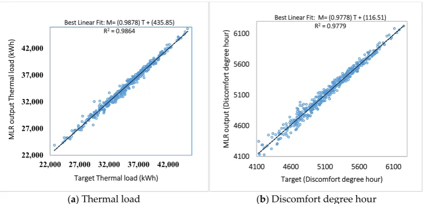
The regressions between the target simulated outputs and MLR predictions are presented in Figure4. Good agreements are found between the simulations and predictions, as the regression coefficients for both models are higher than 0.9889. A total of 405 (90%) sample data points were used for training and the remaining 45 (10%) sample data points were used for validation, which is the same as in Magnier and Haghighat [20]. For the thermal load model, the R2values for training and validation are 0.9840 and 0.9922, respectively. For the discomfort degree hour model, the R2_{values are}

0.9763 and 0.9860, respectively.

where a0, a1, ..., and an are the estimations of the regression parameters, based on the least-square

method.

The regression model for the total building thermal load and discomfort degree hours can be presented as:

f (x) = 23029.4 + 158.9 ∗ x + 242.6 ∗ x + 701.5 ∗ x + 238.8 ∗ x + 1284.1 ∗ x − 9.6 ∗ x − 10.99 ∗ x − 15.62 ∗ x − 11.15 ∗ x − 16.12 ∗ x − 2633.4 ∗ x −

2420.8 ∗ x − 3749.1 ∗ x − 3472.7 ∗ x − 4228.5 ∗ x + 101.4 ∗ x + 62.21 ∗ x + 125.0 ∗ x + 71.33 ∗ x

(7)

f (x) = 3649.3 − 4.85 ∗ x + 12.55 ∗ x + 42.38 ∗ x + 15.75 ∗ x + 118.6 ∗ x − 0.5732 ∗ x − 0.4843 ∗ x − 0.9149 ∗ x − 0.5462 ∗ x − 0.7036 ∗ x − 85.95 ∗ x − 112.9 ∗ x − 203.2 ∗ x − 139.7 ∗ x − 172.9 ∗ x + 11.06 ∗ x + 7.377 ∗ x + 10.94 ∗ x + 8.125 ∗ x

(8)

The regressions between the target simulated outputs and MLR predictions are presented in Figure 4. Good agreements are found between the simulations and predictions, as the regression coefficients for both models are higher than 0.9889. A total of 405 (90%) sample data points were used for training and the remaining 45 (10%) sample data points were used for validation, which is

the same as in Magnier and Haghighat [20]. For the thermal load model, the R2_{values for training}

and validation are 0.9840 and 0.9922, respectively. For the discomfort degree hour model, the R2

values are 0.9763 and 0.9860, respectively.

(a) Thermal load (b) Discomfort degree hour

Figure 4. Regression between MLR outputs and simulated targets.

3.3. ANN Model

ANN mimics the animal brain neural network behaviors in handling distributed parallel information. The ANN is interconnected with a number of joins (called neurons). Each join is connected with a number of inputs and outputs for information processing. The ANN learns the relationship between inputs and outputs through training data [44]. The ANN model was applied by Magnier and Haghighat [20] to predict the building thermal load and energy consumption with a maximum relative error of less than 10%.

A complete ANN model includes the inputs and corresponding weight values, thresholds, one or more hidden layers, and outputs. In this case, there are 19 inputs, one hidden layer, and one output layer. The number of nodes at the hidden layer is determined according to the following formulas [45]:

m < a − 1 (9)

Best Linear Fit: M= (0.9878) T + (435.85) R2_{= 0.9864}

22,000 27,000 32,000 37,000 42,000

22,000 27,000 32,000 37,000 42,000

MLR outp u t Therm al loa d (k W h )

Target Thermal load (kWh)

Best Linear Fit: M= (0.9778) T + (116.51) R2_{= 0.9779}

4100 4600 5100 5600 6100

MLR outp u t (Dis co m fo rt d egr ee hour )

Target (Discomfort degree hour)

Figure 4.Regression between MLR outputs and simulated targets.

3.3. ANN Model

(8)

A complete ANN model includes the inputs and corresponding weight values, thresholds, one or more hidden layers, and outputs. In this case, there are 19 inputs, one hidden layer, and one output layer. The number of nodes at the hidden layer is determined according to the following formulas [45]:

m<a−1. (9)

m<q(a+b) +c. (10)

m=log₂a (11)

where m is the number of nodes at the hidden layer; a is the number of nodes at the input layer (equal to 19 in this study); b is the number of output nodes; and c is a constant, which is between 0 and 10. The optimal number of nodes in the hidden layer in this study is 8.

Figure5presents the diagram of the ANN model in this study. The maximum number of epochs is 200. The learning speed is 0.03, and the target error precision is 5×10−5. The number of sample data for training and for validation are 405 (90%) and 45 (10%), respectively.

m < (a + b) + c (10)

m = log a (11)

Figure 5 presents the diagram of the ANN model in this study. The maximum number of epochs is 200. The learning speed is 0.03, and the target error precision is 5 × 10−5_{. The number of} sample data for training and for validation are 405 (90%) and 45 (10%), respectively.

Figure 5. ANN model diagram.

The regressions between the target simulated outputs and MLR predictions are presented in Figure 6. Good agreements are found between the simulations and predictions with regression coefficients for both models close to 1.0. For the thermal load model, the R2_{values for training and} validation are 0.9901 and 0.9962, respectively. For the discomfort degree hour model, the R2_values are 0.9892 and 0.9966, respectively.

Figure 6. Regression between ANN outputs and simulated targets.

3.4. Comparisons on Different Prediction Models

The comparisons on the performance of the two prediction models are presented in Table 4. It can be found that both the regression coefficients are higher than 0.989, which indicates very good agreements between the simulation and prediction outcomes. The ANN models perform better with higher regression coefficients and lower standard deviations. It can also be found that the relative

Best Linear Fit: A = (0.98) T + (671.24) R2_{= 0.9924}

22,000 27,000 32,000 37,000 42,000

ANN o utpu t Ther m al lo ad ( kW h )

4100 4600 5100 5600 6100

4100 5100 6100

A N Noutput (D iscomfor t d eg ree h o u r)

Target (Discomfort degree hour) Figure 5.ANN model diagram.

The regressions between the target simulated outputs and MLR predictions are presented in Figure6. Good agreements are found between the simulations and predictions with regression coefficients for both models close to 1.0. For the thermal load model, the R2_{values for training and}

validation are 0.9901 and 0.9962, respectively. For the discomfort degree hour model, the R2values are 0.9892 and 0.9966, respectively.

m < (a + b) + c (10)

m = log a (11)

Figure 5 presents the diagram of the ANN model in this study. The maximum number of

epochs is 200. The learning speed is 0.03, and the target error precision is 5 × 10−5_{. The number of}

sample data for training and for validation are 405 (90%) and 45 (10%), respectively.

Figure 5. ANN model diagram.

The regressions between the target simulated outputs and MLR predictions are presented in Figure 6. Good agreements are found between the simulations and predictions with regression

coefficients for both models close to 1.0. For the thermal load model, the R2_{values for training and}

validation are 0.9901 and 0.9962, respectively. For the discomfort degree hour model, the R2_values

are 0.9892 and 0.9966, respectively.

Figure 6. Regression between ANN outputs and simulated targets.

3.4. Comparisons on Different Prediction Models

The comparisons on the performance of the two prediction models are presented in Table 4. It can be found that both the regression coefficients are higher than 0.989, which indicates very good agreements between the simulation and prediction outcomes. The ANN models perform better with higher regression coefficients and lower standard deviations. It can also be found that the relative

22,000 27,000 32,000 37,000 42,000

ANN o utpu t Ther m al lo ad ( kW h )

4100 4600 5100 5600 6100

4100 5100 6100

A N Noutput (D iscomfor t d eg ree h o u r)

Target (Discomfort degree hour)

(9)

3.4. Comparisons on Different Prediction Models

The comparisons on the performance of the two prediction models are presented in Table4. It can be found that both the regression coefficients are higher than 0.989, which indicates very good agreements between the simulation and prediction outcomes. The ANN models perform better with higher regression coefficients and lower standard deviations. It can also be found that the relative errors of the discomfort degree hour models are always lower than the thermal load models. The maximum errors for all the models are less than 8%.

Table 4.Comparison on the performance of the four prediction models.

Method

Thermal Load Discomfort Degree Hour

Regression Coefficient

Standard Deviation (kWh)

Maximum Relative Error/Maximum Absolute Error (kWh)

Regression Coefficient

Standard Deviation (◦C·h)

Maximum Relative Error/Maximum Absolute Error (◦C·h)

MLR 0.992 514.183 7.01%/1930.72 0.989 61.689 6.91%/354.32

ANN 0.996 362.28 6.01%/1380.70 0.996 36.235 3.51%/145.05

4. Results and Discussion

Since the prediction results from all models are in good agreement with simulation results, the ANN models and MLR models are coupled with a multi-objective genetic algorithm to find the optimal design solutions.

4.1. MLR with GA

The regression models (Equations (7) and (8)) are used as the fitness functions for a multi-objective optimization program using genetic algorithm developed in MATLAB. The constraints of the variables are presented as follows:

0.05≤x1, x2, x3, x4, x5≤0.25 (12)

10≤x6, x7, x8, x9, x10 ≤100 (13)

0.1≤x11, x12, x13, x14, x15 ≤0.9 (14)

10≤x16, x17, x18, x19 ≤80 (15)

The program ran a number of times and each time came out with 1–4 Pareto front solutions when converged. A total of 45 solutions are obtained after 29 runs, after which the ranges of the outcomes for each design parameter stays unchanged. The maximum, minimum, median, average values, and standard deviations for the outcomes of the thermal load, number of discomfort degree hours, and each variable are summarized in Table5.

Table 5.Statistical values of the objective functions and design variables for MLRGA.

Item Minimum Maximum Median Average Standard Deviation

Thermal load (kWh) 19,568.9 20,868.4 20,127.2 20,162.6 333.3

Ndis(◦C·h) 3721.2 3822.1 3767.4 3766.7 23.8

x1(m) 0.1553 0.2500 0.2466 0.2369 0.0221

x2(m) 0.1564 0.2500 0.2428 0.2351 0.0230

x3(m) 0.1947 0.2500 0.2498 0.2436 0.0111

x4(m) 0.1775 0.2500 0.2493 0.2425 0.0155

x5(m) 0.1751 0.2500 0.2500 0.2455 0.0126

x6(mm) 31.5311 84.9766 52.9107 54.2241 13.5953

x7(mm) 31.8788 74.5924 54.3463 54.5520 10.9994

x8(mm) 42.5186 78.8962 63.8735 62.7198 9.6804

x9(mm) 36.1280 79.5128 63.2697 58.2602 11.8191

(10)

Table 5.Cont.

x11 0.1881 0.8366 0.4236 0.4398 0.1299

x12 0.2061 0.6710 0.3713 0.4325 0.1551

x13 0.1105 0.5694 0.2520 0.2656 0.0892

x14 0.1643 0.7348 0.3544 0.3960 0.1348

x15 0.1059 0.4254 0.1665 0.1865 0.0856

x16(%) 10.4783 14.4398 11.2875 11.4404 0.8348

x17(%) 10.5023 15.7129 12.1651 12.4202 1.4820

x18(%) 10.3139 12.8394 11.1387 11.2782 0.6253

x19(%) 10.5941 14.3469 11.7449 11.9172 0.8638

It is observed that the medians for the thickness of the concrete layer are higher than 0.24 m; for the insulation layer, are 52.9–63.9 mm; for the absorptance of solar radiation, are 0.167–0.424; and for the window-to-wall ratio, are 11.1–12.2%. There are differences on the values of design variables at different orientations, meaning the building can be adaptively designed to minimize the impact of outside weather conditions on the indoor environment.

The thermal load and number of discomfort degree hours for the best solution are 19,568.9 kWh and 3721.2◦C·h (19,000.4 kWh and 3755.4◦C·h from DesignBuilder (DesignBuilder Software Ltd., Stroud, Gloucestershire, UK)), while the ones for the base building are 23,233.0 kWh and 4840.0◦C·h. The reduction on the thermal load and number of discomfort degree hours are 18.2% and 22.4%, respectively. The relative errors on the predictions of the thermal load and discomfort degree hours are 2.99% and−0.91%, respectively.

4.2. ANN with GA

The ANN models developed in Section3.3are used as the fitness functions for the multi-objective optimization program, and the same constraints of the variables as in Section4.1are applied.

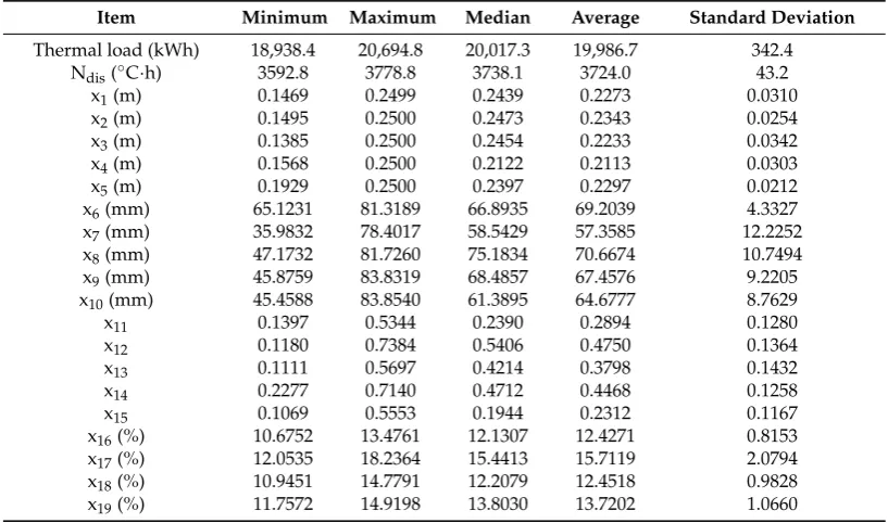
The program ran for a number of times and each time came out with 1–12 Pareto front solutions. A total of 44 solutions are obtained after 14 runs. The maximum, minimum, median, average values, and standard deviation for the outcomes of the thermal load, number of discomfort hours, and each variable are summarized in Table6.

Table 6.Statistical values of the objective functions and design variables for ANNGA.

Thermal load (kWh) 18,938.4 20,694.8 20,017.3 19,986.7 342.4

Ndis(◦C·h) 3592.8 3778.8 3738.1 3724.0 43.2

x1(m) 0.1469 0.2499 0.2439 0.2273 0.0310

x2(m) 0.1495 0.2500 0.2473 0.2343 0.0254

x3(m) 0.1385 0.2500 0.2454 0.2233 0.0342

x4(m) 0.1568 0.2500 0.2122 0.2113 0.0303

x5(m) 0.1929 0.2500 0.2397 0.2297 0.0212

x6(mm) 65.1231 81.3189 66.8935 69.2039 4.3327

x7(mm) 35.9832 78.4017 58.5429 57.3585 12.2252

x8(mm) 47.1732 81.7260 75.1834 70.6674 10.7494

x9(mm) 45.8759 83.8319 68.4857 67.4576 9.2205

x10(mm) 45.4588 83.8540 61.3895 64.6777 8.7629

x11 0.1397 0.5344 0.2390 0.2894 0.1280

x12 0.1180 0.7384 0.5406 0.4750 0.1364

x13 0.1111 0.5697 0.4214 0.3798 0.1432

x14 0.2277 0.7140 0.4712 0.4468 0.1258

x15 0.1069 0.5553 0.1944 0.2312 0.1167

x16(%) 10.6752 13.4761 12.1307 12.4271 0.8153

x17(%) 12.0535 18.2364 15.4413 15.7119 2.0794

x18(%) 10.9451 14.7791 12.2079 12.4518 0.9828

(11)

It is observed that the medians for the thickness of the concrete layer are higher than 0.21 m, for the insulation layer are 58.5–75.2 mm, for the absorbance of solar radiation are 0.194–0.5406, and for the window-to-wall ratio are 12.1–15.4%.

The thermal load and number of discomfort degree hours for the best solution are 18,938.4kWh and 3592.8◦C·h (19,276.63 kWh and 3773.5◦_{C·h from DesignBuilder (DesignBuilder Software Ltd.,}

Stroud, Gloucestershire, UK)). The reduction on the thermal load and number of discomfort degree hours are 17.0% and 22.2%, respectively. The relative errors on the predictions of the thermal load and discomfort degree hours are 1.75% and 4.76%, respectively.

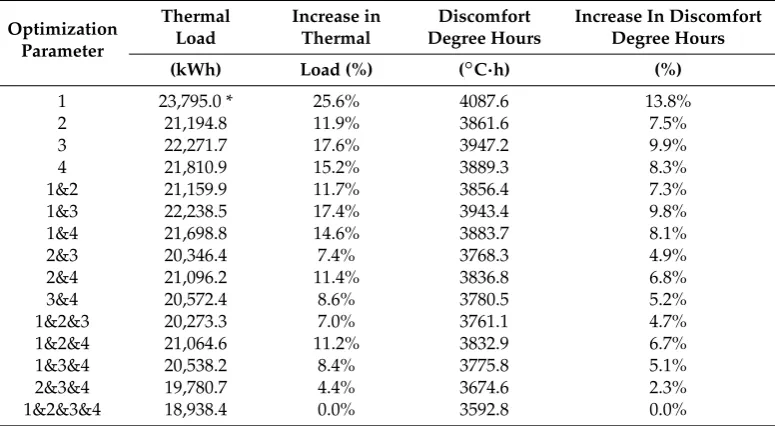
4.3. Optimization with Different Combinations of Parameters

The ANNGA approach is applied for optimization on different combinations of parameters. The results on the optimization are presented in Table7, where “1” refers to the concrete thickness; “2” refers to the insulation thickness; “3” refers to the absorptance of solar radiation; and “4” refers to the window-to-wall ratio. The results clearly show that when one more group of parameters is added, there is a further improvement on the building performance.

Table 7.Comparison on the optimal solutions using different combinations of design parameters.

Optimization Parameter

Thermal Load

Increase in Thermal

Discomfort Degree Hours

Increase In Discomfort Degree Hours

(kWh) Load (%) (◦C·h) (%)

1 23,795.0 * 25.6% 4087.6 13.8%

2 21,194.8 11.9% 3861.6 7.5%

3 22,271.7 17.6% 3947.2 9.9%

4 21,810.9 15.2% 3889.3 8.3%

1&2 21,159.9 11.7% 3856.4 7.3%

1&3 22,238.5 17.4% 3943.4 9.8%

1&4 21,698.8 14.6% 3883.7 8.1%

2&3 20,346.4 7.4% 3768.3 4.9%

2&4 21,096.2 11.4% 3836.8 6.8%

3&4 20,572.4 8.6% 3780.5 5.2%

1&2&3 20,273.3 7.0% 3761.1 4.7%

1&2&4 21,064.6 11.2% 3832.9 6.7%

1&3&4 20,538.2 8.4% 3775.8 5.1%

2&3&4 19,780.7 4.4% 3674.6 2.3%

1&2&3&4 18,938.4 0.0% 3592.8 0.0%

* The prediction on the thermal load of the base case building is 24,000.9 kWh. Through optimization, only 46.8% of concrete for the east wall is needed as compared to the base building. It is found that when the insulation thickness is higher than 60 mm, the reduction on thermal load and discomfort degree hours by increasing the insulation thickness is very small (less than a 2% reduction on thermal load per 10 mm increase in insulation thickness and no reduction when insulation thickness increases to 200 mm). The thickness of insulation needs to be at least 200 mm (about four times the thickness of the optimal solution) to reduce the same thermal load as the optimal solution. However, the discomfort degree hour stays at 3831.3◦C·h. The thermal load and discomfort degree hours do not decrease with further increase in the insulation thickness. The cost of changing all this variables to get the optimized solution is ¥23,686.911 less than by simply increasing the thickness of insulation to 200 mm. In addition, the increase of wall thickness will lead to less internal space for same floor area, which is not a preferred option.

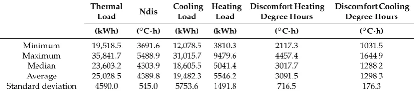
4.4. Optimization with Four Objective Functions

The ANN models for the total hourly cooling load (QC), heating load (QH), discomfort heating

degree hours (IW), and cooling degree hours (IS) are developed and used as fitness functions for

(12)

Table 8.Pareto front solutions characteristic for four objective functions.

Thermal

Load Ndis

Cooling Load

Heating Load

Discomfort Heating Degree Hours

Discomfort Cooling Degree Hours

(kWh) (◦C·h) (kWh) (kWh) (◦C·h) (◦C·h)

Minimum 19,518.5 3691.6 12,078.5 3810.3 2117.3 1031.5

Maximum 35,841.7 5488.9 31,015.7 9479.6 4457.4 1644.9

Median 23,603.2 4303.9 18,605.5 5041.4 3017.7 1288.2

Average 25,028.5 4389.8 19,482.3 5546.2 3091.5 1298.3

Standard deviation 4590.0 545.0 5753.6 1491.8 716.5 176.3

Notes: minimum cooling load, and minimum heating load might not happen at the same time; similarly, minimum discomfort heating degree hours and minimum discomfort cooling degree hours might not occur at the same time.

It can be found that although a few solutions can achieve total thermal load and number of discomfort degree hours as low as the ones presented in Sections4.1and4.2, the average values of which are much higher, indicating lower optimization performance. Therefore, two objective functions are sufficient for optimization purpose.

5. Conclusions

In this paper, an MLR model and ANN model are developed to predict the building thermal load and the number of discomfort degree hours considering the variable thermal mass, insulation, absorptance of solar radiation, and glazing ratio. The MLR models and ANN models are coupled with a multi-objective genetic optimization algorithm to minimize the building thermal load and improve the thermal comfort for a very energy-efficient two-star green building in China. Finally, optimization with four objective functions is also performed. The following conclusions can be made:

(1) The ANN models perform better than the MLR models in terms of regression coefficients, standard deviations, and absolute errors. The relative errors of the discomfort degree hour models are always lower than the thermal load models.

(2) When used as fitness functions for GA to obtain the optimal building design solutions, the MLR model and ANN model have similar performances.

(3) The optimal solutions prefer concrete layer with median thickness higher than 0.21 m; insulation layer, 52.9–75.2 mm; absorbance of solar radiation, 0.167–0.5406; and window-to-wall ratio, 11.1–15.4%.

(4) The optimal design solutions help to reduce the thermal load and the number of discomfort hours of the two-star green building by up to 18.2% and 22.4%, respectively.

(5) The two objective functions are better than the four objective functions to perform the optimization on thermal load and thermal comfort.

Acknowledgments: Natural Science Foundation of Hubei Province under grant (2017CFB602) and Hunan Provincial Department of housing and urban rural development under grant (KY2016063).

Author Contributions:Yaolin Lin and Wei Yang contributed to the conception of the study and the development of the methodology. Yaolin Lin and Shiquan Zhou developed the computer models, and simulated and analyzed the data. Yaolin Lin, Wei Yang, and Chun-Qing Li wrote the manuscript. All the authors have read and approved the final manuscript.

(13)

Abbreviations

ANN Artificial neural network

CDD Cooling degree day

GA Genetic algorithm

HDD Heating degree day

MLR Multi-linear regression OAT Outdoor air temperature

a Number of nodes at the input layer ai Coefficient for the regression model

b Number of output nodes

c Constant, between 0 and 10

f1 Total building thermal load, kWh

f2 Total number of discomfort degree hours,◦C·h IS Cooling discomfort degree hours,◦C·h IW Heating discomfort degree hours,◦C·h m Number of nodes at the hidden layer

n Number of the design variables, equal to 19 in this study QC Total hourly cooling load, kWh

QH Total hourly heating load, kWh

tH Higher limit temperature in the thermal comfort range,◦C ti Indoor air temperature at time i,◦C

tL Lower limit temperature in the thermal comfort range,◦C x Combination of the design-variables (x1, x2, ..., xn)

References

1. IEA. 2015. Buildings Energy Use in China, Transforming Construction and Influencing Consumption to 2050. Available online:http://www.iea.org(assessed on 5 October 2017).

2. EAI. 2017. How Much Energy Is Consumed in U.S. Residential and Commercial Buildings? Available online:

https://www.eia.gov/tools/faqs/faq.php?id=86&t=1(assessed on 5 October 2017).

3. Filippin, C.; Larsen, S.F.; Beascochea, A.; Lesino, G. Response of conventional and energy-saving buildings to design and human dependent factors.Sol. Energy2005,78, 455–470. [CrossRef]

4. Badescu, V.; Laaser, N.; Crutescu, R.; Crutescu, M.; Dobrovicescu, A.; Tsatsaronis, G. Modeling, validation and time-dependent simulation of the first large passive building in Romania.Renew. Energy2011,36, 142–157. [CrossRef]

5. Gong, X.; Akashi, Y.; Sumiyoshi, D. Optimization of passive design measures for residential buildings in different Chinese areas.Build. Environ.2012,58, 46–57. [CrossRef]

6. Zhu, Y.Built Environment, 4th ed.; China Architectural Engineering Industrial Publishing Press: Beijing, China, 2016.

7. Delgarm, N.; Sajadi, B.; Delgarm, S. Multi-objective optimization of building energy performance and indoor thermal comfort: A new method using artificial bee colony (ABC).Energy Build.2016,131, 42–53. [CrossRef] 8. Ascione, F.; Bianco, N.; De Stasio, C.; Mauro, G.M.; Vanoli, G.P. A new comprehensive approach for cost-optimal building design integrated with the multi-objective model predictive control of HVAC systems.

Sustain. Cities Soc.2017,31, 136–150. [CrossRef]

9. Brea, F.; Fachinotti, V.D. A computational multi-objective optimization method to improve energy efficiency and thermal comfort in dwelling.Energy Build.2017,154, 283–294. [CrossRef]

10. Brea, F.; Silva, A.S.; Ghisi, E.; Fachinotti, V.D. Residential building design optimisation using sensitivity analysis and genetic algorithm.Energy Build.2016,133, 853–866. [CrossRef]

11. Ascione, F.; Bianco, N.; De Stasio, C.; Mauro, G.M.; Vanoli, G.P. A new methodology for cost-optimal analysis by means of the multi-objective optimization of building energy performance.Energy Build.2015,88, 78–90. [CrossRef]

12. Ihm, P.; Krarti, M. Design optimization of energy efficient residential buildings in Tunisia.Build. Environ.

(14)

13. Evins, R. Multi-level optimization of building design, energy system sizing and operation. Energy2015,

90, 1775–1789. [CrossRef]

14. Krarti, M.; Deneuville, A. Comparative evaluation of optimal energy efficiency designs for French and US office buildings.Energy Build.2015,93, 332–344. [CrossRef]

15. Xu, J.; Kim, J.; Hong, H.; Koo, J. A systematic approach for energy efficient building design factors optimization.Energy Build.2015,89, 87–96. [CrossRef]

16. Delgarm, N.; Sajadi, B.; Delgarm, S.; Kowsary, F. A novel approach for the simulation-based optimization of the buildings energy consumption using NSGA-II: Case study in Iran.Energy Build.2016,127, 552–560. [CrossRef]

17. Yong, S.; Kim, J.; Gim, Y.; Kim, J.; Cho, J.; Hong, H.; Baik, Y.; Koo, J. Impacts of building envelope design factors upon energy loads and their optimization in US standard climate zones using experimental design.

Energy Build.2017,141, 1–15. [CrossRef]

18. Caldas, L.G.; Norford, L.K. A design optimization tool based on a genetic algorithm.Automat. Constr.2002,

11, 173–184. [CrossRef]

19. Wang, W.; Zmeureanu, R.; Rivard, H. Applying multi-objective genetic algorithms in green building design optimization.Build. Environ.2005,40, 1512–1525. [CrossRef]

20. Magnier, L.; Haghighat, F. Multiobjective optimization of building design using TRNSYS simulations, genetic algorithm, and Artificial Neural Network.Build. Environ.2010,45, 739–746. [CrossRef]

21. Bichiou, Y.; Krarti, M. Optimization of envelope and HVAC systems selection for residential buildings.

Energy Build.2011,43, 3373–3382. [CrossRef]

22. Ramallo-González, A.P.; Coley, D.A. Using self-adaptive optimisation methods to perform sequential optimisation for low-energy building design.Energy Build.2014,81, 18–29. [CrossRef]

23. Yu, W.; Li, B.; Ji, H.; Zhang, M.; Wang, D. Application of multi-objective genetic algorithm to optimize energy efficiency and thermal comfort in building design.Energy Build.2015,88, 135–143. [CrossRef]

24. Liu, S.; Meng, X.; Tam, C. Building information modeling based building design optimization for sustainability.Energy Build.2015,105, 139–153. [CrossRef]

25. Lin, Y.; Tsai, K.; Lin, M.; Yang, M. Design optimization of office building envelope configurations for energy conservation.Appl. Energy2016,171, 336–346. [CrossRef]

26. Azari, R.; Garshasbi, S.; Amini, P.; Rashed-Ali, H.; Mohammadi, Y. Multi-objective optimization of building envelope design for life cycle environmental performance.Energy Build.2016,126, 524–534. [CrossRef] 27. Zhang, A.; Bokel, R.; Dobbelsteen, A.V.D.; Sun, Y.; Huang, Q.; Zhang, Q. Optimization of thermal and

daylight performance of school buildings based on a multi-objective genetic algorithm in the cold climate of China.Energy Build.2017,139, 371–384. [CrossRef]

28. Bambrook, S.M.; Sproul, A.B.; Jaco, D. Design optimisation for a low energy home in Sydney.Energy Build.

2011,43, 1702–1711. [CrossRef]

29. Baglivo, C.; Congedo, P.M.; Fazio, A. Multi-criteria optimization analysis of external walls according to ITACA protocol for zero energy buildings in the mediterranean climate.Build. Environ.2014,82, 467–480. [CrossRef]

30. Hamdy, M.; Hasan, A.; Siren, K. Applying a multi-objective optimization approach for Design of low-emission cost-effective dwellings.Build. Environ.2011,46, 109–123. [CrossRef]

31. Romani, Z.; Draoui, A.; Allard, F. Metamodeling the heating and cooling energy needs and simultaneous building envelope optimization for low energy building design in Morocco.Energy Build.2015,102, 139–148. [CrossRef]

32. Carreras, J.; Boer, D.; Cabeza, L.F.; Jiménezc, L.; Guillén-Gosálbez, G. Eco-costs evaluation for the optimal design of buildings with lower environmental impact.Energy Build.2016,119, 189–199. [CrossRef] 33. Pal, S.K.; Takano, A.; Alanne, K.; Siren, K. A life cycle approach to optimizing carbon footprint and costs of a

residential building.Build. Environ.2017,123, 146–162. [CrossRef]

34. Shi, X. Design optimization of insulation usage and space conditioning load using energy simulation and genetic algorithm.Energy2011,36, 1659–1667. [CrossRef]

35. Yang, C.; Li, H.; Rezgui, Y.; Petri, I.; Yuce, B.; Chen, B.; Jayan, B. High throughput computing based distributed genetic algorithm for building energy consumption optimization.Energy Build.2014,76, 92–101. [CrossRef]

(15)

37. Gossard, D.; Lartigue, B.; Thellier, F. Multi-objective optimization of a building envelope for thermal performance using genetic algorithms and artificial neural network. Energy Build. 2013, 67, 253–260. [CrossRef]

38. Zhang, Y.; Lin, K.; Zhang, Q.; Di, H. Ideal thermophysical properties for free-cooling (or heating) buildings with constant thermal physical property material.Energy Build.2006,38, 1164–1170. [CrossRef]

39. Ministry of Housing and Urban-Rural Development of the People’s Republic of China (MOHURD) JGJ134-2010.Residential Building Energy Efficiency Design Standard for Hot Summer/Cold Winter Region; China Architectural Engineering Industrial Publishing Press: Beijing, China, 2010.

40. GB-T50378 2014. Ministry of Housing and Urban-Rural Construction of the People’s Republic of China.

Assessment Standard for Green Building; China Architectural Engineering Industrial Publishing Press: Beijing, China, 2014.

41. McKay, M.D.Sensitivity Arid Uncertainty Analysis Using a Statistical Sample of Input Values, Uncertainty Analysis; CRC Press: Boca Raton, FL, USA, 1988; pp. 145–186.

42. Conraud, J. A Methodology for the Optimization of Building Energy, Thermal, and Visual Performance. Master’s Thesis, Concordia University, Montreal, QC, Canada, 2008.

43. Asadi, S.; Amiri, S.S.; Mottahedi, M. On the development of multi-linear regression analysis to assess energy consumption in the early stages of building design.Energy Build.2014,85, 246–255. [CrossRef]

44. Kalogirou, S.A. Applications of artificial neural networks in energy systems.Energy Convers. Manag.1999,

40, 1073–1087. [CrossRef]

45. Wang, X.; Shi, F.; Yu, L.; Li, Y.Analysis on 43 Neural Network Application Cases Using MATLAB; Beijing University of Aeronautics and Astronautics Publishing Press: Beijing, China, 2013.