Automated scheduling of Household Appliances
using Predictive Mixed Integer Programming
Himanshu Nagpal1,* , Andrea Staino1,2and Biswajit Basu1
1 Department of Civil, Structural and Environmental Engineering, Trinity College Dublin, Dublin 2, Ireland; [email protected]
2 PHM Center of Excellence, ALSTOM, Saint-Ouen, France; [email protected]
* Correspondence: [email protected]; Tel.: +353-892161483
Abstract: In this work, an algorithm for the scheduling of household appliances to reduce the energy cost and the peak-power consumption is proposed. The system architecture of a home energy management system (HEMS) is presented to operate the appliances. The dynamics of thermal and non-thermal appliances is represented into state-space model to formulate the scheduling task into a mixed-integer-linear-programming (MILP) optimization problem. Model predictive control (MPC) strategy is used to operate the appliances in real-time. The HEMS schedules the appliances in dynamic manner without any a priori knowledge of the load-consumption pattern. At the same time, HEMS responds to the real-time electricity market and the external environmental conditions (solar radiation, ambient temperature etc). Simulation results exhibit the benefits of proposed HEMS by showing the reduction of upto 47% in electricity cost and upto 48% in peak power consumption.
Keywords:Home energy management system, Flexible demand-response, optimal load-scheduling, Mixed Integer Programming, Predictive control, demand-side-management
Nomenclature
(U A)t Thermal conductance of the water tank
(U A)f r heat transfer coefficient between floor and room air (U A)ra heat transfer coefficient between room air and ambient
(U A)w f heat transfer coefficient between water and floor
η efficiency of heat pump
ηh efficiency of heating element in the water tank
A set of appliances
P set of thermal appliances Q set of non-thermal appliances
Ωj total running time ofjthnon-thermal appliance to complete the task
φs solar radiation power
Ct specific heat capacity of the water tank
Cp,f heat capacity of floor
Cp,r heat capacity of room air
Cp,w heat capacity of water
p fraction of incident solar radiation on floor
Ph controlled power consumption by heating element in the water tank
Qc energy consumed from the water tank
Ta ambient temperature
Tf floor temperature
Ti inlet water temperature
Tr room air temperature
Tt water tank temperature
Tw water temperature
Wc work done by the compressor
1. Introduction
Building energy consumption contributes approximately 20% to 40% to the total energy consumption in developed countries and has exceeded other major sectors like industrial and transportation [1]. Smart grid is a major step forward to an energy efficient future of the humankind which allows integration of advanced sensing and communication technologies and various control methodologies in order to achieve optimum energy flow [2]. One of the important features of smart grid is the development and incorporation of demand-response strategies [3].
Demand-response [4], [5] refers to “the change in electric usage by end-use customer from their normal consumption patterns in response to change in price of electricity over time, or incentive payments designed to induce lower electricity use at times of high wholesale market prices or when system reliability is jeopardized” [6]. In simple words, it is the change in power consumption by the customer to better match the load-demand with the power supply. The customer may adjust the load-demand by postponing some tasks that require larger amount of electric power or may decide to pay higher prices for the electricity in order to complete the tasks. Obviously, it is difficult for the consumer to manually participate in demand-response programs. This explicates the need of an automated system to communicate with smart grid and make optimal decisions on behalf of the customer to achieve the goal of demand-response strategy.
This automated system usually called home energy management system (HEMS) is connected to smart-grid by means of bi-directional communications. Advanced sensors and smart-meters are employed to receive/send data and control signals between smart-home and the power utility [7]. Advanced control algorithms are incorporated into HEMS to schedule or operate the appliances in the desired way. The development of appropriate scheduling algorithms has been isolated as one of the crucial challenges for the next generation of real-time systems [8]. Extensive research has been dedicated to the problem of electric load scheduling with focus on different objectives such as customer comfort [9], minimization of electricity cost [10], reduction of energy usage [11] and shifting the electric load [12] etc. Moreover, various methods have been used to investigate this problem which include, mixed-integer programming [13–15], stochastic programming [16,17], evolutionary algorithms [18,19], heuristic-based algorithms [20? ?,21] and learning-based algorithms [22,23].
The above mentioned studies do not consider the dynamic characteristic of the appliance scheduling. In other words, the optimization problem is solved once for the whole day rather than updating at each time step, which may not be optimal since the load-demand may not be same for each day. The immediate load-demand can not be met with the above approaches. In these cases, prior information (either expected or real) about the load-demand needs to be available. The MPC (receding horizon control) is the solution to this issue. MPC is an advanced method of control that emerges from application in process industry in late 70s and early 80s [29]. MPC represents a class of advanced control methods in which the model of the process is considered explicitly to predict the future evolution of the process to optimize the control input while respecting certain constraints. So, in this case, the optimization problem is solved at each time step with updated values of the load-demand, electricity prices and other relevant information like external weather conditions. A few studies have investigated the use of MPC strategy for appliance-scheduling. The authors in [30] investigated the problem of load-scheduling of thermal and non-thermal appliances using MPC under different price schemes and achieves the total electricity cost saving of up to 20%. But the previous study do not focus on the peak-load reduction by employing constraints on the total maximum power consumption. In [31], the author addressed the similar problem of deferrable appliance-scheduling considering distributed generation (DG) using a multi-time stochastic MPC to consider the uncertainty emerged due to the intermittent DG power. In the best case scenario, the total electricity cost reduction of 53% is achieved in this study. The limitation of the previous study is that some deferrable appliances are operated during a fixed optimal time interval only which is obtained using genetic algorithm. This takes away the flexibility for the customer to intervene for using the appliances at desired time intervals.
2. Research Contribution
After identifying the gap in the literature, in the present study, an architecture of HEMS is presented for automated scheduling of appliances with an objective of reducing the peak-power consumption and the total electricity cost. It is assumed that the bi-directional communication between the house and the power grid is present, which enables the HEMS to receive/ send data and control signal from the power utility. HEMS is employed in real-time electricity pricing environment and is designed to operate in two modes of operation (MOO) based upon the load category (thermal/ non-thermal).
The optimization problem is formulated and solved at each time step using receding horizon framework. In the Mode 2, only the thermal-appliances are activated. The optimization problem is formulated into a linear-program (LP) with constraints and the objective of reducing the energy cost. At each time step, updated system state and predicted information by the forecaster becomes available which is used by the HEMS. The Mode 1 is switched on when the customer requests to run a non-thermal appliance. In the Mode 1, a predictive MILP is formulated with the same objective. However, additional constraints are introduced to ensure that the task assigned to the non-thermal appliance is finished by the specified deadline. In both the modes, soft constraints on the maximum power consumption of the appliances is also imposed. This way, the total peak power consumption is maintained under the specified peak-consumption capacity. The constraint values are decided by the utility company or the aggregator based upon the demand of electricity and operational cost of the grid. These values are communicated to the smart-meter in homes for a fixed duration in advance and updated at each time step.
3. Load Categorization
Before going into a detailed description and working methodology of the HEMS, the classification of electrical load is detailed in this section. The load is classified based upon the dynamics of the appliances. The classification is important for the HEMS, based upon this classification it makes the choice that in which MOO it should run. So, the overall electrical load is divided into two categories.
3.1. Thermal load
This category includes the electrical load consumed by the appliances which are thermal in nature i.e. their system dynamics include temperature as a system-state.e.g.heat pump, room heater, water heater, refrigerator etc.
3.2. Non-thermal load
In this category, electrical load consumed by the appliances which are non-thermal in nature is included. These non-thermal appliances are assumed to have following characteristics.
• Preemptive - The appliance can be paused or interrupted whenever needed.
• Fixed duration - The appliance run for a fixed duration (Ω) to finish the task assigned to it. • Deadline - The appliance has a deadline associated by which it needs to finish the task assigned
to the appliance. The deadline is chosen by the user and cannot be smaller than the running duration of the appliance which is an operational constraint [30]. Examples include washing machine, clothes dryer, dishwasher etc.
4. System Architecture
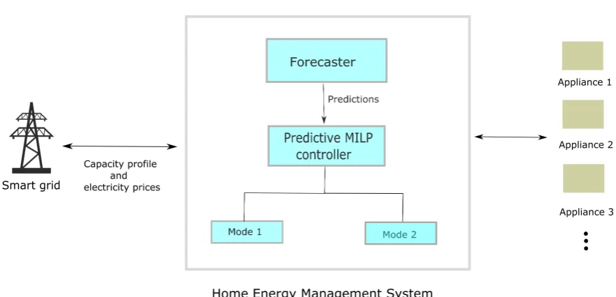
This section provides a detailed description of the HEMS. The system architecture of the HEMS is presented in the Figure1. The main components of the HEMS are described below.
• The first component of the HEMS is the forecaster. It is deputized to make predictions about the external weather and the heat-gains due to solar irradiance in the house. Data-driven prediction techniques [32], [33] are commonly used to make these predictions based on available historical data about the variable. The second component of the HEMS uses these predictions to optimally schedule the thermal appliances.
• The second and the key component of the HEMS is the Predictive MILP controller. This component operates in two MOO, which is determined automatically within the component based upon the electrical load categories (see section3). In each mode, a different mathematical optimization problem is solved by exploiting the predictions made by the forecaster about the weather conditions. The electricity prices and the consumption-capacity profile is provided to HEMS by the smart-grid operator using smart-meter communication.
5. Appliance Dynamics Modelling and Setup
5.1. State-space model
In order to apply the proposed scheduling algorithm, the dynamics of all the appliances are modelled mathematically into a discrete linear time-invariant state-space representation. The discrete state-space model of a linear system with control inputs (m), outputs (p), state variables (n) and external disturbances (r) is written as following in equation1[34]
xk+1= Axk+Buk+Edk
yk=Cxk
Figure 1.System architecture of HEMS
x ∈ Rnis thestate vector,u ∈
Rm is thecontrol vector,y ∈ Rpis called theoutput vectorandd ∈ Rr
is called thedisturbance vector. Similarly,A∈ Rn×nis thestate matrix,B∈
Rn×mis thecontrol matrix,
C∈Rp×nis theoutput matrixandE∈Rr×nis thedisturbance matrix.kdenotes the time instant.
5.2. Thermal load appliances modelling
For purpose of heating the indoor environment, the house is considered to be equipped with a ground-source heat pump through floor heating pipes [35]. For hot water requirements, building is connected to a solar water heater system. The dynamics of both the systems is influenced by the solar irradiance and the ambient temperature.
5.2.1. Heat pump
A reduced order model of a residential building equipped with a ground source heat-pump is developed in [35] and [36] as follows
Cp,rT˙r = (U A)f r(Tf−Tr)−(U A)ra(Tr−Ta) + (1−p)φs
Cp,fT˙f = (U A)w f(Tw−Tf)−(U A)f r(Tf −Tr) +pφs
Cp,wT˙w =ηWc−(U A)w f(TW−Tf)
(2)
The system of equations (2) is discretized with appropriate sample time using zero-order-hold model and written into state-space representation as in equation (1). Subsequently for heat pump state-space model, we getx=hTr Tf Tw
iT
,u=Wc,d=
h Ta φs
iT
andy=Tr.
5.2.2. Solar water tank
The heat dynamics of the solar water tank is described using simple first-order differential equations as follows [37]
CtT˙t=ηhPh+φs−Qc−(U A)t(Tt−Ti) (3)
After discretization and rewriting equation (3) in state-space representation, we getx=y=Tt,u=Ph
andd=hQc φs Ti
iT
5.3. Non-thermal load appliances modelling
In the present work, a washing machine and a dishwasher are considered in the non-thermal load appliances category. Any non-thermal load appliance can be modelled in the same way since they have the same characteristics as described in section3.
The dynamics of a non-thermal load appliance is modelled in the following way
ζk+1=ζk+ψk (4)
whereζis the variable defined to keep track of the duration up to which the appliance has run andψis a binary integer variable which can have the values from the set {0,1}. It represents that if the appliance is running at time instantkthen the value ofψ(k)will be 1 and if the appliance is halted,ψ(k)will be 0. In both the cases, the value ofψis added toζ. Therefore, for non-thermal appliances, equation (4) can be represented in form of equation (1) which subsequently givesx=y=ζandu=ψ. It should be noted that wheneverψtake the value of 1, a certain amount of power is consumed by the appliance.
6. Problem Formulation and Scheduling Algorithm
In this section, the task of the scheduling of appliances is formulated as an MILP. The appropriate constraints associated with the appliances are also described. The objective of the program is to reduce the total electricity cost and peak power consumption at the same time. As mentioned previously, an MPC framework is applied to operate the appliances. At each time step an MILP is formulated with a prediction horizon ofNtime steps ahead from the current time step.
6.1. Energy cost of thermal appliances
The electricity cost occurred by only the energy consumption of thermal appliances is described in equation (5) below
JP =
∑
k∈Ni
∑
∈Pckuk,i (5)
whereN ∈ {1, 2, . . . ,N},Nis the prediction horizon.JP is the energy cost for nextNtime steps for running the thermal appliances.ckis the real-time electricity price atkthtime step.uk,irepresents the
power consumption by theiththermal appliance at the time stepk. 6.2. Comfort zone constraints of thermal appliances
The user would prefer to keep the temperature of the building into a prescribed comfort zone. Similarly, temperature of water in the water tank also should be in a certain temperature range according to users’ preferences. These constraints are imposed in the equation (6) as
yk,min,i ≤yk,i ≤yk,max,i k∈ N,i∈ P (6)
whereymax,iandymin,iare upper and lower bound on the temperature of theiththermal appliance.
6.3. Maximum power consumption constraint of thermal appliances
Each thermal appliance is assumed to consume up-to a certain amount of power at each time step and can not exceed that value i.e.
umin,i≤uk,i ≤umax,i k∈ N,i∈ P (7)
whereumin,iandumax,irepresent the upper and lower bound on the power consumption ofiththermal
6.4. Energy cost of non-thermal appliances
Same as the thermal appliances, the electricity cost induced by the non-thermal appliances energy consumption can be considered as
JQ=
∑
k∈Nj
∑
∈QckPk,jψk,j ψ={0, 1} (8)
JQ is the total energy cost for operating the activated non-thermal appliances. Pk,j is the power
consumed byjthnon-thermal appliance atkthtime step.ψk,jis the binary variable associated to thejth
non-thermal appliance atkthtime step, which indicates that the appliance is ON or OFF if the value of ψis 1 or 0 respectively.
6.5. Deadline constraint of non-thermal appliances
Each non-thermal appliance run for a fixed duration as described in the section3. It has an associated deadline by which it should finish the assigned task. This deadline is set by the user while activating the appliance and can not be less than the running time of appliance i.e. if user set a smaller deadline then HEMS will give a warning to reset the deadline. This can be assured by imposing the constraint in equation (9)
Ωj≤(ej−bj), j∈ Q (9)
whereΩjis total running time ofjthappliance for which the appliance has to run in order to finish the
task.ejandbjis the deadline (end time) and activation time (beginning time) of thejthappliance. It is
assumed, when the appliance is turned on HEMS does not schedule it immediately rather it waits for current time slot to complete or next nearest time step to start.
6.6. The non-thermal appliance start-up cost
In order to prevent the non-thermal appliances from being interrupted very often, there is a start-up cost associated with the each appliance which can be represented as equation (10)
Js =
∑
k∈Nj∑
∈Qγjψk,j (10)
γjrefers to the start-up cost ofjthnon-thermal appliance.
6.7. Operation time constraint of non-thermal appliances
To finish the task assigned, the non-thermal appliances need to run for a fixed durationΩ. This condition can be imposed as the following constraint
ej
∑
k=bj
ψk,j=Ωj, j∈ Q, ψ={0, 1} (11)
The constraint in equation (11) ensures that appliance run for the its total running time between the activation time and the deadline of the appliance.
6.8. Total capacity constraint
This constraint put a restrain to the maximum total power consumption by all the appliances at each time step. It can be represented as following
∑
i∈P
uk,i+
∑
j∈QCkis the total maximum power available for consumption at the time stepk. The capacity constraint
value is decided by the utility company. In reality, the capacity constraint value can be time varying based upon the demand of electricity and operational cost of the grid.
6.9. Soft constraints
Slack variables are introduced to allow the violation of some of the relevant constraints in equation (13). For instance, if the desired temperature is not achieved or total power consumption exceeds the maximum available capacity, optimization routine automatically compromises between the optimal scheduling and minimization of constraint violation.
yk,min,i ≤yk,i+vk,i k∈ N,i∈ P (13a)
yk,max,i ≥yk,i−vk,i k∈ N,i∈ P (13b)
∑
i∈P
uk,i+
∑
j∈QPk,jψk,j≤Ck−wk k∈ N,i∈ P,j∈ Q (13c)
wherevandware the introduced slack variable to allow violation of constraints.
6.10. Scheduling Algorithm
As the HEMS is invoked, first, it checks if any non-thermal appliance is activated from the value of activation flag (1 or 0) associated with each non-thermal appliance. If the value of activation flag is 1 then that particular non-thermal appliance is running otherwise not. Based on the value of the activation flag, the HEMS decides to operate in the following two modes:
6.10.1. Mode 1
The HEMS operates in this mode if any one or more than one non-thermal appliances are activated. In this case, the optimization problem is formulated as an MILP as follows
min
u,v,wJP +JQ+Js+
∑
k∈N
(βw(wk) +
∑
i∈Pαv,i(vk,i)) (14)
subject to the constraints (7), (11) and (13).
Hereαv(v) ≥ 0 and βw(w) ≥ 0 are convex penalty cost functions associated with the slack variablesvandw. It should be noted that, the value ofβw(w)is time dependent and is specified by the power utility depending upon the power-grid operation and stability. This information is shared with HEMS dynamically on a real-time basis.
6.10.2. Mode 2
In the Mode 2, since only the thermal appliances are running, the optimization problem is formulated just as a linear program (LP) rather than MILP
minJP (15)
subject to the constraints (7), (13) and the following capacity constraint
∑
i∈P
uk,i ≤Ck−wk k∈ N,i∈ P,
The above constraint considers the total power consumption by only the thermal appliances, since no non-thermal appliance is running.
In both the modes, at each time step, a control decision policy{u∗k}N
k=1is obtained for nextNtime steps by solving the formulated optimization MILP and only the first control input{u∗
1}is applied to the system and rest of the control inputs {u∗k}N
formulated and solved again in the similar manner at the next time step as per the receding horizon strategy.
For the present study, it is assumed that perfect electricity prices forecast and weather forecast are available as this is not the focus of the paper.
7. Simulation Studies
7.1. Simulation setup
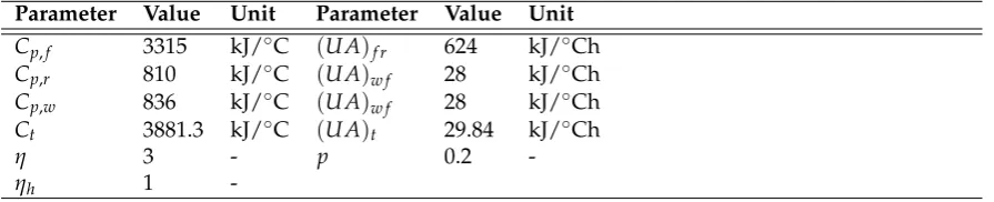
As mentioned previously, we consider heat pump and solar water heater as thermal appliances for current simulation studies. Table1contains the values of the parameters used in modelling of thermal appliances as described in [35] and [37]. To put a constraint on the indoor air temperature, (18◦C,22◦C) is specified as the desired comfort range. These constraints can be chosen to be time varying also. The heat pump is considered to consume maximum of 1 kW power at each time step. Similarly, the water temperature in the solar water heater tank is kept bounded between (50◦C,70◦C) and the maximum power consumption of the water heater is considered to be 2 kW. Everyday water withdrawal demand profile is obtained from the DHWcalc toolbox [38], which generates realistic domestic hot water demand depending upon various characteristics like number of households, total mean daily draw off volume etc.
Without any loss of generality, washing machine and dishwasher are considered as the non-thermal household appliances. Table2details the parameter values for the washing machine and the dishwasher. Every day, non-thermal appliance requests are activated at random time steps with a random deadline which is greater than the total running time of the appliance.
Table 1.Thermal appliance parameters
Parameter Value Unit Parameter Value Unit Cp,f 3315 kJ/◦C (U A)f r 624 kJ/◦Ch
Cp,r 810 kJ/◦C (U A)w f 28 kJ/◦Ch
Cp,w 836 kJ/◦C (U A)w f 28 kJ/◦Ch
Ct 3881.3 kJ/◦C (U A)t 29.84 kJ/◦Ch
η 3 - p 0.2
-ηh 1
-Table 2.Non-thermal appliance parameters
Appliance Running Time (Ω) Rated-Power (P)
Washing machine 2 Hours 3kW
Dishwasher 2.5 Hours 4 kW
The entire simulation setup is implemented in Matlab. For simulation purpose, ambient temperature Ta and solar radiation φs are obtained from ASHRAE IWEC (International Weather
for Energy Calculations) weather data files for Dublin, Ireland [39]. The electricity prices are taken from wholesale Danish Energy Market data [40] and employed for real time implementation of the proposed algorithm. A maximum capacity constraint of 4 kW is imposed on the total power consumption of all the appliances. In reality, the capacity constraints can be time varying. The setup is simulated over 7 days period with a prediction horizon of 24 hours (Mode 1). To solve the MILP, Gurobi solver is used in integration with YALMIP toolbox [41] and Matlab.
7.2. Results and Discussion
the subjected comfort zone boundaries and the constraint on the power consumption of the heat pump is also satisfied.
Similarly, Figure3presents the temperature variation of water in the water tank, and the power consumed by the water heater respectively. The initial water temperature is considered to be at 20◦C (see Figure3a). As the time passes, the temperature gradually increases over next few hours and then it is maintained inside the specified temperature range. This also explains the fact that the power consumed by the water heater is high in beginning of the simulation period in Figure3b.
Figure4aand Figure4bshows the power consumed by the washing machine and the dishwasher respectively. It can be seen that the appliances operation is interrupted occasionally in order to minimize the electricity cost and satisfy the capacity constraints. It should be noted that, the HEMS has no knowledge about the arrival request of washing-machine and dishwasher. The arrival requests are generated randomly to investigate the capability of the HEMS to handle immediate request situations.
0 20 40 60 80 100 120 140 160 180 Time [Hours] 17 18 19 20 21 22 23 Temperature [ ° C]
The Indoor Temperature
T r constraint
(a)
0 20 40 60 80 100 120 140 160 180 Time [Hours]
0 0.5 1 1.5
Power consumption [kW]
Power consumption of heat pump W
c constraint
(b)
Figure 2.(a)Room temperature with HEMS, (b)Power consumption by heat pump with HEMS
0 20 40 60 80 100 120 140 160 180 Time [Hours] 20 25 30 35 40 45 50 55 60 65 70 75 Temperature [ ° C]
Tank water Temperature
T t constraint
(a)
0 20 40 60 80 100 120 140 160 180 Time [Hours] 0 0.5 1 1.5 2
Power consumption [kW]
Power consumption of water heater P
h constraint
(b)
0 24 48 72 96 120 144 168 Time [Hours]
0 0.5 1 1.5 2 2.5 3 3.5 4
Power consumption [kW]
Power consumption of washing machine
(a)
0 24 48 72 96 120 144 168 Time [Hours]
0 0.5 1 1.5 2 2.5 3 3.5 4 4.5 5
Power consumption [kW]
Power consumption of dishwasher
(b)
Figure 4. (a) Power consumption of washing machine with HEMS, (b) Power consumption of dishwasher with HEMS
7.2.1. Without HEMS and On-Off Control for Thermal Appliances
In order to evaluate the effectiveness of the HEMS, a different scenario is considered. In this case, there is no HEMS to schedule the appliances. The thermal appliances are operated using On-Off control strategy. The thermal appliances turn-on when the temperature is below the lower threshold of the specified range. Since, there is no control over the non-thermal appliances, so once turned-on, they run continuously for their respective runtimes. Figure5ashows the total power consumption of all the appliances in this case. It can be seen that the peak power consumption is around 9 kW which occurs on the fourth day of the week.
0 20 40 60 80 100 120 140 160 180
Time [Hours]
0 2 4 6 8 10
Power consumption [kW]
Total Power Consumption
consumption capacity constraint
(a)
0 20 40 60 80 100 120 140 160 180
Time [Hours]
0 1 2 3 4 5 6 7 8
Power consumption [kW]
Total Power Consumption consumption capacity constraint
(b)
0 20 40 60 80 100 120 140 160
Time [Hours]
0 2 4 6 8 10
Power consumption [kW]
Total Power Consumption
consumption capacity constraint
(c)
7.2.2. Without HEMS and MPC Control for Thermal Appliances
The operation of thermal appliances using on-off control strategy is a basic control technique, so another different scenario is considered. Similar to the previous case, there is no HEMS to schedule the appliances in this case also. But, the thermal appliances are operated using MPC strategy which is an advanced control technique in comparison to on-off control.
Figure5b shows the total power consumption in this case. It is seen that the peak power consumption in this case is reduced to around 7.5 kW which occurs at around 12:30 PM on the fourth day. It is seen in the Figure7that all the appliances (thermal and non-thermal appliances) are in operation at this time which implies that only 0.5 kW power is consumed by the thermal appliances. This happen because the MPC has prior knowledge of the external disturbances (MPC) so it operates the appliances to comply with the subjected constraint of maximum peak-power consumption. Clearly, using MPC instead of on-off controller is useful to reduce the peak-power consumption.
7.2.3. With HEMS
In this scenario, there is HEMS employed in the house to schedule the appliances. All the appliances are scheduled using MPC strategy in this case. Figure5cclearly depicts the benefits of using HEMS and presents the total power consumed by all the household appliances. In Figure5c, it can be seen that for initial time steps, total power consumption goes beyond the capacity limit of 4 kW, which happens due to the high power consumption of water heater since initial water temperature in the tank is low. At later time steps, it can be seen that the maximum total power consumed by all the appliances stays around the capacity limit. The constraints on the capacity limit are allowed to violate to ensure the feasibility of the optimization problem (soft constraints).
Figure
6.
The
operation
schedule
of
the
appliances
without
HEMS
and
on-of
f
contr
ol
for
the
ther
mal
Figure
7.
The
operation
schedule
of
the
appliances
without
HEMS
and
MPC
contr
ol
for
the
thermal
app
Figure
8.
Operation
Schedule
of
the
appliances
with
The total electricity cost as per the time varying prices used in this study, is detailed in the Table3. In comparison to the case without HEMS and On-Off controller for the thermal appliances, a reduction of 47 % is achieved in total electricity cost by using the HEMS. Similarly, in comparison to the case without HEMS and MPC controller for the thermal appliances, the HEMS achieves a reduction of 45 %.
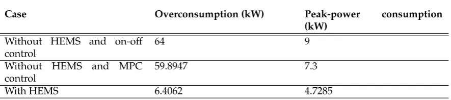
To see the effectiveness of HEMS in reducing the peak-load, the total violation of the capacity constraint over the simulation period and the maximum peak-load consumed by the appliances for all the cases is presented in Table5. The total violation for the case when appliances are scheduled with HEMS is about 10 times lower than the case of no HEMS with On-Off control and MPC control for thermal appliances. Similarly, by using HEMS, the peak power consumption is reduced by 48 % and 36% in comparison with the case of no HEMS with On-Off control and MPC control for thermal appliances respectively. The PAR for all the cases is detailed in the Table4. It is observed that by using the HEMS, PAR is reduced by 38 % and 24% in comparison to other two cases.
Table 3.The total electricity cost for the entire simulation duration
Case Electricity cost (e) Without HEMS and on-off control 8.5594
Without HEMS and MPC control 8.2005
With HEMS 4.4934
Table 4.Peak to Average Ratio
Case Peak-power
consumption (kW)
Mean-power consumption (kW)
PAR
Without HEMS and on-off control
9 1.11 8.11
Without HEMS and MPC control
7.31 1.10 6.65
With HEMS 4.7285 0.937 5.04
Table 5.Total violation of capacity contrsaint during the simulation period
Case Overconsumption (kW) Peak-power consumption
(kW) Without HEMS and on-off
control
64 9
Without HEMS and MPC control
59.8947 7.3
With HEMS 6.4062 4.7285
8. Conclusions
In this work, the problem of scheduling of appliances to achieve reduction in the peak-load and total electricity cost has been investigated using model predictive control (MPC). An architecture of a home energy management system (HEMS) is presented which operate in two modes of operations (MOOs) based upon the categorization of the appliances (thermal and non-thermal). The system dynamics of the appliances have been modelled into a state-space formulation.
the peak power consumption also. The operation schedule of appliances with and without HEMS has also been compared. The non-thermal appliances were able to interrupt and shift to the low electricity price periods while finishing the task by the deadline. The future work includes the consideration of energy storage facility, renewable energy generation and integration of plug-in electric vehicle (PEVs) into the framework. Also, the framework will be scaled up to a small community or a group of houses to investigate the demand-response from the perspective of power utility or aggregator companies.
1. Pérez-Lombard, L.; Ortiz, J.; Pout, C. A review on buildings energy consumption information. Energy and buildings2008,40, 394–398.
2. Andersen, P.B.; Hauksson, E.B.; Pedersen, A.B.; Gantenbein, D.; Jansen, B.; Andersen, C.A.; Dall, J.Smart Grid Applications, Communications, and Security; Wiley-VCH, 2012.
3. Strbac, G. Demand side management: Benefits and challenges. Energy policy2008,36, 4419–4426. 4. Albadi, M.H.; El-Saadany, E. Demand response in electricity markets: An overview. 2007 IEEE power
engineering society general meeting, 2007.
5. Palensky, P.; Dietrich, D. Demand side management: Demand response, intelligent energy systems, and smart loads.IEEE transactions on industrial informatics2011,7, 381–388.
6. Balijepalli, V.M.; Pradhan, V.; Khaparde, S.; Shereef, R. Review of demand response under smart grid paradigm. Innovative Smart Grid Technologies-India (ISGT India), 2011 IEEE PES. IEEE, 2011, pp. 236–243. 7. Brambley, M.R.; Hansen, D.; Haves, P.; Holmberg, D.; McDonald, S.; Roth, K.; Torcellini, P. Advanced
sensors and controls for building applications: Market assessment and potential R&D pathways. Pacific Northwest National Laboratory2005.
8. Stankovic, J.A. Real-time computing system: The next generation1988.
9. De Angelis, F.; Boaro, M.; Fuselli, D.; Squartini, S.; Piazza, F.; Wei, Q. Optimal home energy management under dynamic electrical and thermal constraints. IEEE Transactions on Industrial Informatics2013, 9, 1518–1527.
10. Adika, C.O.; Wang, L. Autonomous appliance scheduling for household energy management. IEEE Transactions on Smart Grid2014,5, 673–682.
11. Mohsenian-Rad, A.H.; Leon-Garcia, A. Optimal residential load control with price prediction in real-time electricity pricing environments. IEEE Trans. Smart Grid2010,1, 120–133.
12. Setlhaolo, D.; Xia, X. Optimal scheduling of household appliances with a battery storage system and coordination. Energy and Buildings2015,94, 61–70.
13. Paterakis, N.G.; Erdinc, O.; Bakirtzis, A.G.; Catalão, J.P. Optimal household appliances scheduling under day-ahead pricing and load-shaping demand response strategies. IEEE Transactions on Industrial Informatics 2015,11, 1509–1519.
14. Shirazi, E.; Jadid, S. Optimal residential appliance scheduling under dynamic pricing scheme via HEMDAS. Energy and Buildings2015,93, 40–49.
15. Sou, K.C.; Weimer, J.; Sandberg, H.; Johansson, K.H. Scheduling smart home appliances using mixed integer linear programming. 2011 50th IEEE Conference on Decision and Control and European Control Conference. IEEE, 2011, pp. 5144–5149.
16. Paridari, K.; Parisio, A.; Sandberg, H.; Johansson, K.H. Robust Scheduling of Smart Appliances in Active Apartments With User Behavior Uncertainty.IEEE Transactions on Automation Science and Engineering2016, 13, 247–259.
17. Wu, X.; Hu, X.; Yin, X.; Moura, S. Stochastic optimal energy management of smart home with PEV energy storage.IEEE Trans. Smart Grid2016, pp. 1–1.
18. Matallanas, E.; Castillo-Cagigal, M.; Gutiérrez, A.; Monasterio-Huelin, F.; Caamaño-Martín, E.; Masa, D.; Jiménez-Leube, J. Neural network controller for active demand-side management with PV energy in the residential sector. Applied Energy2012,91, 90–97.
19. Soares, A.; Antunes, C.H.; Oliveira, C.; Gomes, Á. A multi-objective genetic approach to domestic load scheduling in an energy management system.Energy2014,77, 144–152.
21. Aslam, S.; Iqbal, Z.; Javaid, N.; Khan, Z.; Aurangzeb, K.; Haider, S. Towards efficient energy management of smart buildings exploiting heuristic optimization with real time and critical peak pricing schemes. Energies2017,10, 2065.
22. Zhang, D.; Li, S.; Sun, M.; O?Neill, Z. An optimal and learning-based demand response and home energy management system. IEEE Transactions on Smart Grid2016,7, 1790–1801.
23. Ozturk, Y.; Senthilkumar, D.; Kumar, S.; Lee, G.K. An Intelligent Home Energy Management System to Improve Demand Response. IEEE Trans. Smart Grid2013,4, 694–701.
24. Setlhaolo, D.; Xia, X.; Zhang, J. Optimal scheduling of household appliances for demand response.Electric Power Systems Research2014,116, 24–28.
25. Haider, H.T.; See, O.H.; Elmenreich, W. Dynamic residential load scheduling based on adaptive consumption level pricing scheme. Electric Power Systems Research2016,133, 27–35.
26. Pipattanasomporn, M.; Kuzlu, M.; Rahman, S. An algorithm for intelligent home energy management and demand response analysis. IEEE Transactions on Smart Grid2012,3, 2166–2173.
27. Costanzo, G.T.; Zhu, G.; Anjos, M.F.; Savard, G. A system architecture for autonomous demand side load management in smart buildings. IEEE Transactions on Smart Grid2012,3, 2157–2165.
28. Rastegar, M.; Fotuhi-Firuzabad, M.; Zareipour, H. Home energy management incorporating operational priority of appliances.International Journal of Electrical Power & Energy Systems2016,74, 286–292.
29. Garcia, C.E.; Prett, D.M.; Morari, M. Model predictive control: theory and practice?a survey. Automatica 1989,25, 335–348.
30. Chen, C.; Wang, J.; Heo, Y.; Kishore, S. MPC-based appliance scheduling for residential building energy management controller. IEEE Transactions on Smart Grid2013,4, 1401–1410.
31. Rahmani-Andebili, M. Scheduling deferrable appliances and energy resources of a smart home applying multi-time scale stochastic model predictive control. Sustainable Cities and Society2017,32, 338–347. 32. Hammer, A.; Heinemann, D.; Lorenz, E.; Lückehe, B. Short-term forecasting of solar radiation: a statistical
approach using satellite data. Solar Energy1999,67, 139–150.
33. Mellit, A.; Pavan, A.M. A 24-h forecast of solar irradiance using artificial neural network: Application for performance prediction of a grid-connected PV plant at Trieste, Italy.Solar Energy2010,84, 807–821. 34. Brogan, W.L.Modern control theory; Pearson Education India, 1982.
35. Halvgaard, R.; Poulsen, N.K.; Madsen, H.; Jørgensen, J.B. Economic model predictive control for building climate control in a smart grid. 2012 IEEE PES Innovative Smart Grid Technologies (ISGT). IEEE, 2012, pp. 1–6.
36. Staino, A.; Nagpal, H.; Basu, B. Cooperative optimization of building energy systems in an economic model predictive control framework. Energy and Buildings2016,128, 713–722.
37. Halvgaard, R.; Bacher, P.; Perers, B.; Andersen, E.; Furbo, S.; Jørgensen, J.B.; Poulsen, N.K.; Madsen, H. Model predictive control for a smart solar tank based on weather and consumption forecasts. Energy Procedia2012,30, 270–278.
38. Jordan, U.; Vajen, K. DHWcalc: Program to generate domestic hot water profiles with statistical means for user defined conditions. Proceedings of the ISES Solar World Congress, Orlando, FL, USA, 2005, pp. 8–12. 39. EnergyPlus Energy Simulation Software-International Weather for Energy Calculations (IWEC) Data for Ireland.http://apps1.eere.energy.gov/buildings/energyplus/cfm/weather_data3.cfm/region=6_europe_ wmo_region_6/country=IRL/cname=Ireland. Accessed: Jun-2018.
40. Danish electricity wholesale market. http://www.energinet.dk/EN/El/Engrosmarked/Sider/default. aspx. Accessed: Jun-2018.