Diphoton searches (CMS)
MilenaQuittnat1,on behalf of the CMS collaboration
1ETH Zurich
Abstract.The search for high mass resonances decaying into two photons is well
mo-tivated by many physics scenarios beyond the standard model. This note summarizes the results of this search in proton-proton collision with a center-of-mass energy of√
s = 13 TeV and an integrated luminosity of 3.3 fb−1 by the CMS experiment. It
presents the interpretation of the results under spin-0 and spin-2 hypotheses with a rel-ative width up to 5.6×10⁻² in a mass region of 500−4500 GeV. The results of the
√s
=13 TeV analysis are combined statistically with previous searches performed by
the CMS collaboration, employing a center-of-mass energy of √s =8 TeV and an
inte-grated luminosity of 19.7 fb−1.
1 Introduction
Several extensions of the standard model (SM) of particle physics predict the production of a reso-nance decaying into a high mass photon pair. The Landau-Yang theorem postulates a spin of 0 or an integer value of higher than 2 for these resonances [1]. The analysis described focuses on two benchmark models:
• the production of a spin-0 resonance via gluon-gluon fusion.
• an extra dimensional model, the Randall-Sundrum model, predicting a spin-2 resonance.
The so called two-Higgs-doublet model (2HDM) predicts the existence of five additional scalar or pseudo-scalar particles in the Higgs sector [2]. The lightest neutral Higgs particle could be identi-fied with the 125 GeV Higgs boson which was discovered by the CMS and ATLAS experiments in
2012 [3, 4]. In the alignment limit, one of the additional neutral Higgs particles with massmS could
decay into two photons at a significant rate and be detected in the CMS or ATLAS detector [5].
Additional space-like dimensions provide an explanation for the observed difference between the
Planck and electroweak scales by introducing a gravitational field which also propagates through at least one extra dimension. The metric of the Randall-Sundrum (RS) graviton model [6] is that one of a five-dimensional anti-de-Sitter space with one warped extra-dimension. The RS-model postulates two brane worlds. The SM fields exist only on the ’electroweak brane’ whereas gravity is also allowed
e-mail: [email protected]
to propagate to the second ’gravity brane’. The mediator of the gravitational force, the graviton, might
then be observed as a spin-2 resonance with massmGin the ATLAS or CMS detector and would
de-cay, among others, into diphotons. In 2015, the ATLAS and CMS collaborations could explore a new
energy range using proton-proton collisions at a center-of-mass energy of√s=13 TeV. Both
collabo-rations presented results on searches for diphoton resonances in the mass ranges of 200 GeV−2 TeV
(500 GeV−5 TeV) for spin-0 (spin-2) hypotheses at ATLAS [7] and 500 GeV−4.5 TeV at CMS [8].
This note summarizes the results from the CMS collaboration at √s=13 TeV with an integrated
luminosity of 3.3 fb−1 and reports further on the statistical combination of this search with similar
searches by the CMS collaboration performed at √s=8 TeV. The note is based on the results
re-ported in Ref. [9].
2 Diphoton reconstruction with the CMS detector
A detailed description of the CMS apparatus, together with the relevant kinematic variables, can be found in Ref. [10]. The CMS detector is designed to include the central tracking and calorimetric
system within its solenoid, which provides a magnetic field of B=3.8 T. The muon detection system
surrounds the solenoid and is placed within the steel skeleton of the detector. The central ’barrel’ part of the detector is complemented by a forward region at each side, the so-called ’endcaps’. The reconstruction of photon candidates rely mainly one the electromagnetic calorimeter (ECAL) and to some extent on the tracker system. The electromagnetic calorimeter is built from lead-tungstate
crystals providing an excellent intrinsic diphoton energy resolution of approximately 0.5 % for masses
above 100 GeV. Photon candidates are formed by clustering spatially correlated energy deposits in ECAL. They are reconstructed by the particle-flow event algorithm [11, 12], applying an optimized combination of the information of various detector parts. The energy of the photon candidates is evaluated by a multivariate regression technique. For a detailed description of the applied calibrations, corrections and techniques, Ref. [13] may be consulted.
3 Event selection and reconstruction
The full list of the used simulation samples of this analysis can be found in Ref. [9]. The 13 TeV
datset with an integrated luminosityLof 3.3 fb−1is recorded with two different magnetic field
con-figurations: 2.7 fb−1with B=3.8 T and 0.6 fb−1 with B=0 T. The diphoton final state has a clean
experimental signature and two well isolated high momentum photon candidates. The trigger se-lection thus requires at least two photon candidates of transverse momentum above 60(40) GeV for
B=3.8 T (B=0 T) and is fully efficient for the search range of massesmX greater than 0.5 TeV [9].
For the final event selection, photon candidates are required to have a transverse momentum of
pT > 75 GeV and a pseudorapidity of|ηS C|<2.5 as well as|ηS C|<1.44 for at least one of them. To
maximize the sensitivity of the analysis, the selected events are separated into two categories:
• EBEB: both photons are centrally detected, in the barrel (EB) region of ECAL with|ηS C|<1.44.
• EBEE: one photon is centrally detected, the other one in the forward region, the endcaps (EE) of
ECAL with 1.56<|ηS C|<2.5.
The invariant massmγγ of the diphoton pair is required to be above 230 GeV (320 GeV) for EBEB
(EBEE) events. The diphoton mass resolution depends also on the vertex identification. If the
dif-ference between the reconstructed vertex and the true vertex is smaller than 1 cm, the effect on the
to propagate to the second ’gravity brane’. The mediator of the gravitational force, the graviton, might then be observed as a spin-2 resonance with massmGin the ATLAS or CMS detector and would de-cay, among others, into diphotons. In 2015, the ATLAS and CMS collaborations could explore a new energy range using proton-proton collisions at a center-of-mass energy of√s=13 TeV. Both
collabo-rations presented results on searches for diphoton resonances in the mass ranges of 200 GeV−2 TeV (500 GeV−5 TeV) for spin-0 (spin-2) hypotheses at ATLAS [7] and 500 GeV−4.5 TeV at CMS [8]. This note summarizes the results from the CMS collaboration at √s=13 TeV with an integrated
luminosity of 3.3 fb−1 and reports further on the statistical combination of this search with similar searches by the CMS collaboration performed at √s=8 TeV. The note is based on the results
re-ported in Ref. [9].
2 Diphoton reconstruction with the CMS detector
A detailed description of the CMS apparatus, together with the relevant kinematic variables, can be found in Ref. [10]. The CMS detector is designed to include the central tracking and calorimetric system within its solenoid, which provides a magnetic field of B=3.8 T. The muon detection system
surrounds the solenoid and is placed within the steel skeleton of the detector. The central ’barrel’ part of the detector is complemented by a forward region at each side, the so-called ’endcaps’. The reconstruction of photon candidates rely mainly one the electromagnetic calorimeter (ECAL) and to some extent on the tracker system. The electromagnetic calorimeter is built from lead-tungstate crystals providing an excellent intrinsic diphoton energy resolution of approximately 0.5 % for masses above 100 GeV. Photon candidates are formed by clustering spatially correlated energy deposits in ECAL. They are reconstructed by the particle-flow event algorithm [11, 12], applying an optimized combination of the information of various detector parts. The energy of the photon candidates is evaluated by a multivariate regression technique. For a detailed description of the applied calibrations, corrections and techniques, Ref. [13] may be consulted.
3 Event selection and reconstruction
The full list of the used simulation samples of this analysis can be found in Ref. [9]. The 13 TeV datset with an integrated luminosityLof 3.3 fb−1is recorded with two different magnetic field con-figurations: 2.7 fb−1with B=3.8 T and 0.6 fb−1 with B=0 T. The diphoton final state has a clean experimental signature and two well isolated high momentum photon candidates. The trigger se-lection thus requires at least two photon candidates of transverse momentum above 60(40) GeV for B=3.8 T (B=0 T) and is fully efficient for the search range of massesmX greater than 0.5 TeV [9]. For the final event selection, photon candidates are required to have a transverse momentum of pT > 75 GeV and a pseudorapidity of|ηS C|<2.5 as well as|ηS C|<1.44 for at least one of them. To maximize the sensitivity of the analysis, the selected events are separated into two categories:
• EBEB: both photons are centrally detected, in the barrel (EB) region of ECAL with|ηS C|<1.44.
• EBEE: one photon is centrally detected, the other one in the forward region, the endcaps (EE) of ECAL with 1.56<|ηS C|<2.5.
The invariant massmγγ of the diphoton pair is required to be above 230 GeV (320 GeV) for EBEB (EBEE) events. The diphoton mass resolution depends also on the vertex identification. If the dif-ference between the reconstructed vertex and the true vertex is smaller than 1 cm, the effect on the
mass resolution is negligible. For the B=3.8 T dataset, a boosted decision tree is used for the vertex
identification and the interaction vertex is correctly assigned for about 90 % of the signal events [9]. Since this approach relies on the pTof the tracks, a different identification method has to be used for
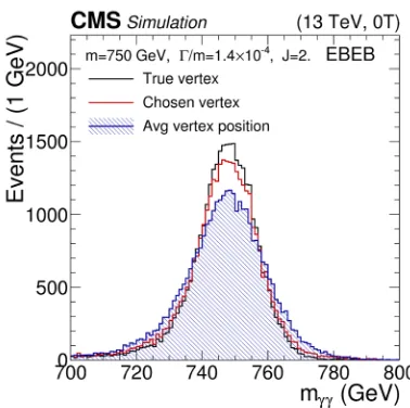
B=0 T and subsequently the vertex with the highest track multiplication is chosen. The chosen
ver-tex algorithm improves the expected mass resolution of a possible resonance by approximately 20% in comparison to the average vertex position as depicted in Figure 1. The probability for the correct vertex assignment is about 60 %.
Figure 1.Expected reconstructed invariant mass distribution for a narrow width diphoton resonance at a mass of
m=750 GeV with B=0 T for different primary vertex identifications, when both photons are centrally detected (EBEB).
For the final event selection, the photon candidates are required to satisfy a set of identification cri-teria. The respective variables and thresholds depend on the value of the magnetic field and are detailed in Ref. [9]. The per-photon identification efficiency is above 90 (85)% in the barrel (endcaps)
for B=3.8 T. In the B=0 T dataset, the per-photon identification efficiency is above 85 (70)% for
prompt isolated photon candidates in the barrel (endcaps), mainly due to a less efficient electron-veto.
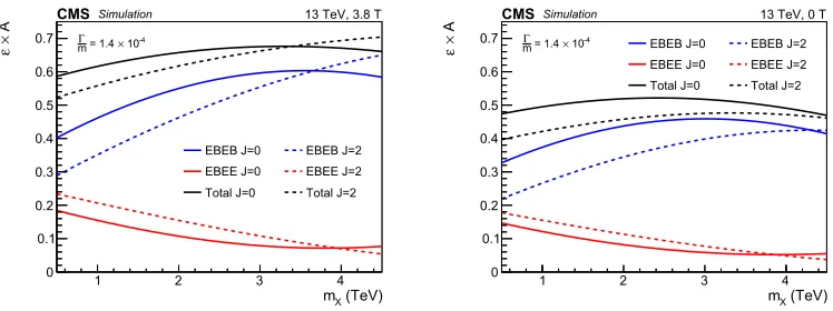
The overall signal selection efficiency as a function ofmX is shown in Figure 2 and varies between 0.5−0.7 (0.4−0.5) for B=3.8 T (B=0 T), depending on the signal hypothesis. The kinematic
ac-ceptance for the RS graviton resonances is approximately 20% lower than for scalar resonances for masses below 1 TeV due to the different angular distribution of the decay products. The two
accep-tances become similar formX >3 TeV. There is nearly no difference in the expected sensitivity for the spin-0 or spin-2 hypothesis.
A data-driven tag and probe method is employed to verify the photon selection efficiency using
Z→e+e−events. The electrons have to satisify the selection for the high momentum photon
can-didates with an inverted electron veto. The photon selection efficiency in data and the ratio to the
Monte-Carlo (MC) prediction as a function of the transverse momentumpTis shown in Figure 3. The scale factor is compatible with 1 in almost allpT-bins and flat within a few percents. A 8 (16) %
(TeV) X m
1 2 3 4
3 10
×
A
×
ε
0 0.1 0.2 0.3 0.4 0.5 0.6
0.7 = 1.4 × 10⁻⁴
m
Γ
EBEB J=0 EBEE J=0 Total J=0
EBEB J=2 EBEE J=2 Total J=2 13 TeV, 3.8 T
CMS Simulation
(TeV) X m
1 2 3 4
3 10
×
A
×
ε
0 0.1 0.2 0.3 0.4 0.5 0.6
0.7 = 1.4 × 10⁻⁴
m
Γ EBEB J=0
EBEE J=0 Total J=0
EBEB J=2 EBEE J=2 Total J=2
13 TeV, 0 T
CMSSimulation
Figure 2. Fraction of events selected by the analysis categories for a possible signal of
500 GeV < mX < 4.5 TeV andΓX/mX = 1.4× 10⁻⁴. The prediction for both, scalar and RS graviton
resonances, are shown, on the left for the B=3.8 T sample and on the right for the B=0 T one.
certainty on the selection efficiency is propagated to the signal normalization at B=3.8 T (B=0 T).
Figure 3.Photon selection efficiency measured with B=3.8 T (left) and B=0 T (right) using the tag and probe
method (all cuts are applied except for electron rejection) for the EB category. Bottom: data over Monte-Carlo scale factors.
3.1 Energy corrections
The reconstruction and energy assignment of photon candidates is generally derived for lower energy photons than the ones entering this analysis. Thus, the energy scale and energy resolution might
(TeV) X m
1 2 3 4
3 10
×
A
×
ε
0 0.1 0.2 0.3 0.4 0.5 0.6
0.7 = 1.4 × 10⁻⁴
mΓ
EBEB J=0 EBEE J=0 Total J=0
EBEB J=2 EBEE J=2 Total J=2 13 TeV, 3.8 T
CMS Simulation
(TeV) X m
1 2 3 4
3 10
×
A
×
ε
0 0.1 0.2 0.3 0.4 0.5 0.6
0.7 = 1.4 × 10⁻⁴
m
Γ EBEB J=0
EBEE J=0 Total J=0
EBEB J=2 EBEE J=2 Total J=2
13 TeV, 0 T
CMS Simulation
Figure 2. Fraction of events selected by the analysis categories for a possible signal of
500 GeV < mX < 4.5 TeV andΓX/mX = 1.4× 10⁻⁴. The prediction for both, scalar and RS graviton
resonances, are shown, on the left for the B=3.8 T sample and on the right for the B=0 T one.
certainty on the selection efficiency is propagated to the signal normalization at B=3.8 T (B=0 T).
Figure 3.Photon selection efficiency measured with B=3.8 T (left) and B=0 T (right) using the tag and probe
method (all cuts are applied except for electron rejection) for the EB category. Bottom: data over Monte-Carlo scale factors.
3.1 Energy corrections
The reconstruction and energy assignment of photon candidates is generally derived for lower energy photons than the ones entering this analysis. Thus, the energy scale and energy resolution might
need to be corrected for higher values. As the energy determination is only dependent on ECAL, well-known electron objects from Z→e+e−events can be used instead of photon objects. Residual differences in the observed and predicted distributions of a Z→e+e−sample are thus determined by
a tag and probe method with a procedure described in Ref. [13]. The energy scale corrections are about 0.5 (1.5) % for photon candidate compatibles at B=3.8 T (B=0 T). The additional Gaussian
smearing for the MC prediction is similar for both values of the magnetic field and of the order of 0.8 % and 1.5 % (2−2.5 %) for photon candidates which are centrally (in the forward region) detected. The energy scale correction factors measured for the B=0 T dataset are found to be about 1 % higher
than the B=3.8 T factors. The comparison with the MC prediction after all energy corrections are applied is reported in Figure 4. The variation of the corrections is studied with Z→e+e−events as a function of the transverse momentum pTup to 150 (100 GeV) for EB (EE). The variation is smaller than 0.5 (0.7) % for EB (EE) in both datasets.
Figure 4.Comparison between the predicted and observed invariant mass distribution of electron pairs obtained
after the application of energy scale and resolution corrections. Distributions are shown for events where both electrons are reconstructed for B=3.8 T (left) and B=0 T (right) in the EBEB category. The simulation predic-tions are scaled to match the number of events observed in data.
4 Diphoton mass spectrum
The diphoton spectrum of the events entering the analysis is shown in Figure 5 for all four categories ((B=3.8 T,B=0 T)×(EBEB,EBEE)) .
The individual background components of the diphoton sample at B=3.8 T are estimated by a
data-driven method. This evaluation measures that about 90 (80) % of the background events in the EBEB (EBEE) category originate from the irreducibleγγ-SM background processes. This estimate is
com-pared to a precise next-to-next-to leading-order (NNLO) prediction of theγγ-SM background
pro-cesses. It is obtained by calculating the so-called ’k-factor’, the ratio of the theoretical calculation of
Events / 20 GeV
1 10 2 10
Data Fit model
1 s.d.
±
2 s.d.
±
EBEB
(GeV)
γ γ m 400 600 800 1000 1200 1400 1600
stat
σ
(data-fit)/ -2 0 2
CMS
(13 TeV, 3.8 T) -1
2.7 fb
Events / 20 GeV
1 10 2
10 Data
Fit model 1 s.d.
±
2 s.d.
±
EBEE
(GeV)
γ γ m 400 600 800 1000 1200 1400 1600
stat
σ
(data-fit)/ -2 0 2
CMS
(13 TeV, 3.8 T) -1
2.7 fb
Events / 20 GeV
1 10 2
10 Data
Fit model 1 s.d.
±
2 s.d.
±
EBEB
(GeV)
γ γ m 400 600 800 1000 1200 1400 1600
stat
σ
(data-fit)/ -2 0 2
CMS
(13 TeV, 0 T) -1
0.6 fb
Events / 20 GeV
1
10 DataFit model 1 s.d.
±
2 s.d.
±
EBEE
(GeV)
γ γ m 400 600 800 1000 1200 1400 1600
stat
σ
(data-fit)/ -2 0 2
CMS
(13 TeV, 0 T) -1
0.6 fb
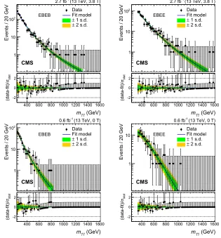
Figure 5. The observed invariant mass spectra are shown for the EBEB (left) and EBEE category (right). The
top (bottom) row shows the results for the B=3.8 T (B=0 T) dataset. The results of the parametric fits to the
data are depicted with their uncertainties.
the 2gNNLO [14] simulation program with the leading-order SHERPA simulation at gen-level. The
leading-orderγγ-prediction, a SHERPA event generator sample emulated with the detector response,
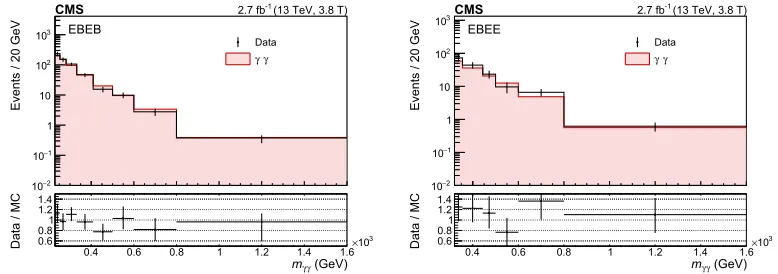
is then reweighed with this k-factor. The comparison of theγγspectrum with the NNLO MC
predic-tion is reported in Figure 6. The predicpredic-tions from perturbative QCD match the observapredic-tions within their uncertainties.
5 Statistical analysis
A simultaneous unbinned likelihood fit tomγγ evaluates the diphoton distributions in all four analysis
categories ((B=3.8 T,B=0 T)×(EBEB,EBEE)) and for each signal hypothesisS:
L(µ, θ)= ΠNevents
i=1 [µ·S(mi|θS)]+B(mi|θB)]·Poisson(Nevents|NB+µ·NS)
Events / 20 GeV 1 10 2 10 Data Fit model 1 s.d. ± 2 s.d. ± EBEB (GeV) γ γ m 400 600 800 1000 1200 1400 1600
stat σ (data-fit)/ -2 0 2 CMS
(13 TeV, 3.8 T) -1
2.7 fb
Events / 20 GeV
1 10 2 10 Data Fit model 1 s.d. ± 2 s.d. ± EBEE (GeV) γ γ m
400 600 800 1000 1200 1400 1600
stat σ (data-fit)/ -2 0 2 CMS
(13 TeV, 3.8 T) -1
2.7 fb
Events / 20 GeV
1 10 2 10 Data Fit model 1 s.d. ± 2 s.d. ± EBEB (GeV) γ γ m 400 600 800 1000 1200 1400 1600
stat σ (data-fit)/ -2 0 2 CMS
(13 TeV, 0 T) -1
0.6 fb
Events / 20 GeV
1
10 DataFit model 1 s.d. ± 2 s.d. ± EBEE (GeV) γ γ m
400 600 800 1000 1200 1400 1600
stat σ (data-fit)/ -2 0 2 CMS
(13 TeV, 0 T) -1
0.6 fb
Figure 5. The observed invariant mass spectra are shown for the EBEB (left) and EBEE category (right). The
top (bottom) row shows the results for the B=3.8 T (B=0 T) dataset. The results of the parametric fits to the data are depicted with their uncertainties.
the 2gNNLO [14] simulation program with the leading-order SHERPA simulation at gen-level. The leading-orderγγ-prediction, a SHERPA event generator sample emulated with the detector response, is then reweighed with this k-factor. The comparison of theγγspectrum with the NNLO MC predic-tion is reported in Figure 6. The predicpredic-tions from perturbative QCD match the observapredic-tions within their uncertainties.
5 Statistical analysis
A simultaneous unbinned likelihood fit tomγγevaluates the diphoton distributions in all four analysis categories ((B=3.8 T,B=0 T)×(EBEB,EBEE)) and for each signal hypothesisS:
L(µ, θ)= ΠNevents
i=1 [µ·S(mi|θS)]+B(mi|θB)]·Poisson(Nevents|NB+µ·NS)
Events / 20 GeV
2 − 10 1 − 10 1 10 2 10 3 10 Data γ γ (GeV) γ γ m
0.4 0.6 0.8 1 1.2 1.4 1.6
3 10
×
Data / MC 0.60.8 1 1.2 1.4
(13 TeV, 3.8 T) -1
2.7 fb
CMS EBEB
Events / 20 GeV
2 − 10 1 − 10 1 10 2 10 3 10 Data γ γ (GeV) γ γ m
0.4 0.6 0.8 1 1.2 1.4 1.6
3 10
×
Data / MC 0.60.8 1 1.2 1.4
(13 TeV, 3.8 T) -1
2.7 fb
CMS EBEE
Figure 6. Comparison between the predicted and measuredγγ background spectrum. Events in the EBEB
(EBEE) category are shown on the left (right).
whereBdenotes the SM background model. The signal and background model depend on the mass
mi of eventiand their respective nuisance parametersθ, which model the systematic uncertainties. The parameterµdenotes the signal strength of the considered model. The interpretation is performed
with a composite statistical hypothesis test. The test statistics are based on a profile likelihood ratio of the form:
q(µ)=−logλ(µ) :=−logL(µ·S +B|
ˆ
θµ)
L(ˆµ·S +B|θˆ)
relying on the likelihoodL. The ˆxnotation denotes the best fit value of parameterx, the notation ˆxy symbolizes the best fit value ofx, conditionally ony.
The shape of the diphoton distribution as a function ofmγγmodels the background expectation using the functional form:
g(mγγ )=mγγ a+b·log(mγγ)
The coefficients are obtained through the maximum likelihood fit to data. Independent coefficients
are used for each analysis category and are considered as unconstrained nuisance parameters. The uncertainty on the accuracy of the background determination is assessed and accounted for in the hypothesis test [9].
The signal distribution as a function ofmγγ is described as the convolution of the intrinsic shape of the resonance and the ECAL detector response [9, 19]. The signal hypotheses considered herein are simulated at leading order with the PYTHIA [20] event generator, using NNPDF 2.3 [21] parton distribution functions. Three different values of relative width are used as benchmark models:
• ΓXis much smaller than the detector resolution:ΓX/mX =1.4×10⁻⁴. • ΓXis of the same size as the detector resolution:ΓX/mX=1.4×10−2. • ΓXmuch larger than the detector resolution:ΓX/mX =5.6×10⁻².
For the RS graviton model, the relative widths correspond to the dimensionless coupling parame-ter
˜
k =
ΓX/mX
1.4 =0.01,0.1, and 0.2
as described in Ref. [22]. In order to determine the signal normalization, the efficiency of the final event selection is combined with the kinematic acceptance as shown in Figure 2. In this analysis, the statistical uncertainties dominate over the systematic ones. In addition to the above mentioned
systematics on the background model, the selection efficiency and the photon energy scale, the
luminosity uncertainty and the uncertainty on the parton distribution function enter the hypothesis test.
For the interpretation of the results, frequentist statistics and asymptotic formulas [15] are used throughout and their validity is tested [9]. Thus, upper limits on the resonant diphoton production rate
under different signal hypotheses are evaluated with the modified frequentist method, also known as
CLs[16, 17]. The agreement of the observed result with the background-only hypothesis is estimated
by the background-onlyp−value, the ’localp-value’p0[18].
6 Results of the search at
√
s
= 13 TeV
For the √s=13 TeV dataset, the search range for a possible resonance with massmX covers the
region 500 GeV<mX<4.5 TeV. The median expected and observed 95% C.L. exclusion limits
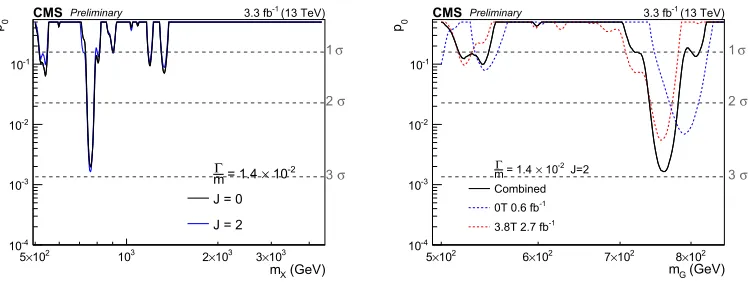
on the production of scalar and RS graviton resonances are reported in Fig. 7 for the narrow and the largest width hypotheses. The complete list of results for the exlusion limits as well as for the
background-only p−value can be found in Ref. [9]. In Figure 8, the results for a relative width of
ΓX/mX =1.4×10⁻²are shown on the left. This signal hypothesis shows the largest excess in data
among all considered widths hypotheses at a mass ofmX =760 GeV. The background-only p-value
for the RS graviton model is depicted on the right side of that figure and shows a local significance of
2.9 standard deviations. The separate B=3.8 T and B=0 T contributions point out that the B=0 T
category adds approximately 20 % to the observed excess due to its lower luminosity. The probabil-ity of observing at least one excess more significant than that in the full search range and among all
considered models of this analysis, is the so-called “look-elsewhere-effect" [23]. It is derived from a
sampling distribution of max(p0) of an ensemble of background-only pseudo datasets and found to be
less than one standard deviation.
(GeV) S m 2
10
×
5 103 2×10³ 3×10³
) (fb)
γγ
→
S
→
(pp
σ
95% C.L. limit
0 2 4 6 8 10 12 14 16 18
J=0 -4 10
×
= 1.4 mΓ Expected limit
σ
1
± σ
2
±
Observed limit (13 TeV) -1 3.3 fb
CMS Preliminary
(GeV) S m 2
10
×
5 103 2×10³ 3×10³
) (fb)
γγ
→
S
→
(pp
σ
95% C.L. limit
0 5 10 15 20 25 30 35
J=0 -2 10
×
= 5.6 mΓ Expected limit
σ
1
± σ
2
±
Observed limit (13 TeV) -1 3.3 fb
CMSPreliminary
Figure 7. Expected and observed 95% C.L. exclusion limits in the range 500 GeV<mX<4.5 TeV for
ΓX/mX = 1.4×10⁻⁴(left) and 5.6×10⁻²(right) for the scalar (J=0) resonance hypothesis.
as described in Ref. [22]. In order to determine the signal normalization, the efficiency of the final event selection is combined with the kinematic acceptance as shown in Figure 2. In this analysis, the statistical uncertainties dominate over the systematic ones. In addition to the above mentioned
systematics on the background model, the selection efficiency and the photon energy scale, the
luminosity uncertainty and the uncertainty on the parton distribution function enter the hypothesis test.
For the interpretation of the results, frequentist statistics and asymptotic formulas [15] are used throughout and their validity is tested [9]. Thus, upper limits on the resonant diphoton production rate
under different signal hypotheses are evaluated with the modified frequentist method, also known as
CLs[16, 17]. The agreement of the observed result with the background-only hypothesis is estimated
by the background-onlyp−value, the ’local p-value’p0[18].
6 Results of the search at
√
s
= 13 TeV
For the √s=13 TeV dataset, the search range for a possible resonance with massmX covers the
region 500 GeV<mX <4.5 TeV. The median expected and observed 95% C.L. exclusion limits
on the production of scalar and RS graviton resonances are reported in Fig. 7 for the narrow and the largest width hypotheses. The complete list of results for the exlusion limits as well as for the
background-only p−value can be found in Ref. [9]. In Figure 8, the results for a relative width of
ΓX/mX =1.4×10⁻² are shown on the left. This signal hypothesis shows the largest excess in data
among all considered widths hypotheses at a mass ofmX =760 GeV. The background-only p-value
for the RS graviton model is depicted on the right side of that figure and shows a local significance of
2.9 standard deviations. The separate B=3.8 T and B=0 T contributions point out that the B=0 T
category adds approximately 20 % to the observed excess due to its lower luminosity. The probabil-ity of observing at least one excess more significant than that in the full search range and among all
considered models of this analysis, is the so-called “look-elsewhere-effect" [23]. It is derived from a
sampling distribution of max(p0) of an ensemble of background-only pseudo datasets and found to be
less than one standard deviation.
(GeV) S m 2 10 ×
5 103 2×10³ 3×10³
) (fb) γγ → S → (pp σ
95% C.L. limit
0 2 4 6 8 10 12 14 16 18 J=0 -4 10 × = 1.4 m Γ Expected limit σ 1 ± σ 2 ± Observed limit (13 TeV) -1 3.3 fb CMS Preliminary (GeV) S m 2 10 ×
5 103 2×10³ 3×10³
) (fb) γγ → S → (pp σ
95% C.L. limit
0 5 10 15 20 25 30 35 J=0 -2 10 × = 5.6 mΓ Expected limit σ 1 ± σ 2 ± Observed limit (13 TeV) -1 3.3 fb CMS Preliminary
Figure 7. Expected and observed 95% C.L. exclusion limits in the range 500 GeV<mX <4.5 TeV for
ΓX/mX = 1.4×10⁻⁴(left) and 5.6×10⁻²(right) for the scalar (J=0) resonance hypothesis.
(GeV) X m 2 10 ×
5 103 2×10³ 3×10³
0 p -4 10 -3 10 -2 10 -1 10 -2 10 × = 1.4 mΓ J = 0 J = 2
σ 1 σ 2 σ 3 (13 TeV) -1 3.3 fb CMS Preliminary (GeV) G m 2 10 ×
5 6×10² 7×10² 8×10²
0 p -4 10 -3 10 -2 10 -1 10 J=2 -2 10 × = 1.4 mΓ Combined -1 0T 0.6 fb
-1 3.8T 2.7 fb
σ 1 σ 2 σ 3 (13 TeV) -1 3.3 fb CMSPreliminary
Figure 8. Observed background only p-values obtained on the 13 TeV,dataset. ForΓX/mX = 1.4×10⁻², the
range 500 GeV < mX < 4.5 TeV (850 GeV) is shown on the left (right). Results corresponding to both spin hypotheses are shown on the left. The contributions of the B=3.8 T and B=0 T datasets are shown separately
on the right for the spin-2 hypothesis. Due to the different integrated luminosity, the weight of the B=0 T dataset
atmX=760 GeV is approximately 20 % of the B=3.8 T one in the combined result.
7 Results of the combined analysis of
√
s
= 8 TeV and 13 TeV
datasets
The results of the √s = 13 TeV dataset are combined statistically with results obtained by the
CMS collaboration at a center-of-mass energy of √s = 8 TeV employing an integrated
luminos-ity of 19.7 fb−1. Two searches for resonant diphoton production were performed with the 8 TeV
dataset:
• an analysis searching for spin-0 and spin-2 resonances in the mass range 150−850 GeV [24].
• a second analysis focusing on spin-2 resonances with a search range of 500 GeV−3 TeV [25].
The two event samples partially overlap, thus at eachmX, the analysis with the most stringent median
expected exclusion limit on resonant diphoton production is taken for the final combination. For
resonance masses belowmX <850 GeV, the results of Ref. [24] enter the combination, and those of
Ref. [25] otherwise. The ratio of the signal production cross sections at 8 TeV and 13 TeV has been calculated [9]. It is approximately
• 0.29 (0.27) formG(mS)=500 GeV,
• 0.24 (0.22) formG(mS)=750 GeV,
• 0.04 (0.03) for masses in the TeV range (mGormS ≈3 TeV).
For further details, Ref. [9] may be consulted. The combined result is obtained by a
simulta-neous fit to the mγγ spectra in all event categories, assuming a common signal strength modifier
for all categories. The median expected and observed 95% CLsexclusion limits on the equivalent
13 TeV diphoton resonance production cross section, σ13 TeVG,S · Bγγ, for the combined analysis are
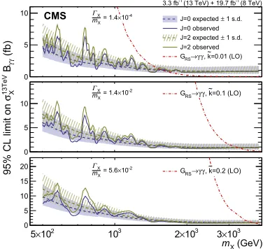
reported in Figure 9 for all studied signal hypothesis of this analysis. The comparison with
Fig-ure 7 shows an improvement of the exclusion limits by 20−40 % for masses below 1.5 TeV. For
masses above 1.5 TeV, the exclusion limits are mainly driven by the sensitivity of the 13 TeV
anal-ysis and the benefits of the combination decrease. Randall-Sundrum gravitons with masses below approximately 1.6, 3.3, and 3.8 TeV are excluded at a 95 % confidence level for ˜κ = 0.01,0.1,
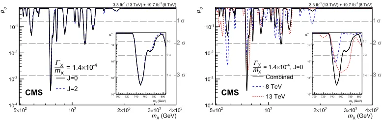
and 0.2, respectively, corresponding to a relative widths of ΓX/mX = 1.4 ×10−4,1.4 × 10−2 and 5.6 ×10⁻². Similar exclusion limits are found for the scalar signal hypotheses. The re-sult of the local significance for a scalar resonance under the narrow width hypothesis is de-picted in Figure 10. This model shows the largest excess in the combination among all consid-ered signal hypotheses with a local significance of roughly 3.4 standard deviations at a mass of
mS =750 GeV. Further results can be found in Ref. [9]. Taking into account the effect of search-ing for a diphoton resonance among all six signal hypotheses, the global significance is estimated to be approximately 1.6 standard deviations [9].
(GeV) X
m
2 10
×
5 103 2×10³ 3×10³ 0
5 10 15
20 =5.6×10⁻² GRS→γγ,k~=0.2 (LO)
X
mX
Γ
0 5 10
=0.1 (LO) k~ ,
γ γ →
RS
G
-2
10
×
1.4 =
X
mX
Γ
0 5
10 J=0 expected ± 1 s.d.
J=0 observed 1 s.d.
±
J=2 expected J=2 observed
=0.01 (LO) k ~ ,
γ γ →
RS
G
-4
10
×
1.4 =
X
mX
Γ
(fb)γγ
B
13TeV Xσ
95% CL limit on
CMS
(8 TeV)
-1
(13 TeV) + 19.7 fb
-1
3.3 fb
Figure 9.Expected and observed 95% C.L. exclusion limits in the range 500 GeV<mX<3 TeV for both spin
hypothesis with a relative width ofΓX/mX = 1.4×10⁻⁴(top),ΓX/mX = 1.4×10⁻²(middle) andΓX/mX = 5.6×
10−2(bottom).
8 Summary and outlook
This note summarizes the search for high mass resonances decaying into the diphoton final state by the CMS experiment [9]. The analysis employs a dataset of 3.3 fb−1 and 19.7 fb−1of proton-proton collisions at a center-of-mass energy of √s = 13 TeV and √s = 8 TeV, respectively. The
search sets 95% CLsexclusion limits on the resonant diphoton production of scalar resonances (J=0) and RS gravitons (J= 2) in the mass range of 500 GeV < mX < 4.5 TeV for relative width up toΓX/mX =5.6×10⁻², using leading-order simulation for the signal processes. Randall-Sundrum gravitons with masses below approximately 1.6, 3.3, and 3.8 TeV are excluded at a 95 % confidence level for ˜κ = 0.01,0.1,and 0.2, respectively, corresponding to a relative widths ofΓX/mX = 1.4× 10−4,1.4×10−2and 5.6×10⁻². A modest excess of events over the background-only hypothesis is observed formX =750 GeV. The corresponding local significance under the narrow-width hypothesis
(ΓX/mX = 1.4×10⁻⁴) for a spin-0 particle is approximately 3.4 standard deviations. Taking into
masses above 1.5 TeV, the exclusion limits are mainly driven by the sensitivity of the 13 TeV
anal-ysis and the benefits of the combination decrease. Randall-Sundrum gravitons with masses below approximately 1.6, 3.3, and 3.8 TeV are excluded at a 95 % confidence level for ˜κ = 0.01,0.1,
and 0.2, respectively, corresponding to a relative widths of ΓX/mX = 1.4 × 10−4,1.4 × 10−2 and 5.6 ×10⁻². Similar exclusion limits are found for the scalar signal hypotheses. The re-sult of the local significance for a scalar resonance under the narrow width hypothesis is de-picted in Figure 10. This model shows the largest excess in the combination among all consid-ered signal hypotheses with a local significance of roughly 3.4 standard deviations at a mass of
mS =750 GeV. Further results can be found in Ref. [9]. Taking into account the effect of search-ing for a diphoton resonance among all six signal hypotheses, the global significance is estimated to be approximately 1.6 standard deviations [9].
(GeV) X m 2 10 ×
5 103 2×10³ 3×10³ 0
5 10 15
20 =5.6×10⁻² GRS→γγ,k~=0.2 (LO)
X mX Γ 0 5 10 =0.1 (LO) k~ , γ γ → RS G -2 10 × 1.4 = X mX Γ 0 5
10 J=0 expected ± 1 s.d.
J=0 observed 1 s.d. ± J=2 expected J=2 observed =0.01 (LO) k ~ , γ γ → RS G -4 10 × 1.4 = X mX Γ (fb)γγ B
13TeV Xσ
95% CL limit on
CMS
(8 TeV)
-1
(13 TeV) + 19.7 fb
-1
3.3 fb
Figure 9.Expected and observed 95% C.L. exclusion limits in the range 500 GeV<mX <3 TeV for both spin
hypothesis with a relative width ofΓX/mX = 1.4×10⁻⁴(top),ΓX/mX = 1.4×10⁻²(middle) andΓX/mX = 5.6×
10−2(bottom).
8 Summary and outlook
This note summarizes the search for high mass resonances decaying into the diphoton final state by the CMS experiment [9]. The analysis employs a dataset of 3.3 fb−1 and 19.7 fb−1of proton-proton collisions at a center-of-mass energy of √s = 13 TeV and √s =8 TeV, respectively. The
search sets 95% CLsexclusion limits on the resonant diphoton production of scalar resonances (J=0)
and RS gravitons (J = 2) in the mass range of 500 GeV < mX < 4.5 TeV for relative width up toΓX/mX =5.6×10⁻², using leading-order simulation for the signal processes. Randall-Sundrum gravitons with masses below approximately 1.6, 3.3, and 3.8 TeV are excluded at a 95 % confidence level for ˜κ = 0.01,0.1,and 0.2, respectively, corresponding to a relative widths ofΓX/mX = 1.4× 10−4,1.4×10−2and 5.6×10⁻². A modest excess of events over the background-only hypothesis is observed formX=750 GeV. The corresponding local significance under the narrow-width hypothesis
(ΓX/mX = 1.4×10⁻⁴) for a spin-0 particle is approximately 3.4 standard deviations. Taking into
(GeV) X m 2 10 ×
5 103 2×10³ 3×10³ 4×10³
0 p -4 10 -3 10 -2 10 -1
10 1σ
σ 2 σ 3 -4 10 × 1.4 = X mX Γ J=0 J=2 (GeV) X m
700 720 740 760 780 800
0 p -4 10 -3 10 -2 10 -1
10 1σ
σ 2 σ 3 (8 TeV) -1
(13 TeV) + 19.7 fb
-1 3.3 fb CMS (GeV) X m 2 10 ×
5 103 2×10³ 3×10³ 4×10³
0 p -4 10 -3 10 -2 10 -1
10 1σ
σ 2 σ 3 , J=0 -4 10 × 1.4 = X mΓX
Combined 8 TeV 13 TeV (GeV) X m
700 720 740 760 780 800
0 p -4 10 -3 10 -2 10 -1
10 1σ
σ 2 σ 3 (8 TeV) -1
(13 TeV) + 19.7 fb
-1
3.3 fb
CMS
Figure 10. Left: observed background-only p-values obtained on the 8 and 13 TeV combination for both spin
hypothesis and a relative width ofΓX/mX = 1.4×10⁻⁴. Right: observed background-only p-values for the spin-0
hypothesis with a relative width ofΓX/mX = 1.4×10⁻⁴. The contributions of the 8 and 13 TeV datasets are
shown separately.
account all signal hypotheses considered in the analysis, the global significance of this excess is estimated to 1.6 standard deviations.
References
[1] L.D. Landau, Dokl. Akad. Nauk SSSR60, 207 (1948)
[2] N. Craig, J. Galloway, S. Thomas (2013),1305.2424
[3] G. Aad et al. (ATLAS), Phys. Lett.B716, 1 (2012),1207.7214
[4] S. Chatrchyan et al. (CMS), Phys. Lett.B716, 30 (2012),1207.7235
[5] P.S.B. Dev, A. Pilaftsis (2014),1408.3405
[6] L. Randall, R. Sundrum, Phys. Rev. Lett.83, 3370 (1999),hep-ph/9905221
[7] Journal of High Energy Physics2016, 1 (2016)
[8] CMS Collaboration (CMS), CMS Physics Analysis Summary CMS-PAS-EXO-15-004 (2015),
https://cds.cern.ch/record/2114808
[9] V. Khachatryan et al. (CMS Collaboration), Phys. Rev. Lett.117, 051802 (2016)
[10] S. Chatrchyan et al. (CMS), JINST3, S08004 (2008)
[11] CMS Collaboration (CMS), CMS Physics Analysis Summary CMS-PAS-PFT-09-001 (2009),
http://cdsweb.cern.ch/record/1194487
[12] CMS Collaboration (CMS), CMS Physics Analysis Summary CMS-PAS-PFT-10-001 (2010),
http://cdsweb.cern.ch/record/1247373
[13] V. Khachatryan et al. (CMS), JINST10, P08010 (2015),1502.02702
[14] S. Catani, L. Cieri, D. de Florian, G. Ferrera, M. Grazzini, Phys.Rev.Lett.108, 072001 (2012),
1110.2375
[15] G. Cowan, K. Cranmer, E. Gross, O. Vitells, Eur.Phys.J.C71, 1554 (2011),1007.1727
[16] T. Junk, Nucl. Instrum. Meth. A434, 435 (1999),hep-ex/9902006
[17] A. Read, Tech. Rep. CERN-OPEN-2000-005, CERN (2000),
http://cdsweb.cern.ch/record/451614
[18] ATLAS and CMS Collaborations, LHC Higgs Combination Group, ATL-PHYS-PUB/CMS
NOTE 2011-11, 2011/005 (2011),http://cdsweb.cern.ch/record/1379837
[19] M. Baak, S. Gadatsch, R. Harrington, W. Verkerke, Nucl. Instrum. Meth. A771, 39 (2015),
1410.7388
[20] T. Sjöstrand, S. Ask, J.R. Christiansen, R. Corke, N. Desai, P. Ilten, S. Mrenna, S. Prestel, C.O.
Rasmussen, P.Z. Skands, Comput. Phys. Commun.191, 159 (2015),1410.3012
[21] R.D. Ball et al., Nucl. Phys.B867, 244 (2013),1207.1303
[22] H. Davoudiasl, J.L. Hewett, T.G. Rizzo, Phys. Rev. Lett.84, 2080 (2000),hep-ph/9909255
[23] E. Gross, O. Vitells, Eur. Phys. J.C70, 525 (2010),1005.1891
[24] V. Khachatryan et al. (CMS), Phys. Lett.B750, 494 (2015),1506.02301
[25] CMS Physics Analysis Summary CMS-PAS-EXO-12-045, CERN (2015),
http://cds.cern.ch/record/2017806