Available Online at www.ijcsmc.com
International Journal of Computer Science and Mobile Computing
A Monthly Journal of Computer Science and Information Technology
ISSN 2320–088X
IJCSMC, Vol. 4, Issue. 4, April 2015, pg.96 – 105
RESEARCH ARTICLE
PROBABILISTIC PATH QUERIES IN NETWORKS PATH:
EFFICIENT AND EFFECTIVE CLUSTERING METHODS
R.BRINDHA, M.E, CSE (PT), SCSVMV, KANCHIPURAM, [email protected]
MRS.V.GEETHA, M.E, AP, DEPARTMENT OF CSE, SCSVMV KANCHIPURAM, [email protected]
MRS.T.JAYANTHI, M.E AP, DEPARTMENT OF CSE, SCSVMV, KANCHIPURAM, [email protected]
ABSTRACT
Correlations may exist among adjacent edges in various probabilistic graphs. As one of the basic mining techniques, graph clustering is widely used in exploratory data analysis, such as data compression, information retrieval, image segmentation, etc. Graph clustering aims to divide data into clusters according to their similarities, and a number of algorithms have been proposed for clustering graphs, such as the pKwikCluster algorithm, spectral clustering, k-path clustering, etc. To develop efficient clustering algorithms for probabilistic graphs it becomes more challenging to efficiently cluster probabilistic graphs when correlations are considered. In this paper, we define the problem of clustering correlated probabilistic graphs. To solve the challenging problem, we propose two algorithms, namely the PEEDR and the CPGS clustering algorithm. For each of the proposed algorithms, we develop several pruning techniques to further improve their efficiency.
Index Terms—Clustering, correlated, probabilistic graphs, algorithm
1. INTRODUCTION
probability of existence. As an example, consider the probabilistic protein-protein interaction (PPI) networks.
In a probabilistic graph, any two edges ei and ej are called conditionally independent if p(ei, ej)
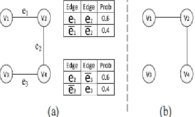
= p(ei)p(ej), and conditionally dependent if p(ei, ej) ≠p(ei)p(ej). For the standard probabilistic graph model, any two edges are conditionally independent of each other. Typically, coexistence and mutual exclusion among adjacent edges are commonly observed in various graph oriented applications. For example, in Fig. 1(a), given two edges e2 and e3 with a mutual exclusion constraint, only the joint probabilities p(e2, e3) and p(e2, e3) may exist, where ei represents that ei does not exist. Obviously,
p(e2, e3) ≠p(e2)p(e3), and hence e2 and e3 are conditionally dependent on each other. Similarly, e1 and e2 are also conditionally dependent on each other due to a coexistence Constraint, correlations will lead to incorrect results.
Define the probabilistic graphs containing correlated adjacent edges as correlated probabilistic graphs as shown in Fig.2(a). As one of the basic data mining techniques, clustering is widely used in
Fig. 1. Graph model: (a) Probabilistic graph with edge correlations.(b) Possible world graph.
Fig.2. Correlated probabilistic graph and a cluster graph: (a) Correlated probabilistic graph.(b) Cluster graph.
•We formally define the problem of clustering correlated probabilistic graphs and investigate related properties.
• We propose a new algorithm, PEEDR, which is rather efficient for clustering correlated probabilistic graphs, and several pruning methods for this algorithm.
• We develop an algorithm, CPGS, for clustering correlated probabilistic graphs based on the spectral clustering algorithm, which can produce better cluster.
2. RELATED WORK
2.1 Algorithms for Clustering Deterministic Graphs
Deterministic graph clustering has been extensively studied in data mining research and a number of clustering algorithms have been developed. Ahmed et al. [1]. The different categories of clustering algorithms and recent efforts to design clustering methods for various kinds of graph data Jain et al. [7]As one of the most widely used graph clustering algorithms, spectral clustering has received increased interest of researchers. Spectral clustering relies on the eigen structure of a graph Laplacian matrix to partition vertices into disjoint clusters, with points in the same cluster having high similarity and points in different clusters having low similarity [9].
2.2 Querying and Mining of Probabilistic Graphs
Many classical data mining problems have been redefined in probabilistic graphs, such as the reachability query, shortest path query, K-NN query, etc. Jin et al. [3] studied the Distance-constraint Reachability query and presented a sampling algorithm to answer the NP-hard problem.
2.3 Querying and Mining the Probabilistic Data with Correlations
An efficient strategy was developed for query evaluation over such probabilistic databases by casting the query processing problem as inference problem in an appropriately constructed probabilistic graphical model. Lian et al. [16] investigated the nearest neighbor query on uncertain data with local correlations. Tight lower and upper bounds of the subgraph similarity probability were developed to prune the search space. Compared to these queries, clustering over correlated probabilistic graphs is more complicated.
3. PROBLEM DEFINITIONS
Define the model of a correlated probabilistic graph as G = {V, E, P, F}, where V is the set of vertices, E
is the set of edges, P is the existence probability, and F is the joint probability distribution of edges. The output graph is modeled as a cluster graph which is composed of several disconnected clusters and each vertex in the graph only belongs to one cluster.
In this model, the joint probability distribution F is of the form f (e1, e2, · · · , ek) = p, where ei denotes existence, ei denotes non existence for edge ei ∊ E, and p is the value of the joint probability.
A possible world graph serves as efficient probabilistic graphs. For a correlated probabilistic graph G = {V, E, P, F}, a possible world graph Gi = {V' , E'} is an instantiation sampled from G, where V'= V and E'cE.
4. PEEDR CLUSTERING ALGORITHM
4.1 Basic PEEDR Clustering Algorithm
Definition 1 (Adjacent Vertex to Cluster).
Consider a graph G = {V, E, P, F}, and a cluster C in the cluster graph Q of G. Let VC denote the set
of nodes in cluster C. For any vertex v ∊ V \ VC, that vertex v is adjacent tothe cluster C if it is adjacent to at
least one vertex in VC, denoted as v ∊ Adj(C).
The PEEDR algorithm initializes a cluster with one vertex. Then for each vertex that is adjacent to the cluster, it is removed into the cluster if it reduces the expected edit distance from G to the current cluster graph. The above step is iteratively applied until we cannot expand the cluster. Next choose a vertex from the unclustered vertices and repeat the above procedure to generate another cluster. The procedure is repeated until all vertices of G are grouped into clusters. Consequently, get the final cluster graph. One open problem in the above clustering procedure is which vertex to choose in each iteration.
PEEDR algorithm is outlined in Algorithm 1. The algorithm first sorts all the vertices in descending order of their degrees (Line 1). It next initializes a virtual cluster C', where VC'= {v|v ∊V}, which keeps all
the clustered vertices (Line 3). The algorithm finds the vertex with the maximum degree in VC', denoted as v' (Line 5). As an optimization of our algorithm build a Distance-Probability-Threshold Clique DPTC centered at v', denoted as Ci(Line 6). The algorithm will check each vertex vj ∊VC' that is adjacent to Ci and put vjinto
Ci if it can reduce the objective function
D(G,Q) (Lines 9 ~ 15).
4.2 Optimizations for Clustering Process
4.2.1 Grouping Vertices into DPTCs(GVD
) Inspired by the concept of maximum clique, to build a Distance-Probability-Threshold Clique
(DPTC) centered at the singleton cluster. The intuition behind DPTC is that vertices with small distances and high similarities are likely to be grouped into the same clusters. The clustering process of the PEEDR
algorithm starts from a local graph and establishes the cluster graph gradually. As vertices will never be separated once grouped into a cluster, it is essentially a greedy algorithm.
Definition 2 (DPTC).
Given a distance threshold dt and a probability threshold α, we define a subgraph C of G as a
Distance-Probability-Threshold Clique (DPTC), if for any pair of vertices vi, vj ∊ VC, there exists a route rk
Algorithm 2 describes how to establish a DPTC. Given a distance threshold dt and a probability threshold α, we start from the original DPTC C which contains only one vertex (Line 1). For each vertex vj ∊ VC' ∩ Adj(C), if for any vertex vj ∊ VC, there exists a route rk from vi to vj that makes drk (vi, vj) ≤ dt and simrk (vi, vj) ≥ α, then vi will be added to the DPTC. The above steps are iteratively executed until no vertices meet the requirement (Lines 3~17).
isReduceEdit (Algorithm 3) and several optimization techniques (Sections 4.2.2 and 4.2.3). Then we update the set VC' = VC' \ VCi and create the next cluster from the vertices in the virtual cluster
C'. The procedure is repeated until all the vertices in C' are grouped into disconnected clusters.
4.2.2 Pruning By Loose Bounds of Objective Function(PLB)
In line 9 of Algorithm 1, for each vertex vj ∊ VC'∩Adj(Ci),we need to check whether vj should be moved from the virtual cluster C'to Ci. This is determined by D0(G,Q1)−D0(G,Q2), where Q1 and Q2 are cluster graphs, and Q2 is obtained from Q1 by moving vj from C' to Ci. If
D0(G,Q1)−D0(G,Q2) ≥ 0, vj will be moved from C' to Ci; otherwise, vj remains in C'. However, computing D0(G,Q1) and D0(G,Q2) according to the definition of estimated expected edit distance is highly complex. Instead of calculating D0(G,Q1) and D0(G,Q2), To estimate
those changed edges is < e1, e2, . . . , em >. The partial estimated expected edit distance from
G to a cluster graph Q is defined by
Then, we have
4.2.3 Pruning By Tight Upper Bounds of Objective Function (PTUB)
A tighter upper bound of the partial expected edit distance in this section.Suppose the O0
order of those edges that have changed from Q1 to Q2 is < e1, e2, . . . , em >. For any cluster graph
Q, the partial expected edit distance D0p (G,Q) is defined in Section 4.2.2.
4.2.4 Optimizing By Redefining Objective Function (OROF)
In the proposed algorithms, joint probability tables are repeatedly read when calculating the edges’ conditional probabilities.
5. CPGS CLUSTERING ALGORITHM
Spectral clustering refers to a class of techniques which rely on the eigen-structure of a graph Laplacian matrix to partition vertices into disjoint clusters with high intra-cluster and low inter-cluster similarity.
Based on this observation, one straightforward approach to extending the spectral clustering algorithm for correlated probabilistic graphs works as follows:
1) We map conditional probabilities into weights between each pair of adjacent vertices.
2) We extend the Dijkstra method to find the K nearest neighbuor (K-NN) of each vertex. It enumerates part of the possible world graphs and calculates the probability that avertex is the K -NN of the others when correlations exist among edges
3) We establish a Laplacian matrix according to the K-NN results, and compute the eigenvectors of it according to the power method.
4) We represent the vertices by points in a K-dimensional space, and cluster these points with a
K-means algorithm. We call the straightforward method Spectral, and it will be used as a benchmark method in our experiments.
5.1 Establishing DPTCs
In the CPGS algorithm, cluster a graph by establishing DPTCs and representing these DPTCs as objects to be clustered. This can improve the time efficiency as the number of objects to be clustered is much smaller than the number of vertices. This paper represents vertices in the graph by points in a multi-dimensional space as the distance between vertices in graphs is complex to calculate compared with points in a multi-dimensional space.
5.2 Searching the K-NN of each DPTC
In CPGS, we need to find the K nearest neighbor (KNN) DPTCs of each DPTC to establish a graph Laplacian matrix. Before presenting the approaches to finding the KNN DPTCs, we define the similarity between two adjacent DPTCs based on the definition of estimated expected edit distance.
Given a correlated probabilistic graph G = {V, E, P, F}, and two adjacent DPTCs Ci and
pk(XD(ep)), where S(Ci,Cj) is the set of edges between Ci and Cj in the correlated probabilistic graph, and XD(ep) is the existence state of epin the DPTC graph GD.
5.3 Establishing a Laplacian Matrix and Calculating Eigenvectors
In this subsection, how to establish a Laplacian matrix from the graph matrix W and an approach to calculating its eigenvectors. The K eigenvectors corresponding to the K largest eigenvalues of the Laplacian matrix are used to represent each object, namely DPTC in our algorithm, with a point in a multi-dimensional space .
First how to establish a symmetric Laplacian matrix L(G) from W. Set Wij =
Max{Wij,Wji}, and thus W is a symmetric matrix. Then, a diagonal matrix D can be obtained, where Di= ΣjWij. Subsequently, we have the Laplacian matrix L(G) = D −W.
6. EXPERIMENTS 6.1 Experimental Setup
The algorithms are implemented in Microsoft Visual Studio C++ on a PC with a 4 dual core CPU and 8GB memory. Use two real-life graph datasets in our experiments.
PPI network: Use a PPI network from the STRING database[4]. The network is modeled as a probabilistic graph by representing proteins as vertices, pairwise interactions as edges, and the reliability of each pairwise interaction as edge probability. This graph has 4, 179 vertices and 39,
309 edges.
YouTube social network: In the YouTube social network1, each vertex represents a user and an edge between two vertices represents there exists a connection between them. This dataset comprises 1, 134, 890 vertices and 5, 987, 624 edges. The edge existence probability is randomly generated to indicate the link reliability between users.
Correlation Simulation: These two datasets do not contain the correlation probabilities among adjacent edges. To generate these probabilities, we first present several definitions. For the m
adjacent edges, define the correlation rate θ among these edges sharing the same vertex, so that the correlation only exists among └mθ┘ edges, and the other edges are independent of each other.
6.2 Performance of PEEDR Clustering Algorithm
Evaluate the performance of the PEEDR algorithm and its optimizations.
Efficiency of Optimizations: This set of experiments studies the effect of the optimizations for
PEEDR in terms of the running time. Specifically, we compare the following algorithms:
BASIC: The PEEDR algorithm that is based on the DPTCs and does not employ any other optimizations proposed in Section 4.2.
OPSV: The difference of OPSV from the BASIC algorithm is that OPSV sorts vertices in descending order of their degrees.
PLB: Based on the OPSV algorithm, PLB adopts the pruning technique proposed in Section 4.2.2.
PTUB: Based on the PLB algorithm, the PTUB algorithm adopts the pruning technique in Section 4.2.3.
OROF: The PEEDR algorithm implemented with all the pruning techniques proposed in Section 4.
Fig. 4(a) and 4(b) report the efficiency of the different optimizations by varying the data size
from 800 to 4, 000 on PPI and YouTube
The effectiveness of PEEDR: Evaluate the effectiveness of the PEEDR algorithm. The BASIC algorithm may generate different cluster graphs from the other algorithms. In other words, PLB, PTUB and OROF do not affect the effectiveness of the PEEDR algorithm. Thus, we only discuss the effectiveness of the BASIC and the OPSV algorithms.
Fig. 6(a) and 6(b) show the accuracy rate by varying the vertex number from 800 to 4000 on PPI and YouTube networks. The accuracy decreases as the vertex number increases, since the larger the vertex number, the bigger the deviation of the generated cluster graph from the optimal cluster graph is.
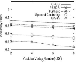
6.4 Comparisons with Existing Methods
Fig. 13 reports the accuracy rate of different algorithms. The accuracy rate decreases as the vertex number increases. We can see that CPGS and PEEDR generate better cluster graphs than the Furthest algorithm, the Girvan-Newman algorithm and the spectral clustering algorithm do.
7. CONCLUSION
In this paper, we have addressed the problem of clustering correlated probabilistic graphs and propose an efficient clustering algorithm named PEEDR. Based on the properties of joint probability, introduce several pruning methods for PEEDR. To achieve better effectiveness of clustering and also propose another clustering algorithm named CPGS. A comprehensive performance evaluation verifies the efficiency and effectiveness of our algorithms and pruning methods.
REFERENCES
[1] C. C. Aggarwal and H. Wang, Managing and Mining Graph Data,New York, NY, USA: Springer, 2010.
[2] M. Potamias, F. Bonchi, A. Gionis, and G. Kollios, ―K-nearest neighbors in uncertain graphs,‖ PVLDB, vol. 3, no. 1,pp. 997–1008, Sept. 2010.
[3] R. Jin, L. Liu, B. Ding, and H. Wang, ―Distance-constraint reachability computation in uncertain graphs,‖ PVLDB, vol. 4, no. 9, pp. 551–562, Jun. 2011.
[4] Y. Yuan, G. Wang, L. Chen, and H. Wang, ―Efficient subgraph similarity search on large probabilistic graph databases,‖ PVLDB, vol. 5, no. 9, pp. 800–811, May 2012.
[5] M. Hua and J. Pei, ―Probabilistic path queries in road networks:Traffic ncertainty aware path selection,‖ in Proc. 13th Int. EDBT,New York, NY, USA, 2010, pp. 347–358.
[6] W. C. Wang and L. A. Demsetz, ―Model for evaluating networks under correlated uncertainty-NETCOR,‖ J. Constr. Eng. Manage.,vol. 126, no. 6, pp. 458–466, 2000.
[7] A. K. Jain, M. N. Murty, and P. J. Flynn, ―Data clustering:A review,‖ ACM Comput. Surv., vol. 31, no. 3, pp. 264–323, 1999.
[8] G. Kollios, M. Potamias, and E. Terzi, ―Clustering large probabilistic graphs,‖ IEEE Trans. Knowl. Data Eng., vol. 25, no. 2,pp. 325–336, Feb. 2013.