Passive Sonar Target Detection Using Statistical Classifier and Adaptive Threshold

Article

Passive Sonar Target Detection Using Statistical

Classifier and Adaptive Threshold

Hamed Komari Alaie 1_{, Hassan Farsi 1}

1 _{Department of Electrical and Computer Engineering, University of Birjand, Birjand, Iran}

* Correspondence: [email protected]; Tel.: +985632202104

Abstract: This paper presents the results of an experimental investigation about target detecting with passive sonar in Persian Gulf. Detecting propagated sounds in the water is one of the basic challenges of the researchers in sonar field. This challenge will be complex in shallow water (like Persian Gulf) and noise less vessels. Generally, in passive sonar the targets are detected by sonar equation (with constant threshold) which increase the detection error in shallow water. Purpose of this study is proposed a new method for detecting targets in passive sonars using adaptive threshold. In this method, target signal (sound) is processed in time and frequency domain. For classifying, Bayesian classification is used and prior distribution is estimated by Maximum Likelihood algorithm. Finally, target was detected by combining the detection points in both domains using LMS adaptive filter. Results of this paper has showed that proposed method has improved true detection rate about 27% compare other the best detection method.

Keywords: Passive Sonar; Target Detection; Adaptive Threshold; Bayesian Classifier; K-Mean; Particle Filter

1.Introduction

Due to the severe attenuation of radio frequency and optical signals under the sea, the use of audio signals is often a great way to detect under water targets. Sonar (Sound Navigation and Ranging) is a technique that uses sound propagation to navigate, communicate with or detect objects on or under the surface of the water, such as other vessels. These systems record the sound waves using hydrophone and by processing these signals, we can detect, locate and classify different targets. Sonar is divided into two families of active and passive that in the active type, by sending sound pulses (pings) and analyzing the echoes of them, we can identify the type, distance and direction of the target. In the passive sonar, which is the topic of the project, underwater acoustic signals received by the hydrophone and after pre-processing, signal can be detected by analyzing the content of the target. The passive sonars use waves and their unwanted vibrations to identify vessels. The waves do not generate only from the vessels so the factors such as noise, vibrations from the bottom of sea, fishes and so on cause confusion in the detection of them. Therefore, in order to detect, we need an intelligent adaptive threshold level that at the different situations and environmental parameters to minimize error detection. Typically, the detection of sonar targets is performed using sonar equations. These equations have many variables, such as the source level, the transmission path loss, reflection lose, sound absorption and so on that some of them are the functions of other variables. In this method, which in known as the most classic detection algorithm, using Gaussian density function the mixed signal to noise and noise density threshold level detection are selected. Figure 1 shows the relationship between the various components of the hydrophone sonar arrays and decisions about the presence/absence of target.

Figure 1. basic of Target Detection in passive sonar [1]

Target detection with passive sonar has found so interesting for many researchers during last ten years. Later, in [1] performed a combined experimental and numerical study to investigate Sonar Equation for calculate signal to noise ratio. Nielsen in [2] reported that DEMON (Detection Envelope Modulation On Noise) narrowband analysis that furnishes the propeller characteristic: number of shafts, shaft rotation frequency and blade rate of the target. Martino performed LOFAR (Low Frequency Analysis and Recording) broadband analysis, estimates the noise vibration of the target machinery in frequency domain [3]. Dawe reported in [4] that using ROC curve improve target

detection performance in Sonar Equation. Chin et al. performed Two-Pass Split-Windows (TPSW)

algorithm and Neural Network to classify under water signal [5]. Borowski and et al. in [6] investigated

analysis under water signal in frequency domain. Abarahm performed non-Gaussian function for

determines Detection Threshold (DT) in [7]. Wakayama et al. describes the forecasting of probability of

target presence in a search area [8] (also referred to as the PT map) considering both detection and

non-detection conditions. Moura et al. in [9] performed independent component analysis for detect and

classify signals against background noise. Kil Woo et al. describes DEMON algorithm for detecting

target in passive sonar [10]. In [11] focused on the performance of the normalized matched filter (NMF). The NMF is used when the noise covariance matrix is fast time-varying and is hard to estimate. Zhishan Zhao et al. proposed an improved matched filter in AWGN combined with the adaptive line enhancer by

analyzing the output spectrum and the spectral spectrum of the matched filter, which is the

frequency-domain adaptive matched filter. This method is proposed for active sonar [12]. In paper [13] Mel frequency

Cestrum Coefficients feature extraction using sound pressure and particle velocity signals are researched.Firstly,

MFCC feature, first-order-differential MFCC feature, and second-order differential MFCC feature can be used as the effective feature of the underwater target identification from the feature extraction and recognition results.

Secondly, by calculating the Fisher-ratio and correlated distance, it can be found that the contribution of each dimension feature is different, and those three features fused by using fdc criterion can improve the recognition probability of underwater target signal.

The proposed method in [14] to handle the nonlinearity between target states and the raw bearing measurements, particle filter is employed to compute the joint multi target probability density (JMPD) recursively through a Bayesian framework.

In this papera new method for detecting targets in passive sonars using adaptive threshold is

proposed. In this method, target signal (sound) is processed in time and frequency domain. For classifying, Bayesian classification is used and prior distribution is estimated by Maximum Likelihood

algorithm. Finally, target was detected by combining the detection points in both domains using LMS1

adaptive filter. The chapter is organized as it follows. In Section 2, we describe proposed novel algorithm for target detection with passive sonar in shallow water. In section 3, we discuss about method of calculate detection point in time and frequency domain and fusion to determine adaptive threshold and advantages. In section 4 present the experimental results. Finally, we conclude the proposed method in Section 5 and present attempt a critical evaluation.

2.Target detection in passive sonar

Target detection, is as the separation of a special signal that's "target" from the other signals. In other words, in the case of detection, all received signals are divided into target and non-target classes by classifier. In general, non-target signals are noises and a successful classifier is one that using existing knowledge (or without special knowledge) extracts target signal from the noise.

Over the years’ researchers have used several classifiers to extract target signal from noise, such as SVM, neural networks, and statistical classifier. In this article, according to the statistical of the environment of the sea and the condition of targets (which are the mostly floating) Bayesian statistical classifier method has been used. In the proposed method, after pre-processing, the Bayesian filter is trained by the target signal and noise in time and frequency domain. For calculating the coefficients of

prior distribution ML2 _{algorithm is used. Results of Bayesian classification in each domain are recorded}

as detection point and fusion is done by Winer adaptive filters. Finally, the appropriate adaptive threshold for detection is calculated. Briefly, the proposed method is shown in Figure 2 In the following, ambient noise, radiation noise and also detail of proposed method and its results is presented.

Figure 2. Block diagram of proposed method

2.1.Ambient noise

The noise that is received by an Omni-directional hydrophone in the underwater heterogeneous environments is the ambient noise. Ambient noise level is measured by an Omni-directional hydrophone from the noise power ratio to the Omni-directional base plate hydrophone. Sources of underwater noise emissions in the environment have a bandwidth of 1 Hz to 100 KHz, which cover all frequency-existing. In order to examine the factors affecting ambient noise according to depth, the noise can be divided into two categories in deep-water and shallow water noise.

2.2.Radiated noise

Ships, submarines and torpedoes are among the sources of radiated noise. This type of noise includes machinery radiated noise, ship propeller noise and hydrodynamic noise emission. Noise

caused by turbulence, that’s caused by floatingpropeller and water bubbles floating in the back of the

vessel are broadband, and often gives cover to 10 kHz. However, the volume of this noise is under 3 kHz. Sonar noise is not white, but it is mixed with strong frequency components (above the noise level). These components are caused by the fact that, for example, in floating motor pistons, camshafts and blade-butterfly are moving out with a certain velocity relative to each other, and create slim but strong frequency components that depending on the engine speed, their power is different from each other.

3.Statistical classifier and adaptive thresh

The base of this research is detected incognito sounds. Perhaps a sound of glass or an unknown object that drops on the ground dark and silence room be a good example to express the main idea of this article. In this study, each sound divided to environment sound (which is called ambient noise) and target sound. These sounds are compared by the recorded ambient noise (training signal) and their similarities will be determined numerically by detection points. In following how to calculate detection point is described.

As shown in Figure 2, to reduce the input noise, a median filter is applied. So, Bayesian classification algorithm has been used to classify signal from noise in both time and frequency domains. The result of classification is averaged at the time domain and then the detection points are calculated. In the frequency domain (like time domain), the signal passes through the low-pass filter, then after classify by Bayesian classification, detection point is calculated by averaging. Final detection point is obtained after fusion detection points in time and frequency domains by adaptive Wiener filter.

3.1.Detection point in time domain

In this study, Bayesian algorithm is used to classify input signal. The target and noise signal have pseudo-Gaussian distribution, so applying Bayesian algorithm has shown good results for extracting the target signal. To classify the target signal, the statistical distribution of the target signal and noise

are estimated using training data. In this algorithm, if θ represents label of target (S), noise (b) and x be

a member of the input vector of the sound signal, the posterior distribution π θ( ) _{the probability of noise}

and the target, Gaussian density function f x( | )θ _{is the probability of the x value occurrence in the region}

of θ and the prior distributionp( | )θ x _{is defined by (1):}

( ) ( | ) ( | )

( ) ( | ) ( ) ( | )

f x

p x

s f x s b f x b

π θ θ

θ

π π

=

+ ₍₁₎

The Gaussian density function f x( | )θ _{is calculated by (2):}

2 2

1

( | ) ( , )

i i i

i

f x θ ω_θN μ σ_{θ θ}

=

=



(2)

In this study, to estimate the density function f x( | )θ , ML algorithm is proposed. in following this

algorithm is explained (3):

( )

{

(

) (

)

}

( )

{

(

) (

)

}

(

)

i i i i

t t t t

s i s i i s i i i

k k k k

j k

ij

k k k k

j t N k k ij j s N k k ij j k j s N

k k k

ij j k j s x Z x Z N Z x N Z x N θ θ θ θ θ θ θ θ θ θ θ θ θ θ ω σ σ μ ω σ σ μ ω μ ω σ μ ω − − − − = + = + + = + + = − = − = = = −









Finally, by estimate prior distribution and based on (4) similar target signal (H ) is separated

from ambient noise (H ).

0 1 1 ( | ) 2 1 ( | ) 2

if p s x A ccept H if p s x A ccept H

 >     _{≤ }  (4)

As mentioned, the classifier is performed in time and frequency domains. In the time domain, after classifier input signal (with lengths 10 thousand samples) into two classes of 0 (noise) and 1 (target), the resulting output has much continuity and discontinuity in some areas which due to the statistical similarity of target signal with noise. To solve the problem, the signal integrity characteristic of the target is used. In other words, the target signal has sectional continuity which is also due to the continuous movement of the vessel propeller in the water. The marine diesel engines are turned on and off with bare-speed and thus a sharp break doesn’t occur in the propeller’s sound.

Thus, the result of classification is averaged by a windows with a width of w=1000 which is

selected experimentally and it is stored in a vector called mean vector a. In (5) how calculation this

( 1) 1

1 2

1 _{( ) 1}

[ ... ]

i w

i

k i w

n w

n

a x k i

w w

a a a a

×

= − +

= ≤ ≤

=



 (5)

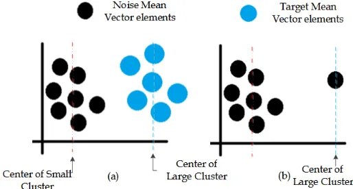
For calculation detection point, K-mean clustering algorithm is used. In this method considering

K-mean clustering algorithm, vector a is divided to two clusters, target and non-target. In Bayesian

classifier, target label is selected 1 and non-target is selected 0, so in this paper larger center of the two clusters that is closer to 1 is selected as detection point (Figure 3(a)). According to a survey conducted,

it is a necessary condition that the center of cluster is close to 1, but it is not sufficient. As shown in

Figure 3(b) it is possible noise signal has similarity in the behavior of target signal, thus in the noise signal (without present target) the value of large cluster is close to 1, which is possible due to the nature of noise, so detection point increased incorrectly.

Figure 3. Center of noise and target cluster,(a) large center is selected as detection point and (b) large center is selected as detection point incorrectly

In this study to solve this issue (Figure 3(b)), value of larger cluster center and number of its members determine detection point. If the center of each cluster is larger (close to 1) and number of members is more, the signal is similar to target and detection point increase. In (8) how calculate detention point in time domain is expressed.

2 Mt ,0 1

ttp Mt Mt

t

n

a c c

n

 

= ×  ≤ ≤

  ₍₈₎

Where the detection point in time domain for per 1000 samples is a_ttp, the larger cluster center is

Mt

c _{,the number of its members is} nMt and the whole number of members is nt. Because of the number

of cluster in K-mean algorithm is 2, to correct the error clustering of signals without any noise equation is multiplied by 2. In summary, Figure 4 shows how to calculate detection point in time domain.

Figure 4. How to calculate detection point in time domain

3.2.Detection point in frequency domain

Input signal (10 thousand samples) after passing through a low pass filter and use Fourier transformation will be separated into two cluster: 0 (noise) and 1 (target). The sound of vessel is in the lower band, so the low-pass filter is proposed.

Output of filter is averaged by a windows with a width of w=100 (which is selected

experimentally) and it is stored in a vector called mean vector A. Then with using K-mean Clustering

1 _{2 ,0 1} 3

Mf

ftp Mf Mf

f

n

A c c

n

  

= _ + _ ≤ ≤

 

  ₍₉₎

Where the detection point for per 100 samples in frequency domain is Aftp, the larger cluster center

is cMt, the number of its members is nMt, and the whole number of members is nt. Because of the number

of cluster in K-mean algorithm is 2, to correct the error clustering of signals without any noise equation is multiplied by 2. In summary, Figure 5 shows how to calculate detection point in frequency domain.

Figure 5. How Calculate detection point in frequency domain

3.3.Target Detection

As shown in Figure 2 for target detection, detection point is calculated in the time and frequency domains and the sum of these two values will determine the final detection point. If condition (10) satisfied the target is detected.

1

1 R

ttp ftp

ttp ftp

if a A Accept Target

if a A eject Target

+ ≥ 

 

+ < 

 ₍₁₀₎

With respect to condition (10), sum of two detection points directly, may increase the error detection. This fault usually is created due to climate change, air and water, the location of the sonar and etc. In this paper, to reduce the error rate, detection point in both time and frequency domain has been fused by weigh. The weights are calculated by Wiener filter.

It is worth noting for optimum weighting, Winer filter is applied as many times because of changing environmental conditions and with new environment noise signal. Figure 6 indicated How calculation adaptive detection point by Winer filter.

Figure 6. The fusion of detection points in both time and frequency domains

In this study, the Wiener filter coefficients w and W (is shown in (11)) is calculated by LMS method.

1 2

1 2

[ ... ]

[ ... ]

m m

i i

ttp ttp ttp ttp

ftp ftp ftp ftp

i ttp i ftp

i

a a a a

A A A A

DP w a W A i m

= _



= _

 =



 

(11)

Where

a



sample length in each sequence) in time domain, attp_iis the detection point of ith sequence in m

sequences in time domain, Aftp



is detection point in m sequence of test input signals in frequency

domain, Aftp_iis the detection point for ith sequence in m sequences in frequency domain, w and W are

the Wiener filter coefficients and DP is detection point after fusion. In this case the condition (10)

1 2 1

R 2

if DP Accept Target

if DP eject Target



≥ 

 

 _{< }

 ₍₁₂₎

In other words, to estimate the target signal, m sequence of input signal (test) is investigated and

eventually checking detection points in m sequences, the presence or absence of the target is

determined.

4.Experimental and simulation results

In this study, for simulating and analyzing the performance of the proposed method the database available on the Noah Institute (Copyright) is used. This database contains commercial vessels’ sound and Persian Gulf’s environmental noise. In this study, using actual environmental noises and the sound of the propeller detection is performed and the results compared with conventional methods of detection sonar equations. The following steps are simulated and the proposed method compared with conventional methods.

4.1.Simulation steps

According to Figure 2 the results of the proposed method is expressed on a database that includes pre-processing, classifying, averaging, fusion and finally detecting. In the first database is described, then the results are expressed.

4.2.Database

In the database of Noah Institute 25 unique voices of propellers of commercial vessels such as oil tankers for 30 to 120 seconds and 15 ambient noises (sound of waves of the sea, rain ...) for 10 to 30 seconds are present. As well as 25 real audio signals which contain vessels and environmental noise some of them are more than one vessel and move at different distances.

These sounds have been recorded by hydrophone at a depth of 10 meters and environmental noise when there is no vessel in a specified distance exists is recorded. Environmental noises, including sound of sea waves, sound of sea floor, the sound of rain and more. As mentioned the vessels are tankers, merchant ships and etc. In this study, the input (Background noise) to over 10 thousand sample sounds division and a sampling rate is 44 Kbps. It is worth noting the signal after the normalization is used. Figure 7 is an example of propeller sound. Figure 8 shows an example of ambient noise signal. In database, the target training signals, due to their proximity to the hydrophone have little noise. In his words, the target signals themselves are mixed with ambient noise which is the nature of underwater sound. Figure 9 shows an example of the mixed sounds (noise and the target), For example, in sample number 500 thousand a vessel in 3 km distance and sample 1 million another vessels at a distance of 8 km exist.

Figure 7. propeller sound of a commercial vessel with sampling rate 44 kHz

Figure 8. sample of ambient noise with sampling rate 44 kHz

0 2 4 6 8 10 12

x 104 -0.02

-0.015 -0.01 -0.005 0 0.005 0.01 0.015 0.02

0 0.5 1 1.5 2 2.5 3 3.5 4 4.5 5 x 105

Figure 9. sample of the mixed sounds (ambient noise and propeller sound)

To train the Bayesian algorithm and LMS, signal of environmental noise and target with 10 thousand samples have been used. The training signals are made up of noise and the target signal (mixed with noise) that the first 5 thousand samples are ambient noise and the second 5 thousand samples are the mixed signals. In some cases, to the complexity, the withe nose is added to the ambient noise.

4.3.The simulation results

The median filter is applied normalized input signal (Figure 8) and some low and high frequency noises are removed. The reason of using this filter is some high-frequency noise on the input signal.

The result is shown in Figure 10.

Figure 10. result of median filter

After applying the median filter, the output signals are divided to a sequence of signal with 10 thousand sample length. Bayesian algorithm is applied on these signals in both Fourier and time domain.

In the time domain to train the Bayesian algorithm, two groups of the target signal and ambient noise signals are used. According to the input signal mean and variances values of prior function is calculated. In the frequency domain signal input is passed from low-pass filter and after calculating the Fourier coefficient as proposed in the time domain, main and variance values of the prior function are calculated. After determining the values in time and frequency domains, detection points will be calculated by fusion. Following how calculation the detection point and simulation results is expressed.

4.4.Calculation of detection points in the time domain

After applying Bayesian algorithm in the time domain, the output will be labeled with 1(target) and 0(noise). An example of this category is shown in Figure 11.

0 0.5 1 1.5 2 2.5 3 3.5 4 4.5 5

x 105 -0.02

Figure 11.Bayesian algorithm output, in sample of 50 thousand and 100 thousand target is present (red ellipse)

To reduce classification error of Bayesian algorithm, the labeled signals are averaged by window

width w samples. The averaged values recorded at the center of the window provides a mean vector.

Figure 12 shows an example of this vector. In this method w = 5000 is selected and the average value

measured are at the center of the window. Since the input test signal length as much as 10 thousand

sample (n = 10000) and the width of the window, consuming an average of 5 thousand (w = 5000)

sample, the sample size of the vector has been reduced to 20. As shows in Figure 12 because of present target form 5 thousand, detection point is increased after sample number 10.

Figure 12. Average vector a, detection point is increased after 10 samples

As shown in Figure 4, the clustering algorithm K-mean has been used for average vector. The result is shown in Figure 13. In this figure, dots are the first cluster, crosses are the second cluster and the hollow circles are the cluster center.

Figure 13.clustering results of K-mean, dots are the first cluster, crosses are the second cluster and the hollow circles are the cluster center.

0 2 4 6 8 10 12 14 16 18 20

0 0.1 0.2 0.3 0.4 0.5 0.6 0.7 0.8 0.9 1

Sample

D

et

ec

tio

n P

oin

t

0

2

4

6

8

10

12

0 0.2 0.4 0.6 0.8 1

Nu

m

be

r

In Figure 13 the larger cluster’s center (close to 1) is 0.8 and the number of its members is 8 (from 20). According to the proposed algorithm the detection point is calculated by the equation (2), Table 1 shows detection point of 19 test signals in a specific sequence in the time domain.

Table 1.Detection point of 19 test signals in a specific sequence in the time domain

ttp

a

Type No.

0.71 Ship Engine 1

1

0.56 Ship Propeller 1

2

0.33 Ship 1

3

0.59 Ship Engine 2

4

0.62 Ship 2

5

0.59 Ship Engine 3

6

0.53 Ship Engine 4

7

0.46 Ship Engine 5

8

0.77 Ship Engine 6

9

0.26 Ship Propeller 2

10

0.56 Ship Engine 7

11

0.64 Ship Engine 8

12

0.65 Ship Engine 9

13

0.58 Ship Engine 10

14

0.46 Ambient Noise 1

15

0.44 Ambient Noise 2

16

0.53 Ambient Noise 3

17

0.51 Ambient Noise 4

18

0.26 Ambient Noise 5

19

Figure 14 shows the vector attp



for four test input signals (No.13 to 16) in the time domain.

Figure 14. vector attp

 _{for two target signals (13 and 14) and two ambient noise signals (15 and 16) in the time domain.}

4.5.Calculation of detection points in the frequency domain

The calculation of detection points in the frequency domain is similar to the proposed method in time domain, but as shown in Figure 5 the input signal is passed through a 2 kHz low-pass filter. Then Fourier coefficient is calculated with 2 thousand samples. As explained, the width of averaging

window is selected 100 (w = 100) so the length of the vector A will be the average with 20 samples.

As shown in Figure 15 because of present target in low frequency, first term coefficients is larger than

other. After the calculation of vector A, as is shown in Figure 5 the detection points are calculated in

frequency domain. Table 2 shows an example of the detection points for 19 test input signals.

0 10 20

0.55 0.6 0.65 0.7 0.75 0.8 Sample D et ec tio n P oin t V ec to r in T ime D om ain No.13

0 10 20

0.5 0.55 0.6 0.65 0.7 0.75 Sample D et ec tio n P oin t V ec to r in T ime D om ain No.14

0 10 20

0.1 0.15 0.2 0.25 0.3 0.35 0.4 0.45 0.5 0.55 0.6 Sample D et ec tio n P oin t V ec to r in T ime D om ain No.15

0 10 20

Figure 15.Mean vectorA

Table 2.detection points for 19 test input signals in a specific sequence in the frequency domain

ftp

A Type

No.

0.37

Ship Engine 1 1

0.51

Ship Propeller 1 2

0.38

Ship 1 3

0.40

Ship Engine 2 4

0.61

Ship 2 5

0.83

Ship Engine 3 6

0.41

Ship Engine 4 7

0.43

Ship Engine 5 8

0.40

Ship Engine 6 9

0.41

Ship Propeller 2 10

0.48

Ship Engine 7 11

0.59

Ship Engine 8 12

0.41

Ship Engine 9 13

0.36

Ship Engine 10 14

0.34

Ambient Noise 1 15

0.37

Ambient Noise 2 16

0.84

Ambient Noise 3 17

0.29

Ambient Noise 4 18

0.07

Ambient Noise 5 19

Figure 16 shows the vector Aftp



for four test input signals (No.13 to 16).

Figure 16.vector A_ftp for two target signals (13 and 14) and two ambient noise (15 and 16)

0 5 10 15 20

0 0.2 0.4 0.6 0.8 1 sample D et ec tio n P oin t

0 10 20

0.395 0.4 0.405 0.41 0.415 0.42 0.425 0.43 0.435 Sample Det ec tio n P oi nt V ec tor i n F req ue nc y D om ai n No.13

0 10 20

0.335 0.34 0.345 0.35 0.355 0.36 0.365 0.37 0.375 Sample Det ec tio n P oi nt V ec tor i n F req ue nc y D om ai n No.14

0 10 20

0.32 0.33 0.34 0.35 0.36 0.37 0.38 0.39 Sample Det ec tio n P oi nt V ec tor i n F req ue nc y D om ai n No.15

0 10 20

4.6.Fusion

In this paper, two methods for fusion detection point in the time and frequency domains are expressed. In the first method, detection points in these two domains are directly combined. As stated before, in this method the detection error is increased due to environmental conditions. Figure 17 shows the average of 20 sequences (m = 20) for 19 test signals (1 to 14 target signals and 15 to 19 are

the ambient noise signals). As shown in Figure 17 (Fusion Domain), the distance between the DP of

target and noise is very small and close to the threshold 1 and this caucuses to increase the detection error.

Figure 17. Average of 20 (m = 20) sequences for 19 test signals (1 to 14 are target signals and 15 to 19 are ambient noise signals)

The second method which is shown in Figure 6, the combination of weighed detection points in the time domain and frequency are performed. These weights are calculated by adaptive LMS algorithm. In this way, the number of iterations is 100 thousand, the step is 0.2 and for training three signals as environmental noise and three signals as the target are used. Figure 18 shows learning curves of the LMS adaptive filter for the cases under test.

Figure 18. learning curves of the LMS adaptive filter for the cases under test

Figure 19 shows result of the fusion by the adaptive filter. As be seen the distance between the

target and noise DP is more than the first method (Figure 17 (fusion domain)) and this will reduce the

detection error.

Figure 19. DP for 19 test signals (1 to 14 are the target signals and 15 to 17 are only ambient noise).

0 5 10 15 20

0 0.1 0.2 0.3 0.4 0.5 0.6 0.7 0.8 0.9 1 Sample D P A ver ag e 2 0 s eque nc e of T es t S ign al Time Domain Threshold Noise Target

0 5 10 15 20

0 0.1 0.2 0.3 0.4 0.5 0.6 0.7 0.8 0.9 1 Sample Frequency Domain Threshold Noise Target

0 5 10 15 20

0 0.2 0.4 0.6 0.8 1 1.2 1.4 1.6 1.8 2 Sample Fusion Domain Threshold Noise Target

100 ₁₀1 ₁₀2 ₁₀3 ₁₀4 ₁₀5 ₁₀6

0 0.2 0.4 0.6 0.8 1 1.2 1.4 1.6 1.8 2 Iteration e 2(n ) LMS

0 5 10 15 20 0 0.1 0.2 0.3 0.4 0.5 0.6 0.7 0.8 0.9 1 Sample D P A verag e 20 s eq uen ce o f T es t S igna l Time Domain Threshold Noise Target

0 5 10 15 20 0 0.1 0.2 0.3 0.4 0.5 0.6 0.7 0.8 0.9 1 Sample Frequency Domain Threshold Noise Target

5.Discussion and Conclusions

In this paper, a novel algorithm for target detection in time and frequency domain is proposed. In order to compare, the results of this method are compared with three general and practical passive sonar detection methods as sonar equation [15], detection based on the DEMON and independent component analyze (ICA) [9] and target detection based on TPSW and neural networks [5] are

expressed briefly in the following.

Sonar equation is the basic method for calculation detection threshold. The equation for

determining the performance of passive sonar is DT =SL TL− −

₍

₎

TL is the transmission loss, NL is the noise level, DI is the directivity index of the array (an

approximation to the array gain) and DT is the detection threshold. In this paper optimum DT is

selected by receiving operating characteristics (ROC) curve. Table 4 shows the values of parameters of sonar equation in the Persian Gulf.

Table 3. value of parameters of sonar equation in the Persian Gulf

SL TL NL DI Parameter

31.9 90 19.02 200 Value (dB)

In [9], for target detection, DEMON analysis is applied. DEMON algorithm is a narrow-band filter that reduces the ambient noises. Then output signal are performed over the independent sources (ICA). The ICA provides a linear representation of non-Gaussian data, so that components are statistically independent, or as much independent as possible.

The detection method is described in [5],In the preprocessing and feature extraction stage, TPSW

algorithm is used to extract tonal features from the average power spectral density. In the

classification stage, neural network classifiers are used to evaluate the classification results, inclusive of the hyper plane based Classifier-Multilayer Perceptron (MLP).

To compare proposed method with the three expressed methods same database is used. In this investigation, three categories of test data are considered. The first category includes vessels with small size and fast (eg. barges), the second category includes medium vessels (eg. cart) and third includes large vessels with low speed.

The same database is used to compare the proposed approach with the three methods expressed. Three types of test data are considered in investigation. The first category includes small sizes and slow commercial vessels (eg. barges), the second one is average speed vessels (including cart) and third includes large vessels with low speed.

Figure 20 show ROC curve compares the result of the proposed algorithm and method expressed in [15], [9] and [5] applied on same database. It is seen in Figure 20 that result of proposed method (adaptive fusion) is obviously better than other methods.

Figure 20.ROC Experimental results for target detection

As shown in Table 4, the true detection rate is 57.75% , 64.27% ,73% and 35.71% for [5], [9] and [15]

respectively whereas for the proposed method is 85.2%. The results show that proposed method has improved true detection rate about 27% compare other the best detection method.

0 0.2 0.4 0.6 0.8 1 0

0.1 0.2 0.3 0.4 0.5 0.6 0.7 0.8 0.9 1

False Positive Rate

T

ru

e Po

si

tiv

e R

ate

Detection ROC

Table 4. True detection rate

The method described in [15] (Sonar Equation) The method

described in [9] (DEMON) The method

described in [5] (TPSW NN) Proposed method

(Adaptive Fusion) Detection Method

database

25.36% 51.12%

60.35% 80.05%

First category

23.85% 48.2%

44.26% 72.63%

Second division

46.35% 69.12%

63.57% 93.85%

Third division

35.71% 61.27%

58.75% 85.2%

Total

References

1. R. J. Urick, Principles of Underwater Sound (3rd Edition), Washington, USA: McGraw-Hill, 1983.

2. R. O. Nielsen, Sonar Signal Processing, MA: Artech House Inc., 1991.

3. J. C. D. Martino, J. P. Haton and A. Laporte, "Lofargram line tracking by multistage decision," in

Speech, and Signal Processing,, USA, 1993.

4. R. L. Dawe, "Detection Threshold Modelling Explained," DSTO Aeronautical and Maritime Research Laboratory, Melbourne, Australia, 1997.

5. C. Chin Hsing, J. Der Lee and M. Chi Lin, "Classification of Underwater Signals Using Neural

Networks," Tamkang Journal of Science and Engineering, vol. 3, no. 1, pp. 31-48, 2000.

6. B. Borowski, A. Sutin, H. Seol Roh and B. Bunin, "Passive acoustic threat detection in estuarine

environments," Optics and Photonics in Global Homeland Security IV, vol. 6945, no. 1, pp. 1-11,

2008.

7. D. A. Abraham, "Detection-Threshold Approximation for Non-Gaussian Backgrounds," IEEE

Journal of Oceanic Engineering, vol. 35, no. 2, pp. 1-11, 2010.

8. Y. W. Cherry, J. G. Doug and B. Z. Zelda, "Forecasting Probability of Target Presence for Ping

Control in Multistatic Sonar Networks using Detection and Tracking Models," in 14th

International Conference on Information Fusion, Chicago, USA, 2011.

9. N. N. d. Moura, J. M. d. Seixas and R. Ramos, "Passive Sonar Signal Detection and Classification

Based on Independent Component Analysis," in Sonar Systems, Rijeka, Croatia, INTECH, 2011, pp.

93-104.

10. K. Chung, A. Sutin, A. Sedunov and M. Bruno, "DEMONAcoustic Ship SignatureMeasurements in

an Urban Harbor," Hindawi Publishing Corporation Advances in Acoustics and Vibration, vol. 11,

no. 5, pp. 1-13, 2011.

11. R. Diamant, "Closed Form Analysis of the Normalized Matched Filter With a Test Case for

Detection of Underwater Acoustic Signals," Access IEEE, vol. 4, no. 1, pp. 8225-8235, 2016.

12. Z. Zhishan, Z. Anbang, H. Juan, H. Baochun, S. Reza and N. Fang, "A Frequency-Domain Adaptive

Matched Filter for Active Sonar Detection," sensors, vol. 17, no. 1, pp. 1-12, 2017.

13. Z. Lanyue, W. Di, H. Xue and Z. Zhongrui, "Feature Extraction of Underwater Target Signal Using

Mel Frequency Cepstrum Coefficients Based on Acoustic Vector Sensor," Journal of Sensors, vol.

2016, no. 1, pp. 1-11, 2016.

14. X. Luxiao, L. Chengyuan and Y. Wei, "A particle filter based track-before-detect procedure for

towed passive array sonar system," in 2017 IEEE Radar Conference , Seattle,WA, 2017.

15. A. Ekimov and J. M. Sabatier, "Human detection range by active Doppler and passive ultrasonic

methods," in Proc. SPIE 6943, Sensors, and Command, Control, Communications, and Intelligence

(C3I) Technologies for Homeland Security and Homeland Defense VII, Bellingham, WA, USA, 2008.