The Variable Plot Method for Estimating Shrub Density.

(1)

WATER-BELLY IN STEER8 IN RELATION TO RANGE 111

phosphorus were higher in the sum- mer and lower in the winter.

It is suggested that cattlemen can prevent some of the losses due to water-belly by making greater use of green fall pastures and leg- umes, by saving range with palat- able shrubs for fall and winter pas- ture for steer calves, and by feeding legume and early cut hays to steers prior to and during the normal water-belly season.

LITERATURE CITED

BYXKS, HORACE G., M. S. ANDERSON and RICHARD BRADFIELD. 1938. Genera.1 chemistry of soil. Soils and Men. U. S. Dept. of Agr. Yearbook of Agr. 1938: 911-928.

DYKSTEBHUIS, E. J. 1949. Condition and management. of grassland based

on quantitative ecology. Jour. Range Mangt. 2: 104-115.

ENSMINGER, M. E., M. W. GAL&AN and W. L. S~ocunf. 1955. Problems of the American cattleman. Wash. Agr. Exp. Sta. Bull. 562. 89 pp.

FORBES, E. B. and F. M. BEEIGLE. 1916. The minera, metabolism of the milch cow. Ohio Agr. Exp. Sta. Bull. 295. 26 pp.

GOKDON, AARON and A. W. SAMPSON. 1939. Composition of common Cali- fornia foothills plants as a factor in range management. Cnlif. Agr. Exp. St:\. Bull. 627. 95 pp.

JONES, J. M., W. H. BL~ICK, N. R. ELLIS and F. E. KEATING. 1949. The influ- ence of calcium and phosphorus sup- plements in sorghum rations for fat- tening steer calves. Texas Agr. Expt. Sta. Prog. Rept. 1190. Cattle Series 79.

MAIZXX, LOUIS L. 1954. TJnpublished

The Variable Plot Method for Estimating

Shrub Density

CHARLES F. COOPER

Depaatment of Bota.ny, Duke University, Durham, North Carolina!

Reliable measurements of shrub density on range lands can be made without the use of time-con- suming line transect or plot methods. A quick, one-man system of counting shrubs can be used to es-’ timate the percentage of an area covered by woody plants. This procedure has been employed suc- cessfully to estimate densities of shrubs and half-shrubs ranging from 6 inches to 30 feet in crown diameter.

Usually called the variable-plot method, the system was developed

1 At the time that this article was pre- payed the author was employed by the Arizona Watershed Program, Phoenix,

Arizona.

in Austria. It was first proposed by Bitterlich (1948), who used it to make timber volume estimates without the necessity of establish- ing sample plot boundaries. Bitter- lich’s method was introduced to American foresters by Grosen- baugh (1952). A simple modifica- tion of the original technique permits it to be used to estimate shrub cover directly in percent.

progress report. Bgr. Res. Service. U. S. Dept. Agr.

MATHARCS, R. H. and A. K. SUTHERLAND. 1951. Siliceous renal calculi in cattle. Australian Vet. Jour. 27: 68-69.

SWINGLE, KAI& F. 1953. Chemical composition of urinary calculi from range steers. Amer. Jour. Vet. Med. 14: 493-498.

TOEISKA, J. W., et al. 1937. Nutritional characteristics of some mountain meadow hay plants of Colorado. Colo. Agr. Exp. Sta. Tech. Bull. 21. 23 pp. U. S. DEPT. OF COMIXERCE. 1954. Cli- matological data. Montana. Annual Summary. 57 (13).

U. S. DEPT OF COMRIERCE. 1955. Cli- matological data,. Montana. Annual Summary. 58 (13).

WINCHESTEE, C. F. and M. J. MORRIS. 1956. Water intake rates of cattle. Jour. Anim. Sci. 15: 722-740.

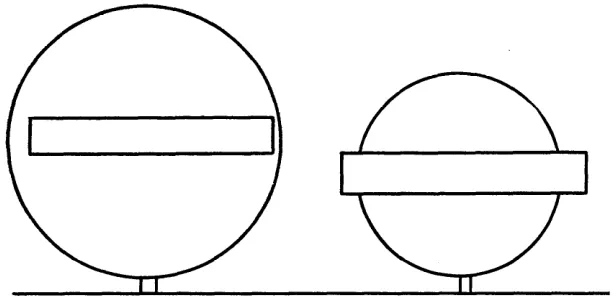
The variable-plot method re- quires no actual measurements in the field. No plots or lines are laid out on the ground, and it is un- necessary to measure the dimen- sions of any plant. The usual measured plots or lines are re- placed by a series of sampling points distributed at random throughout the area to be surveyed. At each sampling point, the observer views through the eyepiece of a hand-held angle gauge every shrub visible from that point. The angle gauge is illustrated in Fig- ure 1. Those shrubs are counted whose horizontal crown spread appears larger than the crossarm of the angle gauge. Shrubs whose crown spread appears less than the length of the crossarm are ignored. Figure 2 is a schematic diagram showing a shrub that would be counted and one that would not. The distance at which a shrub is

(2)

FIGURE 2. Schematic dkgram of two shrubs viewed with the angle gauge. The shrub on the left would be counted; the one on the right would not.

counted depends upon its size. Large shrubs are counted at a greater distance from the observer than small ones.

To determine shrub crown density in percent, it is necessary only to divide the average shrub count for all the sampling points by a s predetermined constant. This constant is determined by the dimen- sions of the angle gauge. The number of sampling points required on any area depends on the desired intensity of the survey.

Principle of the Methold The plots from which the method takes its name are entirely theoretical-they are not laid out on the ground. Each sampling point is the center .of several theoretical circular plots of varying radii

(Husch, 1956). At each sampling point, there are many overlapping plots with a common center, each plot corresponding to one of the shrubs counted with the angle gauge.

Let us assume that an angle gauge has an overall length of 30 inches, with a crossarm six inches long. When held to the eye, this gauge intercepts a horizontal angle of 9’25’. This angle just includes a circle at five times its diameter from the observer. A circle that intercepts a larger angle than 9 “25’ will appear larger than the instrument crossarm, and is closer to the eye than five times its diame: ter. One which intercepts a smaller

angle is farther away and will appear smaller than the cross arm. These relations follow from the fact that the overall length of the gauge is five times the length of its crossarm.

A small circle occupies one percent of the area of a large circle if the radius of the large circle is five times the diameter of the small one. For instance, a circle ten feet in diameter has an area of about 78.54 square feet. A large circle whose radius is five times the diameter of the small one, or fifty feet, has an area of 7,854 square feet. Thus, the small circle occupies one percent of the area of the large one.

Now let us consider a shrub stand as observed with the angle gauge from a single sampling point. Any shrub whose horizontal crown spread appears exactly equal to the length of the crossarm is five times its own diameter from the sampling point; if it appears to extend beyond the edges of the crossarm it is closer than this limit. These are the shrubs that are counted.

Each shrub counted with the angle gauge occupies one percent of the area of a hypothetical plot whose radius is five times the diameter of the shrub. When a shrub is observed with the angle gauge, a theoretical plot of this radius is automatically set up. The limits of this plot are established by the fact that if a shrub is outside the plot, it appears smaller than the

instrument crossarm and is not counted. Each shrub counted therefore represents one percent shrub cover, and the total number counted is the percent of shrub cover at that sampling point.

A numerical example may help make this clear. A shrub, exactly ten feet in diameter, is located 25 feet from a sampling point. When this plant is observed through the angle gauge, a theoretical plot fifty feet in radius is automatically set up, and the shrub is observed to lie within this plot. Since the area of the shrub is 78.54 square feet, and that of the plot is 7,854 square feet, the shrub occupies one percent of the theoretical plot. At first glance, it might appear that since this shrub is less than fifty feet from the plot center, it represents more than one percent ground cover. A little thought will show that this is not so. The angle gauge sets up a maximum limit beyond which shrubs are not counted, and any shrub within this limit represents one percent of the area of the hypothetical plot.

A second shrub ten feet in diameter forty feet from the observer is still within the fifty foot limit, and it also occupies one percent of the area of the plot. If these two are the only shrubs which lie within five times their own diameter from the plot center, the shrub density at that sampling point is two percent, no matter how many plants there may be on the area that are more than five times their diameter away. If, however, a shrub twenty feet in diameter is sixty feet from the observer, it also is less than five times its diameter away. Its theoretical plot has a radius of 100 feet, and the shrub occupies one percent of the plot. These three plants taken together then indicate a three percent ground cover at that sampling point.

(3)

VARIABLE PLOT METHOD FOR SHRUB DENSITY 113

this limit represents the percent of ground cover at that point. Many other shrubs will be visible from each sampling point, but only those that lie within the specified limit contribute to the estimate of ground cover. The variable-plot method is nothing more than a means of counting all the shrubs that lie within this limit.

The instrument just described is unwieldy and hard to use in the field. Better results are obtained if the crossarm is made smaller, thus intercepting a smaller angle. A smaller crossarm means that shrubs will be counted at a greater distance from the eye, and that more than one shrub will be need- ed to equal one percent ground cover. Therefore, with a smaller crossarm the shrub count must be divided by a constant to determine the percent of shrub density.

To determine the relation between this constant and the di- mensions of the instrument, it is necessary to consider the mathe- matics of the method. Percentage of ground cover may be written

n S2

P=- x 100 U-1

(2R) 2

where P is percentage, n is number of shrubs on the plot, S is shrub diameter in feet, and R is plot radius in feet. The angle gauge is so constructed that

W

S

-=-

₍₂₎

IJ

R

when W is the length of the crossarm and IJ is the overall length of the instrument (more precisely, the distance of the crossarm from the eye). Substituting in (l),

W2

P=nx- x 100 ₍₃₎

(2U2

This can be expressed in the form Il

w= ₍₄₎

n 5+---

P

If r is the constant by which the shrub count at any point must be divided to find the percentage of ground cover, then

Table 1. Convenient division factors and crossarm lengths. Division

Factor

1 2 3 4 5 6

Ratio of crossarm lengt,h to distance of crossarm from the eye

1:5 1: 7.07 1: 8.66 1:lO 1: 11.18 1: 12.27

Length of CPOSS- Width of cali- arm for instru- bration targkt at ment length of 100 feet from

30 inches the eye.

Inches Feet

6.0 20.00

4 15/64 14.14

3 E/32 11.54

3.0 10.00

2 11/16 8.94

2 29/64 8.15

P = -? and r = -? (5) P Substituting ;5) in equation (4)) the final form becomes

IA

w=- ₍₆₎

5Vr

It should be pointed out that this formula is mathematically not strictly accurate. A correction should be made for the fact that the line of sight intercepts a chord closer to the observer than the true crown diameter. The error due to omission of. this correction is so small as to be almost unde- tectable in variable-plot sampling. From equation (6) it can be seen that if an instrument is 30 inches long and has a division constant of 2, its crossarm must be 4.24 inches long. The ratio of crossarm length to the distance of the crossarm from the eye is 1:7.07. Table 1 lists several other convenient division constants, with their accompanying ratios and crossarm lengths.

Construction and Use of the

Instrument

The angle gauge can easily be made from a strip of hardwood and some scrap metal. Extruded aluminum angles of the “do-it- yourself” variety sold by hardware stores make excellent material for the eyepiece and crossarm. The angles should be about 11/4 inches on a side. The eyepiece should have a viewing hole about 3/s inch in diameter. An instrument length of about 30 inches is convenient. If it is much shorter, difficulty will be experienced in keeping both

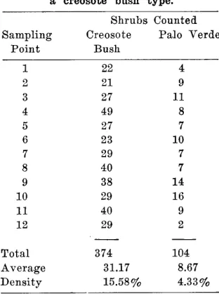
the crossarm and the more distant shrubs in focus at the same time. To illustrate the procedure fol- lowed in using the variable plot method, Table 2 lists the actual counts from a field trial made in an open stand of creosote bush (Larrecc triderztata) and palo Verde ( Cercidiwn

micro

pit

yllwrn)

.

The angle gauge was calibrated to require a division constant of 2. Twelve sampling points were located at arbitrary intervals of four chains, on two lines through the area. From each sampling point, those shrubs were counted whose diameters appeared larger than the crossarm. The counts were totaled and divided by 12 to find the average. This average was then divided by 2, the division constant of the instrument, to estimate the percentage of the area covered by shrubs. In this case, the total

Table 2. Sample variable-plot tally in a creosote bush type.

Shrubs Counted Sampling Creosote Pdo Verde

Point Bush

1 22 4

2 21 9

3 27 11

4 49 8

5 27 7

6 23 10

7 29 7

8 40 7

9 38 14

10 29 16

11 40 9

12 29 2

Total 374 104

Average 31.17 8.67

(4)

crown density of creosote bush was estimated at 15.6 percent; that of palo verde at 4.3 percent.

The principal difficulty in the use of the variable-plot method is that distant shrubs which should be counted tend to be obscured by those nearby. This difficulty is minimized by using a crossarm length which permits a division factor of 2. Shorter crossarms, with larger division constants, are occasionally useful in very sparse and open shrub stands. A longer crossarm, with a division constant of unity, becomes completely un- manageable, and introduces seri- ous errors.

In dense shrub stands, many distant shrubs are obscured and accuracy falls off rapidly. The method is not very reliable where densities exceed about 35 percent. For this reason, it is best suited to sparse desert-shrub types, to areas of shrub invasion in grasslands, and to other open types. Tf the plants are small, it is necessary to crouch down in order to keep the line of sight nearly horizontal.

Steep slopes require a correction of shrub counts to increase accur- acy. The count at any point is multiplied by the secant of the angle of slope perpendicular to the contour. An average slope correction can be used if shrub density does not change markedly with changes in slope.

Another possible source of trou- ble lies in the distance of the crossarm from the eye. It is this distance which determines the characteristics of the angle gauge, rather than the actual overall length of the instrument itself. It is best to use the following calibration procedure in adjusting the final position of the crossarm. Sup- port the instrument firmly and measure a distance of 100 feet from the eyepiece. At this distance, lay out a target at right angles to the line of sight. If the angle has a division constant of 2, the target should be 14.14 feet across. Sizes of target for other constants are listed in Table 1. With the eyepiece held firmly against the bones

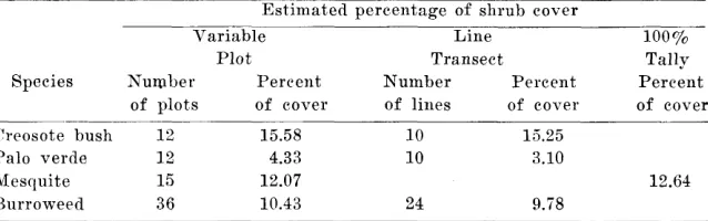
Table 3. Results of tests of variable-plot method in various shrub types. Estimated percentage of shrub cover

Variable Line 100%

Plot Transect Tally

Species Number Percent Number Percent Percent

of plots of cover of lines of cover of cover

Creosote bush 12 15.58 10 15.25

Palo Verde 12 4.33 10 3.10

Mesquite 15 12.07 12.64

Burroweed 36 10.43 24 9.i8

sllrrounding the eye, move the crossarm backward and forward on the wooden base until the target is exactly covered. Fasten the crossarm securely at this point. A slotted bolthole on the crossarm fa- cilitates calibration. If eyeglasses are worn, the instrument can be made shorter so that the eyepiece rests against the ,glasses.

The data obtained from variable-plot samples are subject to the usual statistical analyses. Com- monly used formulas can be used to compute standard deviation, standard error of the mean, and other useful statistics. Further- more, variable-plot data lend them- selves readily to the calculation of an index of dispersion. This index is a measure of the spatial distribu- tion of individual plants, indicat- ing whether they are more or less uniformly distributed than would be expected as a result of pure chance. Rice and Penfound (19%) describe in detail the method of calculating this illdex, whicll is of value in many ecological studies.

Bitterlich’s method was first used to measure basal area of tree stems in square feet per acre. For this purpose, a crossarm length to eye distance ratio of 1:33 has com- tionly been used, rather than the 1:7.07 recommended for shrubs. Estimates using this small crossarm have been found quite reliable in forest stands (Rice and Pen- found, 1955 ; Shanks, 1954). Husch

(1955) found that he obtained more accurate estimates of basal area by usin, “a a 1:16.5 ratio. All of these investigators found that the variable-plot method took much less time than the conventional methods with which it was compared.

Cumparisons with Other Sampling Methods

Several tests were made to com- pare the variable-plot procedure with standard estimating methods in diverse shrub types in southern Arizona. Results of these compari- sons are summarized in Table 3.

Data were available on the percentage of crown cover in a 6-acre stand of mesquite (Prosopsis jllli- florn). The crown area of each tree had previously been measured, and the percent of grqund cover determined. The complete tally showed a cover density of 12.64

percent, lvhile the variable-plot samples estimated density to be 12.07 percent.

The variable-plot method was next compared with the line transect method (Canfield, 1941) in common use by range technicians. As the line transect method is generally considered to give fairly reliable estimates of plant density, a comparison of the two methods will presumably give an index to the accuracy of the variable-plot technique.

The 12 variable-plot samples in the creosote bush stand previously described were compared with aLen 200-foot line transects run through the same area. The variable-plot samples gave a creosote bush density estimate of 15.58 percent, while the line transect estimate waq 15.25 percent. There was a greater difference in the palo *Verde estimates, which were 4.3 percent and 3.1 percent, respectively. How- ever, the palo verdes were so widely scattered that neither sample was adequate.

(5)

VARIABLE PLOT METHOD FOR SHRUB DENSITY 115

variable-plot samples was taken from the same sample points as in the first survey, using an instrument with a division constant of 4. Collection of the data for this second set of samples took longer than the first because of the greater number of shrubs that had to be counted, and to the greater effort required to avoid missing some. In spite of all precautions, a few were evidently missed, because the 4X angle gauge yielded a density estimate of only 14.3 percent for the creosote bush, compared with the previous estimate of 15.6 percent. The palo verde estimate was almost the same for the two instruments, because of the large size and small number of these trees, which were easily visible even at a distance.

A final comparison was made in a stand of burroweed (Happlopap- pus tenzhectus), a desert half- shrub averaging about one foot in diameter. Thirty-six variable-plot samples were compared with 24 line transects, each 100 ,feet long. The variable-plot density estimate was 10 43 percent, while that by

line transects was 9.7 percent. The difference between these two* results was less than the expected sampling error calculated for ei- ther method.

Since .lhese ‘tests compared one sampling method with another, it was not possible to calculate the statistical significance of the differ-

ence between them. IIowever, it has generally been considered that any sampling method is satisfac- tory that yields an estimate within 10 percent of the true cover density. The agreement between the variable-plot estimates and those made ,by other methods strongly suggests that density estimates made by the variable-plot method will fall well within these limits.

The variable-plot technique is most applicable where nearly circular objects are sampled. If shrub crowns are extremely irregular, considerable bias will be introduced. For this reason, the method is most useful in reconnaisance and extensive surveys. In forestry work, the angle prism suggested by Bruce (1955) has been widely adopted instead of a stick. This idea could be tried for estimating shrub cover, but the angle prism appears to have fewer advantages in counting ,shrubs than it does in counting small tree trunks.

Summary

The variable-plot method can be used to estimate shrub density in percent without measurement of distance or area. This method is faster and easier to apply than any of the standard shrub-estimating procedures now in common use. In tests in three different vegetation types, it closely approximated the

WALTER DUTTON, back from his

F.A.O. range assignment in Argentina, is enthusiastic about the future pos- siblilities for increased livestock produc- tion in that country. Breeding stand- ards are high. A fa,vora.ble climate over much of the area allows exceptionally long growing periods. Grazing capaci- ties on both natural grasslands and artificial pa.stures are outstanding-in many places 2 to 5 acres per hea.d per cow for one year. Currently, however, the outlook is not encouraging. Gen-

Report On Argentina

era1 failure during the growing period to convert surplus fora,ge to hay and silage for use in winter is the main stumbling block to increased produc- tion. All too common are low calving and lambing percentages, long periods for steels to reach maturity, and heavy incidence of f{?ot-and-mouth disease, stemlning directly from lack of adequate feed during critical periods. On the other hand, and indicative of what can be done, a few outfits are rnarket- ing 18 month old steers, weighing 1100

estimates obtained by other sam-

pling methods. It is most reliable in open shrub stands with a density of less than 35 percent ; beyond that point accuracy falls off rapidly. Variable-plot data are subject to statistical analysis, and are particularly useful in calculating an index of dispersion. The variable-plot method appears to be a practical means of reducing the labor required in collecting field data on &rub density.

LITERATURE CITED

BITTEIILI~H, W. 1948. Die Winkelzahl- probe. Allgcmcine Forst-und-Holzwirt- schaftliche Zeitung. 59 (l/a) : 4-5. BRUCE, DAVID. 1955. A new way to look

at trees. Jour. Forestry 53 : 163-167. CANFIELD, R. W. 1941. Application of

the line interception method in sampling range vegetation. Jour. Forestry :<9 : 388-394.

GKOSENHAUGII, L. R. 19.52. Plotless timber estimates-new, fast, easy. Jour. Forestry. 50: 32-37.

H~SCII, B. 19,X. Results of an inrestiga- tion of the variable plot method of cruising. Jour. Forestry. 53 : 570-574. -. 1956. Comments on the variable plot method of cruising. Jour. Forestry.

54: 41.

RICE, E. L. and W. T. PENFOUXD. 1955. An evaluation of the variable-radius and paired-tree methods in the black- jack-post oak forest. Ecology. 36: 335- 320.

SHANKS, R. E. 1954. Plotless sampling trials in Appalachian forest types. Ecology 35 : 237-244.

to 1200 pounds, from alfalfa-rye grass- hromegrass pastures without any sup- plemental feeding. In Patagonia, about 70 percent of the land is owned by the Federal Government but is entirely without any provision for management or protection such as that given Bu-